| Issue |
A&A
Volume 497, Number 3, April III 2009
|
|
|---|---|---|
| Page(s) | 889 - 910 | |
| Section | Celestial mechanics and astrometry | |
| DOI | https://doi.org/10.1051/0004-6361/20079054 | |
| Published online | 18 February 2009 | |
Tidal dynamics of extended bodies in planetary systems and multiple stars
S. Mathis1,2 - C. Le Poncin-Lafitte3
1 - Laboratoire AIM, CEA/DSM - CNRS - Université Paris Diderot, IRFU/Service d'Astrophysique, CEA-Saclay, 91191 Gif-sur-Yvette Cedex, France
2 -
LUTH, Observatoire de Paris - CNRS - Université Paris-Diderot; Place Jules Janssen, 92195 Meudon Cedex, France
3 -
SYRTE UMR8630, Observatoire de Paris, 61 avenue de l'Observatoire, 75014 Paris, France
Received 12 November 2007 / Accepted 8 December 2008
Abstract
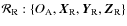
Context. With the discovery during the past decade of a large number of extrasolar planets orbiting their parent stars at distances lower than 0.1 astronomical unit (and the launch and the preparation of dedicated space missions such as CoRoT and KEPLER), with the position of inner natural satellites around giant planets in our Solar System and with the existence of very close but separated binary stars, tidal interaction has to be studied carefully.
Aims. This interaction is usually studied with a punctual approximation for the tidal perturber. The purpose of this paper is to examine the step beyond this traditional approach by considering the tidal perturber as an extended body. To achieve this, we studied the gravitational interaction between two extended bodies and, more precisely, the interaction between mass multipole moments of their gravitational fields and the associated tidal phenomena.
Methods. We use cartesian symmetric trace free tensors, their relation with spherical harmonics and Kaula's transform enables us to analytically derive the tidal and mutual interaction potentials, as well as the associated disturbing functions in extended body systems.
Results. The tidal and mutual interaction potentials of two extended bodies are derived. In addition, the external gravitational potential of such a tidally disturbed extended body is obtained, using the Love number theory, as well as the associated disturbing function. Finally, the dynamical evolution equations for such a system are given in their more general form without any linearization. We also compare, under a simplified assumption, this formalism to the punctual case. We show that the non-punctual terms have to be taken into account for strongly deformed perturbers (
 )
in very close systems (
)
in very close systems (
 ).
).
Conclusions. We show how to derive the dynamical equations for the gravitational and tidal interactions between extended bodies and associated dynamics. The conditions for applying this formalism are given.
Key words: gravitation - celestial mechanics
1 Introduction
In celestial mechanics, one of the main approximations done in the modeling of tidal effects (star-star, star-innermost planet or planet-natural satellites interactions) is to consider the tidal perturber as a point-mass body. However a large number of extrasolar Jupiter-like planets orbiting their parent stars at a distance less than 0.1 AU have been discovered during the past decade (Mayor et al. 2005). Moreover, in Solar System, Phobos around Mars and the inner natural satellites of Jupiter, Saturn, Uranus, and Neptune are very close to their parent planets. In such cases, the ratio of the perturber mean radius to the distance between the center of mass of the bodies cannot be any more negligible compared to 1 (cf. Fig. 1). Furthermore, it can also be the case for very close, but separated, binary stars. In that situation, neglecting the extended character of the perturber has to be relaxed, so the tidal interaction between two extended bodies must be solved in a self-consistent way by taking the full gravitational potential of the extended perturber into account, generally expressed with some mass multipole moments, and then to consider their interaction with the tidally perturbed body. In the literature, not many studies have been done (Borderies 1978, 1980; Ilk 1983; Borderies & Yoder 1990; Hartmann et al. 1994; Maciejewski 1995). The purpose of this work is then to provide a theoretical procedure for obtaining this tidal gravitational interaction, as well as its associated tidal dynamical evolution.Several years ago, Hartmann et al. (1994) introduced an interesting tool in celestial mechanics, based on cartesian symmetric trace free (STF) tensors, to treat the couplings straighforwardly between the gravitational fields of extended bodies. These tensors are fully equivalent to the usual spherical harmonics, but in addition, a set of STF tensors represents an irreductible basis of the rotation group SO3 (Courant & Hilbert 1953; Gelfand et al. 1963). It means that, by using algebraic properties of STF tensors with the index notation of Blanchet & Damour (1986), these objects become a powerful tool for determining the coupling between spherical harmonics in an elegant and compact way. However, as these tensors are not widely used in celestial mechanics, we first recall their definition and fundamental properties and stress their relation to the usual spherical harmonics. Then, we treat the multipole expansion of gravitational-type fields for which each type is related to a given extended body. First, the well-known external field of such body is derived using STF tensors; classical identities are provided. Next, the mutual gravitational interaction between two extended bodies and the associated tidal interaction are derived. We show how the use of STF tensors leads to an analytical and compact treatment of the coupling of their gravitational fields. We deduce the general expressions of tidal and mutual interaction potentials expanded in spherical harmonics. Using classical Kaula's transform (Kaula 1962), we express them as a function of the Keplerian orbital elements of the body considered as the tidal perturber. These results are used to derive the external gravitational potential of such tidally perturbed extended body. After introducing a third body, its mutual interaction potential with the previous tidally perturbed extended body is defined that allows us to derive the disturbing function using the results obtained with STF tensors and Kaula's transform. At this stage, the different type of mutual gravitational interaction is defined. The dynamical equations ruling the evolution of this system are obtained. Finally, we use a reduced form of that equations to qualitatively quantify the influence of non-punctual terms of the disturbing function in comparison with the punctual case.
![\begin{figure}
\par\includegraphics[width=12cm,clip]{9054fig1.eps}
\end{figure}](/articles/aa/full_html/2009/15/aa9054-07/img39.png) |
Figure 1:
System of two extended bodies.
|
| Open with DEXTER | |
 and
and
 are the respective mean radius of A and B, while
 is the distance between their respective center of mass.
 are the conical angles with which each perturber is seen from the center of mass of the perturbed body. When
 with i=A or B, the ith body could be considered as a punctual mass perturber.
2 STF-Multipole expansion of gravitational potentials
2.1 Definitions and notations
We focus first on the STF tensors. Let us define a Cartesian l-tensor as a set of numbers
Ti1i2...il with l different indices i1 to il, each taking an integer value running between 1 and 3. A compact multi-index notation, first introduced by Blanchet & Damour (1986), is generally used. An uppercase Latin letter denotes a multi-index, while the corresponding lowercase denotes its number of indices:
| (1) |
The Einstein summation convention is assumed in the following, so if some index appears twice, a summation over that index is implied
 |
(2) |
Given a Cartesian tensor
 ,
we denote its symmetric part with parenthesis
,
we denote its symmetric part with parenthesis
where
 runs over all the l! permutations of
 .
.
Next, the symmetric trace tree part of a tensor
is denoted indifferently by
![]() .
Following Thorne (1980), the STF part of
reads as
.
Following Thorne (1980), the STF part of
reads as
where
 is the classical Kronecker delta function,
 |
(5) |
 denoting the integer part of
 while
while
2.2 STF-basis
Let  (i running between 1 and 3) be a Cartesian basis vectors set (with the rule
 ). The basis of the (2l+1)-dimensional vector space of STF rank l-tensors is made of the STF parts of the l-fold tensorial products (Thorne 1980)
 |
(6) |
where
 |
(7) |
with i2=-1. For m>0, let us define the following algebraic object
 |
(8) |
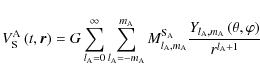
Then, the STF canonical basis is proportional to
 and can be chosen as (Thorne 1980):

where
The constant Alm is chosen to get a normalization, such that
z* corresponding to the complex conjugate of z, z being a complex number or function. Finally, taking Eqs. (4), (9), and (10) into account, we obtain
where
 |
(13) |
Let us consider an arbitrary vector
 .
We can now introduce the Euclidean norm r of
.
We can now introduce the Euclidean norm r of  ,
the corresponding unit vector
,
the corresponding unit vector  and the Cartesian tensors xK and nK constructed on
as
and the Cartesian tensors xK and nK constructed on
as
Using the harmonic property
 (for r>0) and Eq. (14), one gets
where
 and
and  are the STF part of
 and nL, respectively. Then, considering Eq. (12) and taking
into account, the computation of Kronecker deltas functions combined with Eq. (15) leads to
and nL, respectively. Then, considering Eq. (12) and taking
into account, the computation of Kronecker deltas functions combined with Eq. (15) leads to

By applying Eq. (16) twice, we find
![$\displaystyle \hat{\cal Y}^{l,m}_L\hat{\partial}_L\left[\hat{\cal Y}^{j,k}_J\hat{\partial}_J\left(\frac{1}{r}\right)\right]$](/articles/aa/full_html/2009/15/aa9054-07/img76.png) |
= |  |
|
| = |  |
(17) |
This last equation leads to a composition law of a product of basis functions
 .
After some algebra, we obtain
.
After some algebra, we obtain
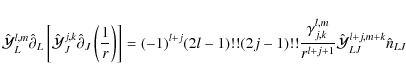
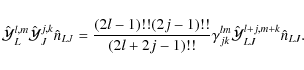
where
![\begin{displaymath}\gamma_{jk}^{lm}=\gamma_{lm}^{jk}=\sqrt{\frac{2l+1}{(l+m)!(l-...
...+k\right)\right]!}{4\pi\left[2\left(l+j\right)+1\right]}}\cdot
\end{displaymath}](/articles/aa/full_html/2009/15/aa9054-07/img81.png) |
(19) |
Considering that the lefthand side of the Eq. (18) can be written using Eq. (15) as
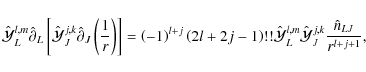 |
(20) |
we finally get
2.3 Relation between STF-basis and usual spherical harmonics
In this section the equivalence between STF basis and spherical harmonics Yl,m is given. Following Abramowitz & Stegun (1970), Yl,m reads as

![$\displaystyle {\mathcal N_{lm}}\left(\exp\left[{\rm i}\varphi\right]\sin\theta\...
...um_{j=0}^{\left\lbrack\frac{l-m}{2}\right\rbrack}a^{lmj}(\cos\theta)^{l-m-2j} ,$](/articles/aa/full_html/2009/15/aa9054-07/img86.png)
where the Plm are the classical associated Legendre polynomials. We also recall the symmetry property of the Yl,m, namely,

Since the components of the unit vector
in complex form is
![\begin{displaymath}
n_x+{\rm i}n_y=\exp\left[{\rm i}\varphi\right]\sin\theta , \quad n_z=\cos\theta ,
\end{displaymath}](/articles/aa/full_html/2009/15/aa9054-07/img88.png)
we can identify
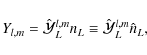
which can be inverted by using Eq. (11) as
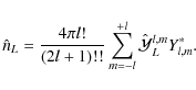
To give an example of how it works, let us examine the cases l=0 and l=1. The spherical harmonics are
 |
(27) |
![\begin{displaymath}Y_{1,0}=\sqrt{\frac{3}{4\pi}}\cos\theta~ , \quad Y_{1,1}=-\sqrt{\frac{3}{8\pi}}\sin\theta \exp\left[{\rm i}\varphi\right] .
\end{displaymath}](/articles/aa/full_html/2009/15/aa9054-07/img92.png) |
(28) |
Let us compare with the STF-basis functions. For l=0, the normalization rule given in Eq. (11) gives the single number
 .
For l=1 we have
.
For l=1 we have
 |
(29) |
so it is verified that
 .
.
2.4 Multipole expansion of the external gravitational field of an extended body
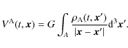
Let us consider some matter distribution, corresponding to a body A, in the inertial coordinates (t,xi). The Newtonian gravitational potential of this body,
 ,
is obtained by solving the Poisson equation
,
is obtained by solving the Poisson equation
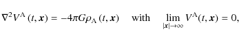 |
(30) |
with
 its density. This leads to an expression of
 ,
where
,
where  is the equatorial radius of A, to
 |
(31) |
Then, the external gravitational field of the body A for
 can be represented by the series:
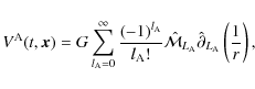
where all mass multipole moments are defined by

and the usual gravitational moments in the physical space are given by
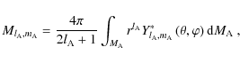
where
 is the mass of A and
 for
is thus obtained:
for
is thus obtained:
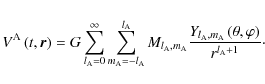
One should note the symmetry property of
 :
:
Moreover,
can be represented in its polar form
![\begin{displaymath}M_{l_{\rm A},m_{\rm A}}=\vert M_{l_{\rm A},m_{\rm A}}\vert\exp\left[{\rm i}\delta M_{l_{\rm A},m_{\rm A}}\right],
\end{displaymath}](/articles/aa/full_html/2009/15/aa9054-07/img111.png) |
(37) |
where the following identities are obtained from Eq. (36)
 |
(38) |
Using the classical symmetry property concerning spherical harmonics given in Eq. (23),
 could also be expressed with the associated Legendre polynomials:
![\begin{displaymath}V^{\rm A}\left(t,\vec r\right)=G\sum_{l_{\rm A}=0}^{\infty}\s...
...{l_{\rm A},m_{\rm A}}\sin\left(m_{\rm A}\varphi\right)\right],
\end{displaymath}](/articles/aa/full_html/2009/15/aa9054-07/img114.png) |
(39) |
where the usual coefficients
 and
and
 are given by
 |
(40) |
The expression of
and
 are then deduced for
 :
:
 |
(41) |
![\begin{displaymath}\delta M_{l_{\rm A},m_{\rm A}}=-{\rm Arctan}\left[\frac{\left...
...{S_{l_{\rm A},m_{\rm A}}}{C_{l_{\rm A},m_{\rm A}}}\right]\cdot
\end{displaymath}](/articles/aa/full_html/2009/15/aa9054-07/img121.png) |
(42) |
In the general case, the gravitational moments are expanded as
Both
 and
and
 are respectively those in the case where A is isolated (without any perturber) and those induced by the tidal perturber(s).
One can identify some special values of
relevant to the gravitational field of a body A. The trivial one is its mass,
 |
(44) |
Furthermore, we know that the external field of an axisymmetric body A can be expressed as a function of the usual multipole moment

![\begin{displaymath}V^{\rm A}\left(t,\vec r\right)=\frac{GM_{\rm A}}{r}\left[1-\s...
...right)^{l_{\rm A}}P_{l_{\rm A}}\left(\cos\theta\right)\right];
\end{displaymath}](/articles/aa/full_html/2009/15/aa9054-07/img127.png) |
(45) |
using Eq. (35), we identify in a straigthforward way:
 |
(46) |
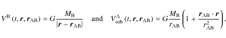
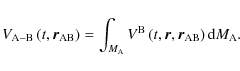
We can now focus on the second type of gravitational interaction, namely the tides between two extended bodies.
2.5 Determination of the tidal potential
Let us now introduce an accelerated reference frame, i.e.
 ,
associated with a body A, which is related to a global inertial frame through the transformation
,
associated with a body A, which is related to a global inertial frame through the transformation
 |
(47) |
 being the arbitrary motion of the local A-frame. The equations of motion with respect to the local A-frame reads (Damour et al. 1993):
where
 being the velocity with respect to this frame, while tij denotes the stress tensor. The following effective potential appears as
where
 |
(51) |
the considered body A being tidally interacting with N-1 perturbing extended bodies B;
 is the potential of each body B different from A.
The last term of Eq. (50) represents the inertial effects on the accelerated local frame A. This effective potential can be split into the potential of A given in Eq. (35) and a tidal potential,
is the potential of each body B different from A.
The last term of Eq. (50) represents the inertial effects on the accelerated local frame A. This effective potential can be split into the potential of A given in Eq. (35) and a tidal potential,
 ,
as
,
as
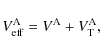 |
(52) |
the tidal part being given by
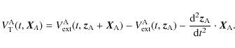 |
(53) |
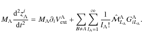
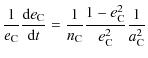
By integrating the equations of motion Eqs. (48) and (49) over the body A, we get the equations for the conservation of the total mass of A,
 ,
and for the second time derivative of the local dipole moment
,
and for the second time derivative of the local dipole moment
 (Damour et al. 1992; Hartmann et al. 1994):
 |
(54) |
We can now derive the expression of
into series by using an STF expansion of ascending powers of
 as
as
 |
(56) |
where
 are the local effective tidal moments with
We assume that the origin of the local A-frame coincides with the center of mass of A; i.e., the dipole moment
 vanishes. Since now the
 indices are related to their associated body: for example, for A we use
 while for B we use
 .
With these definitions, the righthand side of Eq. (55) can be written as
.
With these definitions, the righthand side of Eq. (55) can be written as
The local equation of motion is finally obtained from the d'Alembert principle with
 |
(60) |
which leads, by using Eqs. (59) and (57), to
 |
(61) |
Expressing
in terms of Eq. (32) as in Hartmann et al. (1994), we finally obtain
Using Eqs. (57), (58) and (62), the tidal potential can be expressed as
Using Eq. (15), we get
that leads, taking into account Eq. (33), to

We now replace the Cartesian multipole moments by their spherical harmonics representation. First of all, using Eq. (26) and putting
 |
(66) |
 |
(67) |
Then, the last term of Eq. (65) involving the product of basis function
 can be written by using Eq. (21) as follow
Noting that the STF derivative in the RHS of Eq. (68) can be split into two parts,
 |
(69) |
and using the relation given by Hartmann et al. (1994)
we get
Inserting Eqs. (68) and (71) into Eq. (65), using Eq. (25) with

The respective physical meanings of terms I and
 are clearly identified. Term I corresponds to the gravitational interaction of B with A, while term
is the acceleration responsible for the movement of the center of mass of A. In the case of a punctual mass perturber B, we recall that we get (see for example Melchior 1971)
are clearly identified. Term I corresponds to the gravitational interaction of B with A, while term
is the acceleration responsible for the movement of the center of mass of A. In the case of a punctual mass perturber B, we recall that we get (see for example Melchior 1971)
 |
(73) |
where
 |
(74) |
with
 its mass.
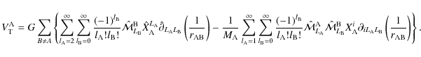
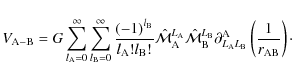
Equation (72) exactly corresponds to the Eq. (3.25) given in Hartmann et al.
(1994) that we recall here:
 |
= | 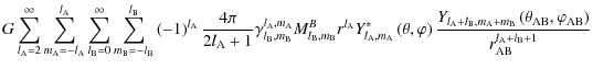 |
|
![$\displaystyle -\frac{G}{M_{\rm A}}\sum_{l_{\rm A}=1}^{\infty}\sum_{m_{\rm A}=-l...
...a_{\rm AB},\varphi_{\rm AB}\right)}{r_{\rm AB}^{l_{\rm A}+l_{\rm B}+1}}\right].$](/articles/aa/full_html/2009/15/aa9054-07/img184.png) |
(75) |
It is then recast in its general spectral form, using that
is real and expanding it in the spherical harmonics for
,
where the coefficients
 and
and
 are respectively given by
and

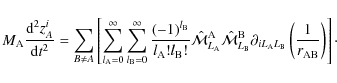
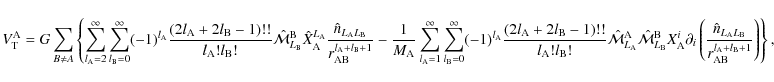
Once the more general form of the tidal potential is derived, we now express
and
as a function of the Keplerian orbit elements of the perturber B.
Here, we take into account the relative inclinations of the spin of each body with respect to the orbital plane. It is then necessary to define three reference frames, represented in Fig. 3, all centered on the center of mass of the considered body A,  :
:
- An inertial frame
 :
:
 ,
time independent, with
,
time independent, with
 in the direction of the total angular momentum of the whole system
 which is a first integral. (We are studying here the two bodies interaction between A and each potential perturber
 with
with
![$k\in\left[\!\left[1,N\right]\!\right]$](/articles/aa/full_html/2009/15/aa9054-07/img198.png) .)
.)
- An orbital frame
 :
:
 .
We define here three Euler angles to link this frame to
:
:
.
We define here three Euler angles to link this frame to
:
:
 ,
the inclination of the orbital frame with respect to
,
the inclination of the orbital frame with respect to
 ;
;
-
 ,
the argument of the pericenter;
,
the argument of the pericenter;
-
 ,
the longitude of the ascending node.
,
the longitude of the ascending node.
 ,
the semi major axis,
,
the semi major axis,  ,
the eccentricity, and
,
the eccentricity, and
 ,
the mean anomaly with
,
the mean anomaly with
 ,
where
,
where  is the mean motion.
- A spin equatorial frame
 :
:
 .
This frame is rotating with the angular velocity,
.
This frame is rotating with the angular velocity,
 .
This frame is linked to
.
This frame is linked to
 by three Euler angles:
-
 ,
the obliquity, i.e. the inclination of the equatorial plane with respect to the reference plane
;
,
the obliquity, i.e. the inclination of the equatorial plane with respect to the reference plane
;
-
 ,
the mean sideral angle where
,
the mean sideral angle where
 .
This is the angle between the minimal axis of inertia and the straight line due to the intersection of the planes
.
This is the angle between the minimal axis of inertia and the straight line due to the intersection of the planes
 and
.
and
.
-
 ,
the general precession angle.
,
the general precession angle.
-
![\begin{displaymath}\frac{Y_{l,m}\left(\theta_{\rm AB},\varphi_{\rm AB}\right)}{r...
...left(e_{\rm B}\right)\exp\left[{\rm i}\Psi_{l,m,j,p,q}\right],
\end{displaymath}](/articles/aa/full_html/2009/15/aa9054-07/img218.png)
where the
 coefficients are given by
Here
 is the obliquity function which is defined as follow for
  :
:
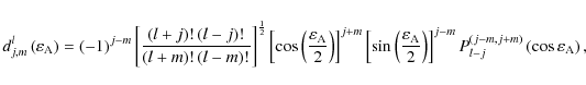
the
 being the Jacobi polynomials (cf. Abramowitz & Stegun 1972). The value of the function for indices j, which do not verify
are deduced from
being the Jacobi polynomials (cf. Abramowitz & Stegun 1972). The value of the function for indices j, which do not verify
are deduced from
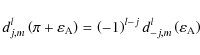 |
(82) |
or from their symmetry properties:
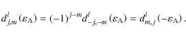 |
(83) |
On the other hand, one should note that
 .
.
![\begin{figure}
\par\includegraphics[width=12cm,clip]{9054fig2.eps}
\end{figure}](/articles/aa/full_html/2009/15/aa9054-07/img230.png) |
Figure 2:
Spherical coordinate system associated to the equatorial reference frame
|
| Open with DEXTER | |
 :
:
 of an extended body A; we have
 and
and
 ,
,
 and
and
 are the coordinates of the center of mass of the potential extended perturber B.
![\begin{figure}
\par\includegraphics[width=12cm,clip]{9054fig3.eps}
\end{figure}](/articles/aa/full_html/2009/15/aa9054-07/img232.png) |
Figure 3:
Inertial reference, orbital, and equatorial rotating frames (
|
| Open with DEXTER | |
 )
and associated Euler's angles of orientation.
)
and associated Euler's angles of orientation.Table 1:
Values of the obliquity function
 in the case where l=2 and
obtained from Eq. (81) (adapted from Yoder 1995).
in the case where l=2 and
obtained from Eq. (81) (adapted from Yoder 1995).
The inclination function,
 ,
is defined in a similar way:
,
is defined in a similar way:
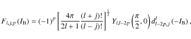 |
(84) |
where
![\begin{displaymath}Y_{l,m}\left(\frac{\pi}{2},0\right)=\left[\frac{2l+1}{4\pi}\r...
...ght)/2\right]!}\cos\left[\left(l-m\right)\frac{\pi}{2}\right];
\end{displaymath}](/articles/aa/full_html/2009/15/aa9054-07/img242.png) |
(85) |
moreover, the following symmetry property is verified:
![\begin{displaymath}F_{l,-j,p}\left(I_{\rm B}\right)=\left[\left(-1\right)^{l-j}\...
...t)!}{\left(l+j\right)!}\right]F_{l,j,p}\left(I_{\rm B}\right).
\end{displaymath}](/articles/aa/full_html/2009/15/aa9054-07/img243.png)
The usual value of these functions are given in Table 2.
Table 2:
Values of the inclination function
 in the case where l=2, and values for j<0 can be deduced from Eq. (86) (adapted from Lambeck 1980).
The eccentricity functions
 ,
are polynomial functions having
,
are polynomial functions having
 for argument (see Kaula 1962; and Laskar 2005, for their detailed properties). Their values for the usual sets
 are given in the Table 3. In the case of weakly eccentric orbits, the summation over a small number of values for q is sufficient (
![$q\in\left[\!\left[-2,2\right]\!\right]$](/articles/aa/full_html/2009/15/aa9054-07/img254.png) ). More details can be found in the appendix of Yoder (1995).
). More details can be found in the appendix of Yoder (1995).
Table 3:
Values of the eccentricity function
 in the case where l=2 (adapted from Lambeck 1980), where several combinations
have the same Gl,p,q value.
in the case where l=2 (adapted from Lambeck 1980), where several combinations
have the same Gl,p,q value.
Finally, the phase argument is given by
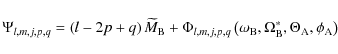
where
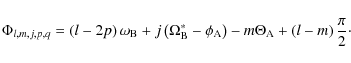 |
(88) |
This can be also written as
 |
(89) |
where we have defined the tidal frequency:
and
 |
(91) |
Kaula's transform allows us to express each function of
 ,
i.e. of
,
i.e. of
 ,
as a function of the Keplerian relative orbital elements of B in the A-frame. Applying Eq. (79) to
and
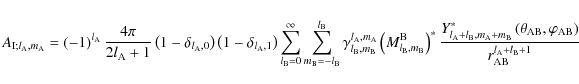
respectively given in Eqs. (77) and (78), we get
,
as a function of the Keplerian relative orbital elements of B in the A-frame. Applying Eq. (79) to
and
respectively given in Eqs. (77) and (78), we get

![$\displaystyle \left(-1\right)^{l_{\rm A}}\frac{4\pi}{2l_{\rm A}+1}\left(1-\delt...
...B}}^{\rm B}\vert\exp\left[-{\rm i}\delta M_{l_{\rm B},m_{\rm B}}^{\rm B}\right]$](/articles/aa/full_html/2009/15/aa9054-07/img270.png)
![$\displaystyle \times\frac{1}{a_{\rm B}^{l_{\rm A}+l_{\rm B}+1}}\sum_{j=-\left(l...
...) \exp\left[-{\rm i}\Psi_{l_{\rm A}+l_{\rm B},m_{\rm A}+m_{\rm B},j,p,q}\right]$](/articles/aa/full_html/2009/15/aa9054-07/img271.png)
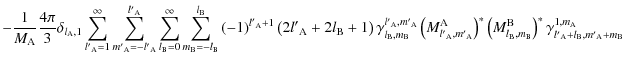
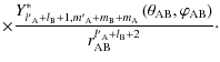
and
![$\displaystyle -\frac{1}{M_{\rm A}}\frac{4\pi}{3}\delta_{l_{\rm A},1}\sum_{l{'}_...
...B}}^{\rm B}\vert\exp\left[-{\rm i}\delta M_{l_{\rm B},m_{\rm B}}^{\rm B}\right]$](/articles/aa/full_html/2009/15/aa9054-07/img272.png)
whereas in Eq. (43)
Like in Zahn (1966a, 1977), the tidal potential can be split into two components. The first one,
 ,
is stationary (i.e. the tidal frequency vanishes:
,
is stationary (i.e. the tidal frequency vanishes:  ). It corresponds to the axisymmetric permanent deformation induced by B. In the case of a punctual mass perturber and of a system where all the spins are aligned, Zahn (1966a, 1977) showed that
![]() .
Then, the second component is the time-dependent part of the perturbation,
.
Then, the second component is the time-dependent part of the perturbation,
 ,
for which
,
for which
 .
.
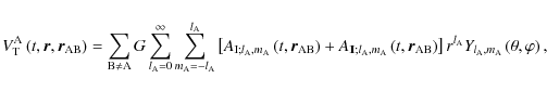
2.6 The two-body interaction potential
The mutual gravitational interaction potential![]() of two bodies A and B is defined as
of two bodies A and B is defined as
 |
(94) |
Following Hartmann et al. (1994), its expansion on STF-tensors is given by
 |
(95) |
Using once again Eqs. (18) and (33), we get
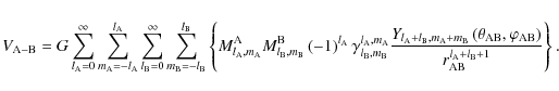
Finally, using Kaula transformation given in Eqs. (79), (80), and (87) as previously done for
,
 is expressed as a function of the obliquity,
,
and of the Keplerian orbital elements of B: ,
and :
is expressed as a function of the obliquity,
,
and of the Keplerian orbital elements of B: ,
and :
 |
= |  |
|
![$\displaystyle \times{ \frac{1}{a_{\rm B}^{l_{\rm A}+l_{\rm B}+1}}\sum_{v=-\left...
...eft[{\rm i}\Psi_{l_{\rm A}+l_{\rm B},m_{\rm A}+m_{\rm B},v,w,b}\right]\Bigg\}}.$](/articles/aa/full_html/2009/15/aa9054-07/img289.png) |
(97) |
This interaction potential contains all multipole-multipole couplings. It is used in Sect. 3.2 to compute the disturbing function aimed at studying the dynamics of an extended body in gravitational interaction with A.
Since all types of gravitational potentials have been examined, we now study the dynamics of a system of extended bodies.
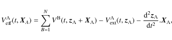
3 Equations of motion
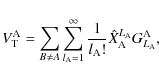
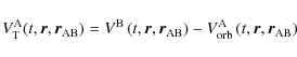
3.1 External gravitational potential of a tidally perturbed body
The goal of this section is to derive the external gravitational potential of a tidally perturbed extended body A by an extended body B. This potential is the sum of the structural self-gravitational potential of A,
 ,
and of
,
and of
 ,
the tidally induced gravitational potential corresponding to the response of A to the perturbing potential
,
the tidally induced gravitational potential corresponding to the response of A to the perturbing potential
 ,
,
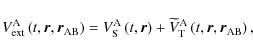 |
(98) |
with the following definition for
 :
:
 |
(99) |
where
are the multipole moments of A in the case where it is not tidally perturbed by any other body, in other words, in the case it is isolated. By definition the external gravitational potential is harmonic; therefore
 verifies the Laplace equation,
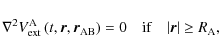 |
(100) |
that directly leads to the same equation for
:
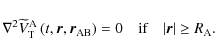 |
(101) |
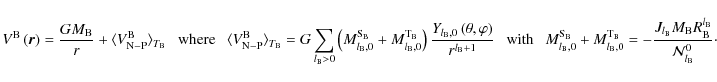
Following Lambeck (1980), Néron de Surgy (1996), Néron de Surgy & Laskar (1997), and Correia & Laskar (2003,b), we use the classical Love numbers,
 ,
which allow us to characterize the response of the body A to the tidal perturbation. The boundary conditions for
are
,
which allow us to characterize the response of the body A to the tidal perturbation. The boundary conditions for
are
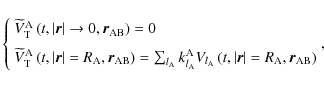
where
 is the
 spherical harmonic of
.
We also recall that when using Eq. (76)
has been expanded as follow for
:
spherical harmonic of
.
We also recall that when using Eq. (76)
has been expanded as follow for
:
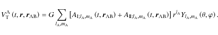
Using the well-known properties of the Laplace's equation, we search the solution for
 when
when
 of the form
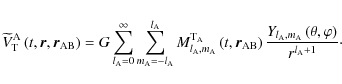
Inserting Eqs. (103) and (104) into (102), the final solution of
is then derived with

where
 and
and
 are given by
The response of body A, which is described by the Love numbers, is the adiabatic one. However, it is well known that both elastic and fluid bodies react to the tidal perturbation with a damping and a time delay that are caused by the internal friction and diffusivities (in other words, to the viscosity,
 ,
and the thermal diffusivity, K, in a non-magnetic body). That allows us to transform the mechanical energy into a thermal one, which leads us to the dynamical evolution of the studied system (cf. Fig. 4). We, therefore, introduce a complex impedance,
,
and the thermal diffusivity, K, in a non-magnetic body). That allows us to transform the mechanical energy into a thermal one, which leads us to the dynamical evolution of the studied system (cf. Fig. 4). We, therefore, introduce a complex impedance,
 ,
with its associated argument,
,
with its associated argument,
 ,
,
![\begin{displaymath}Z_{{\rm T}_{\rm A}}\left(\nu,K;\Psi_{L}\right)=\vert Z_{{\rm ...
... i} \delta_{{\rm T}_{\rm A}}\left(\nu,K;\Psi_{L}\right)\right]
\end{displaymath}](/articles/aa/full_html/2009/15/aa9054-07/img314.png) |
(107) |
which describes this damping. We thus substitute
in Eq. (106). Here, L corresponds to the indices of the considered tidal Fourier's mode and
and
 are described in Alexander (1973), Zahn (1977), and Correia & Laskar (2003).
![\begin{figure}
\par\includegraphics[width=12cm,clip]{9054fig4.eps}
\end{figure}](/articles/aa/full_html/2009/15/aa9054-07/img317.png) |
Figure 4:
Classical tidal dynamical system. The extended body B is tidally disturbing the extended body A, which adjusts with a phase lag
|
| Open with DEXTER | |
 are respectively the spin frequency of A and the respective mean motions of B and C.
Using Eqs. (92) and (93), the expressions of
and
are obtained:


where
As for
,
can be split into two components. The first one
 is stationary. It corresponds to the permanent component
 for which the tidal frequency ()
vanishes. The second component
for which the tidal frequency ()
vanishes. The second component
 is the time-dependent one that corresponds to
 for which
.
for which
.
Finally the external potential of A is thus written in its more compact and general form for
:
 |
(110) |
where

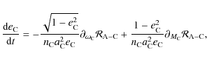
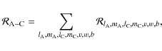
3.2 Disturbing function
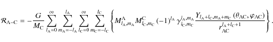
The goal of this section is to derive the disturbing function,
 ,
due to a tidally perturbed body A, acting on a body C for which the dynamics are studied and which can be different from the perturber body B (see Fig. 4).
,
due to a tidally perturbed body A, acting on a body C for which the dynamics are studied and which can be different from the perturber body B (see Fig. 4).
First, the disturbing function is related to the mutual gravitational interaction potential (cf. Tisserand 1889, 1891; Correia 2001) through
 |
(112) |
the sign being due to the potentials convention adopted here.
Using the definition of
 given in Eq. (96), we deduce the explicit spectral expansion of
 in the spherical harmonics:
 |
(113) |
The
 ,
,
 are respectively the mass multipole moments of the body A and of the body C, while
 ,
,
 ,
and
,
and
 are the spherical coordinates of the center of mass of the body C in the A-frame (cf. Fig. 2). Then, using Kaula's transform given in Eqs. (79), (80), and (87),
is expressed as a function of the obliquity,
,
and of the Keplerian orbital elements of C:
are the spherical coordinates of the center of mass of the body C in the A-frame (cf. Fig. 2). Then, using Kaula's transform given in Eqs. (79), (80), and (87),
is expressed as a function of the obliquity,
,
and of the Keplerian orbital elements of C:  ,
,
 and
and  :
:

![$\displaystyle \times{ \frac{1}{a_{\rm C}^{l_{\rm A}+l_{\rm C}+1}}\sum_{v=-\left...
...eft[{\rm i}\Psi_{l_{\rm A}+l_{\rm C},m_{\rm A}+m_{\rm C},v,w,b}\right]\Bigg\}}.$](/articles/aa/full_html/2009/15/aa9054-07/img344.png)
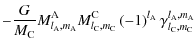
Here, three types of gravitational interaction are treated in our formalism (see also Eq. (111)). To describe them, one has first to consider the two causes of the multipolar behavior of the gravitational potential of a body. The first is due to its internal structure and dynamics. In the case of a solid body, it is due to its proper asymmetry, while in the case of a fluid mass, the internal dynamical processes such as rotation or magnetic field will break the ideal spherical hydrostatic symmetry of the body. The second is the deformation of the body due to its response to the tidal perturbation exerted by the perturber(s). In the case studied here, it is the response of the body A to the perturbation exerted by B computed in the previous section. Therefore, we split here the k-indexed mass multipole moments of each body as in Eq. (43):
where
 is the self-structural contribution of the body, while
 is the tidal one.
The three types of gravitational interaction are thus identified. The first is the interaction between the structural mass multipole moments of each body,
 with
with
 ;
one should note that
;
one should note that
 -
-
 is the classical interaction between
and
is the classical interaction between
and  ,
being the mass of C. The second corresponds to the mixed interaction between the structural and the tidal mass multipole moments,
,
being the mass of C. The second corresponds to the mixed interaction between the structural and the tidal mass multipole moments,
 .
The third is the interaction between the tidal mass multipole moments of each body,
.
The third is the interaction between the tidal mass multipole moments of each body,
 .
Therefore, the disturbing function could be split into three terms:
.
Therefore, the disturbing function could be split into three terms:
| (116) |
where
 is the disturbing function associated to the structure-structure interaction,
 is associated to the tide-structure interaction and
 is associated to the tide-tide interaction.
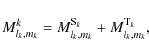
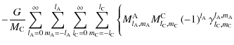
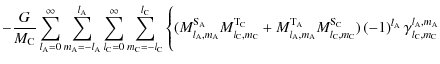
Inserting Eqs. (115) into (114), the respective Fourier expansions of
,
 and
are derived:
and
are derived:
 |
= |  |
|
![$\displaystyle \times{ \frac{1}{a_{\rm C}^{l_{\rm A}+l_{\rm C}+1}}\sum_{v,w,b}\k...
...eft[{\rm i}\Psi_{l_{\rm A}+l_{\rm C},m_{\rm A}+m_{\rm C},v,w,b}\right]\Bigg\}},$](/articles/aa/full_html/2009/15/aa9054-07/img361.png) |
(117) |
 |
= |  |
|
![$\displaystyle \times{ \frac{1}{a_{\rm C}^{l_{\rm A}+l_{\rm C}+1}}\sum_{v,w,b}\k...
...left[{\rm i}\Psi_{l_{\rm A}+l_{\rm C},m_{\rm A}+m_{\rm C},v,w,b}\right]\Bigg\}}$](/articles/aa/full_html/2009/15/aa9054-07/img364.png) |
(118) |
and
 |
= | |
|
![$\displaystyle \times{ \frac{1}{a_{\rm C}^{l_{\rm A}+l_{\rm C}+1}}\sum_{v,w,b}\k...
...eft[{\rm i}\Psi_{l_{\rm A}+l_{\rm C},m_{\rm A}+m_{\rm C},v,w,b}\right]\Bigg\}}.$](/articles/aa/full_html/2009/15/aa9054-07/img366.png) |
(119) |
This classification of the three different types of interaction allows us to explicitly generalize the classical case where the only considered extended body is the tidally perturbed one, A, while B and C are considered as punctual masses. In this case, the interaction are restricted to the classical gravitational interaction between
 ,
,
 ,
,
the mass of B, and .
,
,
the mass of B, and .
By now, to lighten the equations, the tidal multipole moments of C are ignored. In a practical case, they have to be derived using Eqs. (108), (109) and taken into account.
The disturbing function
is thus reduced to the two first interactions: the respective structural moments of body A and of body C and the structural moments of body C with the tidal moments of body A. The Fourier expansion of the disturbing function is thus given by
 |
(120) |
where
with
![$\displaystyle \times\frac{1}{a_{\rm C}^{l_{\rm A}+l_{\rm C}+1}} \sum_{v,w,b}\ka...
...ht)\exp\left[{\rm i}\Psi_{l_{\rm A}+l_{\rm C},m_{\rm A}+m_{\rm C},v,w,b}\right]$](/articles/aa/full_html/2009/15/aa9054-07/img373.png)
and
![$\displaystyle \times \frac{1}{a_{\rm C}^{l_{\rm A}+l_{\rm C}+1}}\sum_{v,w,b}\ka...
...t)\exp\left[{\rm i}\Psi_{l_{\rm A}+l_{\rm C},m_{\rm A}+m_{\rm C},v,w,b}\right].$](/articles/aa/full_html/2009/15/aa9054-07/img376.png)
Using Eq. (105), the tide-structure interaction disturbing function is expanded as
where
 and
and
 respectively correspond to the
and
contribution to the external gravitational potential of the tidally perturbed body A,
.
Inserting the explicit expansion for
and
given in Eqs. (108) and (109) into (123), we get
respectively correspond to the
and
contribution to the external gravitational potential of the tidally perturbed body A,
.
Inserting the explicit expansion for
and
given in Eqs. (108) and (109) into (123), we get
where
:

where
 and
and
 correspond to the adiabatic response of A. Finally, as in Eq. (43)
3.3 Dynamical equations
The external potential of the tidally perturbed body A by a body B being now well understood and known, our purpose here is to derive the dynamical equations for the evolution of the angular velocity (the angular momentum in term of Andoyer's variables) and the obliquity of A under the action of the gravitational interaction with a body C, which could be different from the perturber B and of the Keplerian orbital elements of this third body: ,
,
and .
To achieve this, we follow the method adopted by Yoder (1995, 1997) and Correia & Laskar (2003-c), who used the mutual interaction potential for the variation in the Andoyer variables and the disturbing function of the orbital elements. Here, gravitational interactions between B and C are not taken into account.
Begining with the Andoyer variables (cf. Andoyer 1926), we respectively get the total angular momentum,
 ,
where
,
where  is the inertia momentum of A,
 |
(127) |
and the obliquity,
:
 |
(128) |
The classical equations of orbital evolution are given by the Lagrange planetary equations (cf. Brouwer & Clemence 1961):
 |
(129) |
 |
(130) |
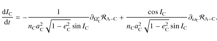 |
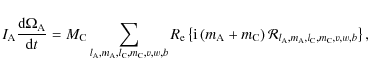
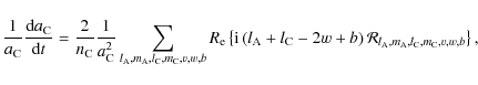
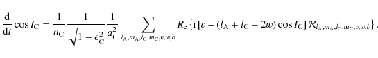
(131) |
The Fourier expansion of the disturbing function
is then introduced,
 |
(132) |
where, as in Eq. (114),
 is given by:
 |
= |  |
|
![$\displaystyle \times\frac{1}{a_{\rm C}^{l_{\rm A}+l_{\rm C}+1}}\kappa_{l_{\rm A...
...t)\exp\left[{\rm i}\Psi_{l_{\rm A}+l_{\rm C},m_{\rm A}+m_{\rm C},v,w,b}\right].$](/articles/aa/full_html/2009/15/aa9054-07/img406.png) |
(133) |
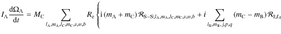
Therefore, the following formal equations are obtained for the dynamical evolution of respectively the angular velocity of A and its obliquity,
 |
(134) |
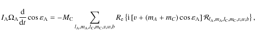 |
(135) |
where
 is the real part of a complex number or function z, while those for the Keplerian elements are given by
 |
(136) |
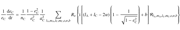 |
(137) |
and
 |
(138) |
If the tidal multipole moments of C are ignored, the following system is obtained using Eqs. (121) and (124) due to the dependence of
and
on
and
:
 | |||
![$\displaystyle {\left.+{\rm i}\sum_{l{'}_{\!\!\rm A},m{'}_{\!\!\rm A},l_{\rm B},...
...L_{\rm I\!I}}\right]{\mathcal R}_{{\rm I\!I}; L_{\rm I\!I}}^{\rm Ad}\right\}} ,$](/articles/aa/full_html/2009/15/aa9054-07/img414.png) |
(139) | ||
![$\displaystyle {I_{\rm A}\Omega_{\rm A}\frac{{\rm d}}{{\rm d}t}\cos\varepsilon_{...
...]{\mathcal R}_{{\rm S}-{\rm S};l_{\rm A},m_{\rm A},l_{\rm C},m_{\rm C},v,w,b} }$](/articles/aa/full_html/2009/15/aa9054-07/img415.png) | |||
![$\displaystyle -{\rm i}\sum_{l_{\rm B},m_{\rm B},j,p,q}\left[\left(v-j\right)+\l...
...ht)\right)\cos\varepsilon_{\rm A}\right]{\mathcal R}_{{\rm I\!I}; L_{\rm I\!I}}$](/articles/aa/full_html/2009/15/aa9054-07/img416.png) |
|||
![$\displaystyle { +\sum_{l_{\rm B},m_{\rm B},j,p,q}\left[\left(\partial_{\phi_{\r...
...A},L_{\rm I\!I}}\right]{\mathcal R}_{{\rm I\!I}; L_{\rm I\!I}}^{\rm Ad}\Bigg\}}$](/articles/aa/full_html/2009/15/aa9054-07/img417.png) |
(140) | ||
and
![$\displaystyle {\frac{1}{a_{\rm C}}\frac{{\rm d}a_{\rm C}}{{\rm d}t}=\frac{2}{n_...
..._{\rm B},m_{\rm B},r,s,u}{\mathcal R}_{{\rm I\!I}; L_{\rm I\!I}}\right]\right.}$](/articles/aa/full_html/2009/15/aa9054-07/img418.png) | |||
![$\displaystyle {\left.+\sum_{l_{\rm B},m_{\rm B},j,p,q}\partial_{M_{\rm C}}\left...
...L_{\rm I\!I}}\right]{\mathcal R}_{{\rm I\!I}; L_{\rm I\!I}}^{\rm Ad}\right\}} ,$](/articles/aa/full_html/2009/15/aa9054-07/img419.png) |
(141) | ||
 | |||
![$\displaystyle \times \sum_{l_{\rm A},m_{\rm A},l_{\rm C},m_{\rm C},v,w,b}R_{\rm...
...l_{\rm B},m_{\rm B},r,s,u}{\mathcal R}_{{\rm I\!I}; L_{\rm I\!I}}\right]\right.$](/articles/aa/full_html/2009/15/aa9054-07/img421.png) |
|||
![$\displaystyle {\left.+\sum_{l_{\rm B},m_{\rm B},j,p,q}\left[\left(\partial_{M_{...
...,L_{\rm I\!I}}\right]{\mathcal R}_{{\rm I\!I}; L_{\rm I\!I}}^{\rm Ad}\right\}},$](/articles/aa/full_html/2009/15/aa9054-07/img422.png) |
(142) | ||
![$\displaystyle {\frac{{\rm d}}{{\rm d}t}\cos I_{\rm C}=\frac{1}{n_{\rm C}}\frac{...
..._{\rm B},m_{\rm B},r,s,u}{\mathcal R}_{{\rm I\!I}; L_{\rm I\!I}}\right]\right.}$](/articles/aa/full_html/2009/15/aa9054-07/img423.png) | |||
![$\displaystyle {\left.+\sum_{l_{\rm B},m_{\rm B},j,p,q}\left[\left(\partial_{{\O...
...},L_{\rm I\!I}}\right]{\mathcal R}_{{\rm I\!I}; L_{\rm I\!I}}^{\rm Ad}\right\}}$](/articles/aa/full_html/2009/15/aa9054-07/img424.png) |
(143) | ||
where the explicit expression for
and
have been derived in Eqs. (122), (125), and (126).
4 Scaling laws in the case of an extended axisymmetric deformed perturber
4.1 Comparison to the punctual case
Here, our goal is to quantify the term(s) of the disturbing function due to the non-punctual behavior of the perturber B and to compare it to the one in the punctual mass case.
To achieve this aim, some assumptions are assumed. First, we adopt the quadrupolar approximation for the response of A to the tidal excitation by B; thus, we put
 so that
 .
Then, we consider the simplified situation where the body of which dynamics is studied is the tidal perturber; therefore, B = C and Eq. (125) becomes
.
Then, we consider the simplified situation where the body of which dynamics is studied is the tidal perturber; therefore, B = C and Eq. (125) becomes
 |
= | ![$\displaystyle -\frac{G}{M_{\rm B}}\frac{4\pi}{5}k_{2}^{\rm A}R_{\rm A}^5\left\v...
...{2,m_{\rm A}}\right]^2\left\vert M_{l_{\rm B},m_{\rm B}}^{\rm B} \right\vert ^2$](/articles/aa/full_html/2009/15/aa9054-07/img428.png) |
|
![$\displaystyle \times\frac{1}{a_{\rm B}^{2\left(2+l_{\rm B}+1\right)}}\left[\kap...
... B}\right)\right]^{2}\left[G_{2+l_{\rm B},p,q}\left(e_{\rm B}\right)\right]^{2}$](/articles/aa/full_html/2009/15/aa9054-07/img429.png) |
|||
| (144) |
On the other hand, since we are interested in the amplitude of
,
we focus on its norm (
 ). Finally, as we know that the dissipative part of the tide is very small compared to the adiabatic one (cf. Zahn 1966a), we can assume that
 in this first step.
Let us first derive the term of
due to the non-punctual term of the gravific potential of B, which has a non-zero average in time over an orbital period of B,
![]() that corresponds to the axisymmetric rotational and permanent tidal deformations (see Zahn 1977). (The same procedure can of course be applied to the non-stationary and non-axisymmetric deformations, but we choose here to focus only on
that corresponds to the axisymmetric rotational and permanent tidal deformations (see Zahn 1977). (The same procedure can of course be applied to the non-stationary and non-axisymmetric deformations, but we choose here to focus only on
 to illustrate our purpose.) Then, as the considered deformations of B are axisymmetric, we can expand them using the usual gravitational moments of B (
 )
as
)
as
 |
(145) |
Then, we obtain
![\begin{displaymath}\left\vert{\mathcal R}_{{\rm I};L_{\rm I}}^{J_{l_{\rm B}}}\le...
...{2}\left[G_{2+l_{\rm B},p,q}\left(e_{\rm B}\right)\right]^{2}.
\end{displaymath}](/articles/aa/full_html/2009/15/aa9054-07/img437.png)
On the other hand, the term of
associated to ,
namely the disturbing function in the case where B is assumed to be a punctual mass, is given by
![$\displaystyle \frac{G}{M_{\rm B}}\frac{4\pi}{5}k_{2}^{\rm A}R_{\rm A}^5 \left[\...
...eft(I_{\rm B}\right)\right]^{2}\left[G_{2,p,q}\left(e_{\rm B}\right)\right]^{2}$](/articles/aa/full_html/2009/15/aa9054-07/img439.png)
![$\displaystyle \frac{G}{M_{\rm B}}\frac{4\pi}{5}k_{2}^{\rm A}R_{\rm A}^5 M_{\rm ...
...t(I_{\rm B}\right)\right]^{2}\left[G_{2,p,q}\left(e_{\rm B}\right)\right]^{2} .$](/articles/aa/full_html/2009/15/aa9054-07/img440.png)
For this first evaluation of the ratio
 ,
we focus on the configuration of minimum energy. In this state, the spins of A and B are aligned with the orbital one so that
,
we focus on the configuration of minimum energy. In this state, the spins of A and B are aligned with the orbital one so that
 (that leads to
 and
and
 ). Then, we consider
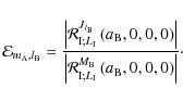 |
(148) |
Using Eqs. (146), (147), we get its expression in function of
and of
 :
:
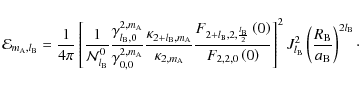 |
(149) |
As emphasized by Zahn (1966a, 1977), the main mode of the dissipative tide ruling the secular evolution of the system is
 .
We thus define
.
We thus define
 ,
such that
,
such that
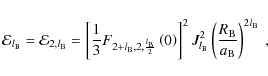 |
(150) |
which can be recast into
![\begin{displaymath}\log\left({\mathcal E}_{l_{\rm B}}\right)=2\left[\log\left[\f...
...\rm B}\log\left(\frac{a_{\rm B}}{R_{\rm B}}\right)\right]\cdot
\end{displaymath}](/articles/aa/full_html/2009/15/aa9054-07/img452.png) |
(151) |
Finally, taking only the quadrupolar deformation of B (J2) into account, we get
![\begin{displaymath}\log\left({\mathcal E}_{2}\right)=2\left[\log\left(\frac{5}{2...
...{2}-2\log\left(\frac{a_{\rm B}}{R_{\rm B}}\right)\right] \cdot
\end{displaymath}](/articles/aa/full_html/2009/15/aa9054-07/img453.png)
This gives us the order of magnitude of the terms due to the non-punctual behavior of B compared to the one obtained in the punctual mass approximation. It is directly proportional to the squarred J2, thus increasing with
 (where
 with
with
 )
in the case of the rotation-induced deformation and with
)
in the case of the rotation-induced deformation and with
 (where
 where
where
 )
in the tidal one, while it increases as
)
in the tidal one, while it increases as
 .
Therefore, as it is shown in Fig. 5, the non-punctual terms have to be taken into account for strongly deformed perturbers (
)
in very close systems (
), while they decrease rapidly otherwise. This corresponds for example to the case of internal natural satellites of rapidly rotating giant planets such as Jupiter and Saturn (
.
Therefore, as it is shown in Fig. 5, the non-punctual terms have to be taken into account for strongly deformed perturbers (
)
in very close systems (
), while they decrease rapidly otherwise. This corresponds for example to the case of internal natural satellites of rapidly rotating giant planets such as Jupiter and Saturn (
![\begin{figure}
\par\includegraphics[width=12cm,clip]{9054fig5.eps}
\end{figure}](/articles/aa/full_html/2009/15/aa9054-07/img464.png) |
Figure 5:
|
| Open with DEXTER | |
 as a function of
 for
J2=10-3 (red dashed line), 10-2 (purple long-dashed line), 10-1 (blue solid line). The non-punctual terms have to be taken into account for strongly deformed perturbers (
for
J2=10-3 (red dashed line), 10-2 (purple long-dashed line), 10-1 (blue solid line). The non-punctual terms have to be taken into account for strongly deformed perturbers (
4.2 Application to rapidly rotating binary stars
Here, we apply the previous procedure to the case of rapidly rotating binary stars where
 .
First, we roughly scale J2 of B to
.
First, we roughly scale J2 of B to  as (cf. Roxburgh 2001)
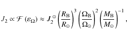 |
(153) |
the deformation being thus mainly due to rotation. Then, Eq. (152) becomes
![\begin{displaymath}\log\left({\mathcal E}_{2}\right)\approx2\left[\log\left(\fra...
...ght)-2\log\left(\frac{a_{\rm B}}{R_{\rm B}}\right)\right]\cdot
\end{displaymath}](/articles/aa/full_html/2009/15/aa9054-07/img468.png) |
(154) |
Then, we introduce the stellar homology relations for main-sequence stars (cf. Kippenhahn & Weigert 1990):
 |
(155) |
where
 is the nuclear energy production rate per unit mass inside the star. We finally obtain
|
(156) |
For main-sequence stars burning their hydrogen
 ,
while considering the pp chains leads to
,
while considering the pp chains leads to
 (
(
 )
and the CNO cycle to
)
and the CNO cycle to
 (
(
 )
(see Kippenhahn & Weigert 1990, for a detailed discussion).
)
(see Kippenhahn & Weigert 1990, for a detailed discussion).
In Fig. 6, we plot
 as a function of
 and
and
 for
for
 taking
 .
It is shown that the non-punctual terms are not always a perturbation compared to the punctual mass one (
.
It is shown that the non-punctual terms are not always a perturbation compared to the punctual mass one (
 )
for
)
for
 and
and
 that corresponds to rapidly rotating close binary massive stars. This has to be taken into account in future studies dedicated to the evolution of such stars.
![\begin{figure}
\par\includegraphics[width=12cm,clip]{9054fig6.eps}
\end{figure}](/articles/aa/full_html/2009/15/aa9054-07/img483.png) |
Figure 6:
|
| Open with DEXTER | |
 (red dashed line), 40
 Since we now have identified the regime where the non-punctual terms have to be taken into account, those have to be examined by integrating the complete set of dynamical equations. This will be presented in a forthcoming paper.
5 Conclusion
This work represents another step towards modeling the tidal dynamical evolution of planetary systems and of multiple stars by taking the extended character of the bodies into account. We have used the STF tensors that allow us to analytically and compactly treat the complex couplings between the multipole behavior of the gravitational fields of two extended bodies. First, the main properties of STF tensors were defined and derived. Next, after deriving the classical multipole expansion of the self gravitational field of an extended body A, we have derived the tidal potential related to the interaction between two extended bodies A and B, which is a generalization of the previous results where the perturber is treated through the punctual mass approximation. Using those results, the external potential of a tidally-perturbed body was provided and used to obtain the associated mutual interaction potential with a body C for which the dynamics is studied and which could be different from the previous tidal perturber B, as well as the corresponding disturbing function. Once the disturbing function were expanded into Fourier's series, the dynamical equations were derived. Those allows us to study the dynamical evolution of the angular momentum and the obliquity of the body A simultaneously with the Keplerian orbital elements of C relative to the center of mass of A, namely the semi major axis, ,
the eccentricity, ,
and the orbital inclination, .
The equations were derived in a general way without any linearization of function of any orbital elements as it has been done in Hut (1981, 1982) and in Correia & Laskar (2003b). This allowed us to study the strongly nonlinear problem of inclined, eccentric orbits. Therefore, this formalism can be useful for elliptic systems.
The major interest of this modeling concerns the dissipation of the tidal mechanical energy. Here, the response of each extended body is parametrized through the Love number kl for the adiabatic one, and an impedance  and its associated delay
 ,
which describes the damping and the phase lag due to the (viscous and thermal) dissipation acting on the bulk-induced by the perturber. Self-consistent modellings have to be developed for elasto-viscous bodies (Rogister & Rochester 2004), for fluid bodies (cf. Zahn 1977), and equilibrium and stability conditions. This will be done for extended fluid bodies in a forthcoming series of papers.
,
which describes the damping and the phase lag due to the (viscous and thermal) dissipation acting on the bulk-induced by the perturber. Self-consistent modellings have to be developed for elasto-viscous bodies (Rogister & Rochester 2004), for fluid bodies (cf. Zahn 1977), and equilibrium and stability conditions. This will be done for extended fluid bodies in a forthcoming series of papers.
Moreover, due to the general character of this work, various applications are possible. The first one deals with the dynamics of planets that are very close to their star, as observed in several extrasolar planetary systems (cf. Laskar & Correia 2004; Levrard et al. 2007; Fabrycky et al. 2007; Correia et al. 2008). Next, in our own Solar System, dynamical systems, such as giant planets and their internal satellites, can be studied by taking their spatial extension and their multipolar behavior into account, due for example to their rapid rotation. Finally, this work can be applied to the dynamical evolution of close binary stars where the tidal interaction and its dissipation dominate the behavior of the system until it has reached its lower energy state, where the spins are all aligned, the orbits are circular, and the components are synchronized with the orbital motion. For these future applications, the potential impact of the spatial extension of bodies on dynamics has to be carefully evaluated and understood.
Acknowledgements
It is a real pleasure to acknowledge Pr. J.-P. Zahn, Pr. T. Damour, and Dr. J. Vaubaillon for helpful comments. We are also grateful to the anonymous referee for her or his suggestions that allowed us to improve the original manuscript.
References
- Abramowitz, M., & Stegun, I. 1972, Handbook of mathematical functions (New York: Dover) (In the text)
- Alexander, M. E. 1973, Ap&SS, 23, 459 [NASA ADS] [CrossRef] (In the text)
- Andoyer, H. 1926, Mécanique Céleste (Paris: Gauthier-Villars) (In the text)
- Blanchet, L., & Damour, T. 1986, Phil. Trans. R. Soc. Lon. A, 320, 379 [NASA ADS] [CrossRef] (In the text)
- Bordé, P., Rouan, D., & Léger, A. 2003, 405, 1137
- Borderies, N. 1978, Celest. Mech., 18, 295 [NASA ADS] [CrossRef] (In the text)
- Borderies, N. 1980, A&A, 82, 129 [NASA ADS] (In the text)
- Borderies, N., & Yoder, C. F. 1990, A&A, 233, 235 [NASA ADS] (In the text)
- Borucki, W. J., Koch, D. G., Lissauer, J., et al. 2007, Transiting Extrasolar Planets, Proceedings of the conference held 25-28 September 2006 at the Max Planck Institute for Astronomy in Heidelberg, Germany, ed. C. Afonso, D. Weldrake, & Th. Henning (San Francisco: ASP), ASP Conf. Ser., 366, 309
- Brouwer, D., & Clemence, G. M. 1961, Methods of celestial mechanics (New York: Academic Press) (In the text)
- Correia, A. C. M. 2001, Ph. D. Thesis, Université Paris VII (In the text)
- Correia, A. C. M., & Laskar, J. 2001, Nature, 411 (Issue 6839), 767
- Correia, A. C. M., & Laskar, J. 2003a, Icarus, 163, 24 [NASA ADS] [CrossRef]
- Correia, A. C. M., & Laskar, J. 2003b, J. Geophys. Res., 108 (Issue E11), 5123 (In the text)
- Correia, A. C. M., Laskar, J., & Néron de Surgy, O. 2003, Icarus, 163, 1 [NASA ADS] [CrossRef] (In the text)
- Correia, A. C. M., Levrard, B., & Laskar, J. 2008, A&A, 488, L63 [NASA ADS] [CrossRef] [EDP Sciences] (In the text)
- Courant, R., & Hilbert, D. 1953, Methods of Mathematical Physics (New York: Interscience) (In the text)
- Damour, T., Soffel, M. H., & Xu, C. 1992, Phys. Rev. D, 45, 1017 [NASA ADS] [CrossRef] (In the text)
- Fabrycky, D. C., Johnson, E. T., & Goodman, J. 2007, ApJ, 665, 754 [NASA ADS] [CrossRef] (In the text)
- Gelfand, I. M., Minlos, R. A., & Shapiro, Z. Ya. 1963, Representation of the Rotation of the Lorentz groups (Oxford: Pergamon) (In the text)
- Guillot, T. 1999, Planet. Space Sci., 47, 1183 [NASA ADS] [CrossRef] (In the text)
- Hartmann, T., Soffel, M. H., & Kioustelidis, T. 1994, Celest. Mech. Dyn. Astron., 60, 139 [NASA ADS] [CrossRef] (In the text)
- Hut, P. 1981, A&A, 99, 126 [NASA ADS] (In the text)
- Hut, P. 1982, A&A, 110, 37 [NASA ADS] (In the text)
- Ilk, K. H. 1983, Ph.D. Thesis, Technischen Universitaet, Munich Bayerische Akademie der Wissenschaften (In the text)
- Kaula, W. M. 1962, AJ, 67, 300 [NASA ADS] [CrossRef] (In the text)
- Kippenhahn, R., & Weigert, W. 1990, Stellar Structure and Evolution (Springer) (In the text)
- Lambeck, K. 1980, The Earth's Variable Rotation (Cambridge University Press) (In the text)
- Levrard, B., Correia, A. C. M., Chabrier, G., et al. 2007, A&A, 462, L5 [NASA ADS] [CrossRef] [EDP Sciences] (In the text)
- Laskar, J. 2005, Celest. Mech. Dyn. Astron., 91, 351 [NASA ADS] [CrossRef] (In the text)
- Laskar, J., & Correia, A. C. M. 2004, Extrasolar Planets: Today and Tomorrow, ed. J.-P. Beaulieu, A. Lecavelier des Etangs, & C. Terquem, ASP Conf. Proc., 321, 401 (In the text)
- Maciejewski, A. J. 1995, Celest. Mech. Dyn. Astron., 63, 1 [NASA ADS] [CrossRef] (In the text)
- Mayor, M., Pont, F., & Vidal-Madjar, A. 2005, Progr. Theor. Phys. Suppl., 158, 43 [NASA ADS] [CrossRef] (In the text)
- Melchior, P. J. 1971, Physique et dynamique planétaire (Bruxelles: Vander) (In the text)
- Néron de Surgy, O. 1996, Ph.D. Thesis, Observatoire de Paris (In the text)
- Néron de Surgy, O., & Laskar, J. 1997, A&A, 318, 975 [NASA ADS] (In the text)
- Rogister, Y., & Rochester, M. G. 2004, Geophys. J. Inter., 159, 874 [NASA ADS] [CrossRef] (In the text)
- Roxburgh, I. W. 2001, A&A, 377, 688 [NASA ADS] [CrossRef] [EDP Sciences] (In the text)
- Thorne, K. 1980, Rev. Mod. Phys., 52, 299 [NASA ADS] [CrossRef] (In the text)
- Tisserand, F. F. 1889, Traité de Mécanique Céleste Tome I (Paris: Gauthier Villars) (In the text)
- Tisserand, F. F. 1891, Traité de Mécanique Céleste Tome II (Paris: Gauthier Villars) (In the text)
- Yoder, C. F. 1995, Icarus, 117, 250 [NASA ADS] [CrossRef] (In the text)
- Zahn, J.-P. 1966a, Annales d'Astrophysique, 29, 313 [NASA ADS]
- Zahn, J.-P. 1966b, Annales d'Astrophysique, 29, 489 [NASA ADS]
- Zahn, J.-P. 1977, A&A, 57, 383 [NASA ADS] (In the text)
Footnotes
- ...
![[*]](/icons/foot_motif.png)
- They are driven by two types of deformation. The first one is those induced by internal dynamical processes such that rotation (through the centrifugal acceleration) and magnetic field (through the volumetric Lorentz force). The second one is the axisymmetric permanent tidal oval shape due to a companion in close binary or multiple systems.
- ... potential
- The denomination of
 as a potential is not very pertinent since it has the dimension of the product of a mass by a potential. However, we keep it to stay coherent with Hartmann et al. (1994).
- ... mode
- Note that each tidal Fourier mode has its own dissipation rate as shown by Zahn (1966b, 1977).
- ...
- The tidal multipole moments of B due to A can be derived using the same methodology and substituting A to B for the perturber and vice versa.
All Tables
Table 1:
Values of the obliquity function
![]() in the case where l=2 and
in the case where l=2 and ![]() obtained from Eq. (81) (adapted from Yoder 1995).
obtained from Eq. (81) (adapted from Yoder 1995).
Table 2:
Values of the inclination function
![]() in the case where l=2, and values for j<0 can be deduced from Eq. (86) (adapted from Lambeck 1980).
in the case where l=2, and values for j<0 can be deduced from Eq. (86) (adapted from Lambeck 1980).
Table 3:
Values of the eccentricity function
![]() in the case where l=2 (adapted from Lambeck 1980), where several combinations
in the case where l=2 (adapted from Lambeck 1980), where several combinations
![]() have the same Gl,p,q value.
have the same Gl,p,q value.
All Figures
| |
Figure 1:
System of two extended bodies.
|
| Open with DEXTER | |
| In the text | |
| |
Figure 2:
Spherical coordinate system associated to the equatorial reference frame
|
| Open with DEXTER | |
| In the text | |
| |
Figure 3:
Inertial reference, orbital, and equatorial rotating frames (
|
| Open with DEXTER | |
| In the text | |
| |
Figure 4:
Classical tidal dynamical system. The extended body B is tidally disturbing the extended body A, which adjusts with a phase lag
|
| Open with DEXTER | |
| In the text | |
| |
Figure 5:
|
| Open with DEXTER | |
| In the text | |
| |
Figure 6:
|
| Open with DEXTER | |
| In the text | |
Copyright ESO 2009
Current usage metrics show cumulative count of Article Views (full-text article views including HTML views, PDF and ePub downloads, according to the available data) and Abstracts Views on Vision4Press platform.
Data correspond to usage on the plateform after 2015. The current usage metrics is available 48-96 hours after online publication and is updated daily on week days.
Initial download of the metrics may take a while.