| Issue |
A&A
Volume 497, Number 3, April III 2009
|
|
|---|---|---|
| Page(s) | L17 - L20 | |
| Section | Letters | |
| DOI | https://doi.org/10.1051/0004-6361/200811502 | |
| Published online | 19 March 2009 | |
LETTER TO THE EDITOR
Relationship between photospheric currents and coronal magnetic helicity for force-free bipolar fields
S. Régnier
School of Mathematics and Statistics, University of St Andrews, St Andrews, Fife, KY16 9SS, UK
Received 11 December 2008 / Accepted 13 March 2009
Abstract
Aims. The origin and evolution of the magnetic helicity in the solar corona are not well understood. For instance, the magnetic helicity of an active region is often about 1042 Mx2 (1026 Wb2), but the observed processes whereby it is thought to be injected into the corona do not yet provide an accurate estimate of the resulting magnetic helicity budget or time evolution. The variation in magnetic helicity is important for understanding the physics of flares, coronal mass ejections, and their associated magnetic clouds. To shed light on this topic, we investigate here the changes in magnetic helicity due to electric currents in the corona for a single twisted flux tube that may model characteristic coronal structures such as active region filaments, sigmoids, or coronal loops.
Methods. For a bipolar photospheric magnetic field and several distributions of current, we extrapolated the coronal field as a nonlinear force-free field. We then computed the relative magnetic helicity, as well as the self and mutual helicities.
Results. Starting from a magnetic configuration with a moderate amount of current, the amount of magnetic helicity can increase by 2 orders of magnitude when the maximum current strength is increased by a factor of 2. The high sensitivity of magnetic helicity to the current density can partially explain discrepancies between measured values on the photosphere, in the corona, and in magnetic clouds. Our conclusion is that the magnetic helicity strongly depends on both the strength of the current density and also on its distribution.
Conclusions. Only improved measurements of current density at the photospheric level will advance our knowledge of the magnetic helicity content in the solar atmosphere.
Key words: Sun: corona - Sun: magnetic fields - Sun: flares - Sun: coronal mass ejections (CMEs)
1 Introduction
Magnetic helicity is an important quantity in the physics of eruptive events occurring in the solar corona. Active region filaments and sigmoids have been observed and modelled as twisted flux bundles (Gibson et al. 2002; Török & Kliem 2003; Canfield et al. 1999; Aulanier & Démoulin 1998; Régnier & Amari 2004; Rust & Kumar 1996; Aulanier et al. 1999; Régnier et al. 2002). Magnetic helicity is also thought to play an important role in the formation of filaments (e.g., Mackay et al. 1997; Mackay & van Ballegooijen 2005) and possibly in coronal heating (e.g., Priest 1999; Heyvaerts & Priest 1984). The instability of coronal structures is related to the amount of helicity stored in the magnetic field and the possible transfer of twist to writhe or self helicity from mutual helicity.
Nevertheless, only proxies of the magnetic helicity have been used to estimate the twist of magnetic structures. In Leamon et al. (2004), the linear force-free parameter  was derived as a proxy for the twist of coronal structures observed in X-rays based on the thin flux tube approximation. The
twist values of the coronal structures and of the associated magnetic clouds are inconsistent, suggesting that the propagation of coronal mass ejections (CMEs) in the corona involves a transfer between the mutual helicity of the overlying field and the self helicity of the flux rope. Based on a linear force-free assumption, Démoulin et al. (2002) have shown that the helicity of magnetic clouds is
comparable to the end-to-end helicity of the twisted bundle formed in the associated active region. This suggests that the helicity is more likely to be injected through the photosphere by flux emergence or localized magnetic field motions (see also Welsch & Longcope 2003; Kusano et al. 2002; Longcope et al. 2007; Chae 2001; Magara & Longcope 2003). The helicity injection processes play a key role in the long-term evolution of solar magnetic field (e.g., Yeates et al. 2008). The helicity of magnetic clouds, however, is often found to be one or two orders of magnitude greater than the estimated coronal helicity. In this Letter, we model coronal structures by a single twisted flux tube with several distributions of current density and study the variations in the helicity content due to an increase in current density.
was derived as a proxy for the twist of coronal structures observed in X-rays based on the thin flux tube approximation. The
twist values of the coronal structures and of the associated magnetic clouds are inconsistent, suggesting that the propagation of coronal mass ejections (CMEs) in the corona involves a transfer between the mutual helicity of the overlying field and the self helicity of the flux rope. Based on a linear force-free assumption, Démoulin et al. (2002) have shown that the helicity of magnetic clouds is
comparable to the end-to-end helicity of the twisted bundle formed in the associated active region. This suggests that the helicity is more likely to be injected through the photosphere by flux emergence or localized magnetic field motions (see also Welsch & Longcope 2003; Kusano et al. 2002; Longcope et al. 2007; Chae 2001; Magara & Longcope 2003). The helicity injection processes play a key role in the long-term evolution of solar magnetic field (e.g., Yeates et al. 2008). The helicity of magnetic clouds, however, is often found to be one or two orders of magnitude greater than the estimated coronal helicity. In this Letter, we model coronal structures by a single twisted flux tube with several distributions of current density and study the variations in the helicity content due to an increase in current density.
In reconstructed magnetic fields, the magnetic energy increases when the current density is increased; however, we can only inject a finite amount of current into a finite domain of computation. An upper limit of the amount of free magnetic energy is given by the Aly-Sturrock (AS) limit (Aly 1984; Sturrock 1991) stating that, for a magnetic field strength decaying fast enough at infinity in the half space above the photosphere, the magnetic energy of the open magnetic field is the least upper bound of the magnetic energy of a force-free field. Thus, the magnetic helicity that can be injected into a magnetic configuration is also bounded. The magnetic energy of the open field configuration is about twice the magnetic energy of the potential field (e.g., Amari et al. 2000). Both the potential field energy and open field energy depend of the total unsigned flux magnetic field through the surface. In a finite domain of computation as is the case for magnetic field extrapolations, the AS limit is used to check the validity of a magnetic configuration, therefore the extrapolated configuration is considered valid when the magnetic energy of the force-free field is lower than the magnetic energy of the open field. This condition is true when closed boundary conditions are used to derive the nonlinear force-free field.
2 Magnetic field and current distributions
The first step in order to derive the magnetic helicity content in the corona is to compute the 3D magnetic field in a finite volume. We assume that the coronal magnetic field is described well by a nonlinear force-free field satisfying the following equations:
 ,
where is the force-free function depending on the position, and
,
where is the force-free function depending on the position, and
 ,
which implies that is a constant along a given field line. The
magnetic field also has to satisfy the solenoidal condition (
,
which implies that is a constant along a given field line. The
magnetic field also has to satisfy the solenoidal condition (
 ). We solve this problem in accordance with the method developed by Grad & Rubin (1958). Following Sakurai (1981), the boundary conditions for solving this set of equations as a mathematically
well-posed boundary problem are the vertical component of the magnetic field everywhere on the surface
). We solve this problem in accordance with the method developed by Grad & Rubin (1958). Following Sakurai (1981), the boundary conditions for solving this set of equations as a mathematically
well-posed boundary problem are the vertical component of the magnetic field everywhere on the surface
 ,
and the distribution of
in one chosen polarity on
,
and the distribution of
in one chosen polarity on
 .
We use the numerical scheme developed by Amari et al. (1999,1997), which was successfully applied to solar active regions by Régnier et al. (2002, 2004, 2006) by qualitatively comparing the computed field lines to multi-wavelength observations. It is important to note that we use closed boundary conditions on the sides of the computational box, different from the bottom boundary, which are compatible
with the boundary conditions used to derive the helicity integrals (see Sect. 3).
.
We use the numerical scheme developed by Amari et al. (1999,1997), which was successfully applied to solar active regions by Régnier et al. (2002, 2004, 2006) by qualitatively comparing the computed field lines to multi-wavelength observations. It is important to note that we use closed boundary conditions on the sides of the computational box, different from the bottom boundary, which are compatible
with the boundary conditions used to derive the helicity integrals (see Sect. 3).
The second step is to define the appropriate boundary conditions on the bottom boundary: the vertical magnetic field on the surface and the distribution of the force-free function
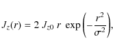
in one chosen polarity. As depicted in Fig. 1 left, the vertical magnetic field on the bottom boundary is a bipolar field embedded in a large field-of-view in order to minimise the influence of the boundaries on the magnetic field configurations. The vertical magnetic field component Bz is described by a Gaussian distribution (see Fig. 1a) with a maximum field strength of 2000 G and a full-width at half-maximum (FWHM) of about 15 Mm. The field-of-view is 150  150 Mm2 with a spatial resolution of 1 Mm. The peak-to-peak separation of the polarities is about 30 Mm.
The vertical current distributions are defined in the positive polarity as follows:
- Constant:
is a constant (see Fig. 1b) corresponding to a linear force-free field. The current distribution is then a Gaussian distribution with the same FWHM as Bz and a maximum current density strength Jz0.
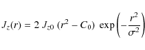
- Divided: the distribution is defined from a Hermite polynomial of 1st order dividing the polarity into a negative and a positive part (see Fig. 1c):
(1)
where r is the distance from the centre of the polarity. The current density flux through the positive polarity at the bottom boundary is then balanced. A free parameter of the current distribution is the angle between the polarity inversion line (PIL) and the current inversion line (CIL) in the positive polarity. We have chosen
 (with the negative currents towards the PIL) such that the magnetic energy is maximised.
- Ring: the vertical current density is defined as a Hermite polynomial of 2nd order in 1D:
(2)
where r is the distance from the centre of the polarity. A typical ring distribution is plotted in Fig. 1d with negative currents in the central region surrounded by positive currents. The constant C0 is such that the vertical current density in the positive polarity is balanced.
3 Helicity measurements
3.1 Magnetic helicities
The magnetic helicity describes the complexity of the field in terms of its topology, connectivity or braiding, and it is a measure of both the twist of field lines around the flux bundle axis and writhe of the axis itself (Berger 1999). The magnetic helicity is a conserved quantity in ideal MHD for a volume bounded by a surface on which the normal field component is fixed. However, the magnetic helicity is not conserved whilst modelling the solar corona above the photosphere since helicity may be injected from below the photosphere into the corona (e.g., Régnier & Canfield 2006) or it may be expelled in magnetic clouds during CMEs into the interplanetary medium.
![\begin{figure}
\par\mbox{\parbox[c]{4.5cm}{
\includegraphics[width=4.5cm]{1502fg...
...2cm]{1502fg1d.eps}
\includegraphics[width=2.2cm]{1502fg1e.eps}}} }\end{figure}](/articles/aa/full_html/2009/15/aa11502-08/img13.png) |
Figure 1:
Left: distribution of the vertical component of the magnetic field on the bottom boundary. The polarities are defined as Gaussian distributions with the same maximum strength in absolute value and the same FWHM. The field-of-view is 150 |
| Open with DEXTER | |
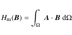
The magnetic helicity is defined as follows:
 |
(3) |
for a magnetic field
 and its vector potential
  in a volume
  .
The vector potential is not defined uniquely but depends on a gauge. Here we use a gauge-free expression of the
magnetic helicity due to Berger & Field (1984) and called the relative magnetic helicity
.
The vector potential is not defined uniquely but depends on a gauge. Here we use a gauge-free expression of the
magnetic helicity due to Berger & Field (1984) and called the relative magnetic helicity
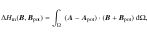 |
(4) |
where
and
describe the magnetic field of the configuration, and,
 and
and
 describe a reference field taken to be the potential field. We use the same boundary conditions as for the universal helicity formula derived by Hornig (2006).
Following Berger (1999), we define the self and mutual helicities as
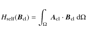 |
(5) |
and
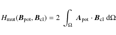 |
(6) |
when the field
can be decomposed into two fields, the reference field
and the closed field
 .
The boundary conditions are explained in Régnier et al. (2005) and they are the same as used to compute the nonlinear force-free field in this experiment.
.
The boundary conditions are explained in Régnier et al. (2005) and they are the same as used to compute the nonlinear force-free field in this experiment.
We note that those definitions of self and mutual helicities are different from the recent definitions given by Longcope & Malanushenko (2008). In the solar context, the self and mutual helicities as derived by Berger (1999) have been defined in Régnier et al. (2005) from measurements based on simple configurations and observed active regions. The self helicity is a measure of the twist and writhe of flux bundles confined in the coronal volume. The mutual helicity characterises the crossing of field lines and the large-scale twist.
3.2 Helicities vs. current
We now compute the nonlinear force-free field in the corona for the three different distributions of current, and we study the changes in the magnetic configurations caused by an increase in the maximum vertical current strength Jz0. In a forthcoming paper, we will extensively study the changes in the geometry of field lines, the magnetic connectivity, and the magnetic energy
budget. In this Letter, we focus our study on the changes in the magnetic helicity content of the bipolar field for the three different current distributions described in Sect. 2. The maximum current strength ranges from 0 to 24 mA m-2. We first plot the total unsigned current inside
as a function of Jz0 in Fig. 2 for the three current distributions. In Fig. 3, the self and mutual helicities are the blue and green
curves, respectively, whilst the total relative magnetic helicity is the red curve. We also indicate the AS limit when the magnetic energy of the nonlinear force-free field is 1.7 times the magnetic energy of the potential field, corresponding to the magnetic energy computed for the open
field. This upper limit gives
Jz0 = 6.6 mA m-2 for the constant distribution, 13.6 mA m-2 for the divided distribution. For this range of Jz0 values, there is no upper limit for the ring distribution, which indeed corresponds to a twisted flux bundle confined by return currents.
![\begin{figure}
\par\includegraphics[width=7.5cm,clip]{1502fg2.eps}
\end{figure}](/articles/aa/full_html/2009/15/aa11502-08/img24.png) |
Figure 2: Total unsigned current (A m) inside the computational volume as a function of the current density Jz0 for a constant distribution (dashed line), a divided distribution (dot-dashed line), and a ring distribution (solid line). |
| Open with DEXTER | |
The magnetic helicities have a positive sign, except for the relative magnetic helicity of the ring distribution below Jz0 = 5 mA m-2 (see Fig. 3c). From these computations, the mutual helicity values are most sensitive to the existence of an upper bound for the magnetic energy. For the constant and divided distributions (see Figs. 3a,b), the behaviour of the mutual helicity is strongly modified above the AS limit, whilst we get a smooth curve of mutual helicity for the ring distribution.
| |
Figure 3: Relative magnetic helicity (red solid line), self helicity (blue dot-dashed line), and mutual helicity (green dashed line) as a function of the maximum vertical current density Jz0 from 0 to 24 mA m-2 for a) a constant distribution; b) a divided distribution; c) a ring distribution. The helicities are expressed in units of 1040 G2 cm4. The straight dashed lines indicate the Aly-Sturrock limit. |
| Open with DEXTER | |
For all of the imposed current distributions, the magnetic helicity of the bipolar field is dominated by the self helicity, and thus the configurations are twisted flux tubes confined in a small domain of the computational box according to the definition given in Régnier et al. (2005). The helicity values vary from 1038 to 1042 G2 cm4 for the constant and divided distributions, from 1037 to 1041 G2 cm4 for the ring distributions. The ring distribution tends to reduce the amount of magnetic helicity stored in the confined twisted flux tube. The relative and self helicities show an exponential growth with increasing current density (linear trend in Fig. 3). For moderate values of the current density, these helicities vary by more than 1 order of magnitude when the current density Jz0 is multiplied by a factor of 2. For high values of Jz0, a plateau exists for all helicities. This suggests that instabilities such as kink instability can develop when the maximum helicity is reached inside the twisted flux bundle. The increase in magnetic helicity as a function of the total current is reduced compared to the evolution with respect to Jz0, but it is still significant depending on the distribution of Jz.
4 Discussion and conclusions
By modelling coronal magnetic structures by a bipolar field containing a single twisted flux tube, we have demonstrated that the magnetic helicity can vary by more than an order of magnitude when the current density is increased by a factor of 2. This shows that the departure from the potential field state has important consequences on the amount of magnetic helicity that can be stored in the corona, and therefore on the helicity content expelled during CMEs.
In terms of magnetic field modelling, we have shown that the behaviour of the magnetic helicity in a nonlinear force-free field strongly depends on the chosen distribution of current. If we inject a large amount of current density within the ring distribution, the magnetic helicity values are one order of magnitude lower than for the divided distribution as the twisted flux tube remains confined to a small fraction of the coronal volume. This is caused by the existence of return currents at the edges of the twisted flux bundle, whilst for the constant and divided current distributions, the field lines can expand towards the boundaries.
In terms of observation, the vertical current density is deduced from vector magnetic field measurements in the photosphere (or in the chromosphere):
![]() .
The uncertainties on the vertical current density strongly depend on the noise level of the transverse field components inverted from spectropolarimetric observations. From the above conclusions, it is worth noticing that magnetic helicity values in the corona obtained from photospheric observations have to be considered with caution as a small error on the measurement of the field components can dramatically change the value of the magnetic helicity. And so to better understand the physics of twisted flux bundles in the corona, it is important to improve the polarimetric resolution to increase the signal-to-noise ratio on the transverse field components and to increase the spatial resolution to resolve the current which is distributed on small scales
(e.g., Parker 1996). Even if the effects are weaker, these conclusions also apply to the change in helicity as a function of the total unsigned current.
.
The uncertainties on the vertical current density strongly depend on the noise level of the transverse field components inverted from spectropolarimetric observations. From the above conclusions, it is worth noticing that magnetic helicity values in the corona obtained from photospheric observations have to be considered with caution as a small error on the measurement of the field components can dramatically change the value of the magnetic helicity. And so to better understand the physics of twisted flux bundles in the corona, it is important to improve the polarimetric resolution to increase the signal-to-noise ratio on the transverse field components and to increase the spatial resolution to resolve the current which is distributed on small scales
(e.g., Parker 1996). Even if the effects are weaker, these conclusions also apply to the change in helicity as a function of the total unsigned current.
Acknowledgements
I thank E. R. Priest, D. Mackay, and G. Hornig for fruitful discussions. I thank the UK STFC for financial support (STFC RG). The computations were done using the XTRAPOL code developed by T. Amari (Ecole Polytechnique, France). I also acknowledge the financial support by the European Commission through the SOLAIRE network (MTRN-CT-2006-035484).
References
- Aly, J. J. 1984, ApJ, 283, 349 [NASA ADS] [CrossRef]
- Amari, T., Aly, J. J., Luciani, J. F., Boulmezaoud, T. Z., & Mikic, Z. 1997, Sol. Phys., 174, 129 [NASA ADS] [CrossRef] (In the text)
- Amari, T., Boulmezaoud, T. Z., & Mikic, Z. 1999, A&A, 350, 1051 [NASA ADS]
- Amari, T., Luciani, J. F., Mikic, Z., & Linker, J. 2000, ApJ, 529, L49 [NASA ADS] [CrossRef] (In the text)
- Aulanier, G., & Démoulin, P. 1998, A&A, 329, 1125 [NASA ADS]
- Aulanier, G., Démoulin, P., Mein, N., et al. 1999, A&A, 342, 867 [NASA ADS]
- Berger, M. A. 1999, in Measurement Techniques in Space Plasmas Fields, ed. M. R. Brown, R. C. Canfield, & A. A. Pevtsov, 1 (In the text)
- Berger, M. A., & Field, G. B. 1984, J. Fluid Mech., 147, 133 [NASA ADS] [CrossRef] (In the text)
- Canfield, R. C., Hudson, H. S., & McKenzie, D. E. 1999, Geophys. Res. Lett., 26, 627 [NASA ADS] [CrossRef]
- Chae, J. 2001, ApJ, 560, L95 [NASA ADS] [CrossRef]
- Démoulin, P., Mandrini, C. H., van Driel-Gesztelyi, L., et al. 2002, A&A, 382, 650 [NASA ADS] [CrossRef] [EDP Sciences] (In the text)
- Gibson, S. E., Fletcher, L., Del Zanna, G., et al. 2002, ApJ, 574, 1021 [NASA ADS] [CrossRef]
- Grad, H., & Rubin, H. 1958, in Proc. 2nd Int. Conf. on Peaceful Uses of Atomic Energy, Geneva, UN, 31, 190 (In the text)
- Heyvaerts, J., & Priest, E. R. 1984, A&A, 137, 63 [NASA ADS]
- Hornig, G. 2006, ArXiv Astrophysics e-prints (In the text)
- Kusano, K., Maeshiro, T., Yokoyama, T., & Sakurai, T. 2002, ApJ, 577, 501 [NASA ADS] [CrossRef]
- Leamon, R. J., Canfield, R. C., Jones, S. L., et al. 2004, J. Geophys. Res., Space Phys., 109, 5106 (In the text)
- Longcope, D. W., & Malanushenko, A. 2008, ApJ, 674, 1130 [NASA ADS] [CrossRef] (In the text)
- Longcope, D. W., Ravindra, B., & Barnes, G. 2007, ApJ, 668, 571 [NASA ADS] [CrossRef]
- Mackay, D. H., & van Ballegooijen, A. A. 2005, ApJ, 621, L77 [NASA ADS] [CrossRef]
- Mackay, D. H., Gaizauskas, V., Rickard, G. J., & Priest, E. R. 1997, ApJ, 486, 534 [NASA ADS] [CrossRef]
- Magara, T., & Longcope, D. W. 2003, ApJ, 586, 630 [NASA ADS] [CrossRef]
- Parker, E. N. 1996, ApJ, 471, 485 [NASA ADS] [CrossRef] (In the text)
- Priest, E. R. 1999, in Measurement Techniques in Space Plasmas Fields, ed. M. R. Brown, R. C. Canfield, & A. A. Pevtsov, 141
- Régnier, S., & Amari, T. 2004, A&A, 425, 345 [NASA ADS] [CrossRef] [EDP Sciences]
- Régnier, S., & Canfield, R. C. 2006, A&A, 451, 319 [NASA ADS] [CrossRef] [EDP Sciences] (In the text)
- Régnier, S., Amari, T., & Kersalé, E. 2002, A&A, 392, 1119 [NASA ADS] [CrossRef] [EDP Sciences]
- Régnier, S., Amari, T., & Canfield, R. C. 2005, A&A, 442, 345 [NASA ADS] [CrossRef] [EDP Sciences] (In the text)
- Rust, D. M., & Kumar, A. 1996, ApJ, 464, L199 [NASA ADS] [CrossRef]
- Sakurai, T. 1981, Sol. Phys., 69, 343 [NASA ADS] [CrossRef] (In the text)
- Sturrock, P. A. 1991, ApJ, 380, 655 [NASA ADS] [CrossRef]
- Török, T., & Kliem, B. 2003, A&A, 406, 1043 [NASA ADS] [CrossRef] [EDP Sciences]
- Welsch, B. T., & Longcope, D. W. 2003, ApJ, 588, 620 [NASA ADS] [CrossRef]
- Yeates, A. R., Mackay, D. H., & van Ballegooijen, A. A. 2008, Sol. Phys., 247, 103 [NASA ADS] [CrossRef] (In the text)
All Figures
| |
Figure 1:
Left: distribution of the vertical component of the magnetic field on the bottom boundary. The polarities are defined as Gaussian distributions with the same maximum strength in absolute value and the same FWHM. The field-of-view is 150 |
| Open with DEXTER | |
| In the text | |
| |
Figure 2: Total unsigned current (A m) inside the computational volume as a function of the current density Jz0 for a constant distribution (dashed line), a divided distribution (dot-dashed line), and a ring distribution (solid line). |
| Open with DEXTER | |
| In the text | |
| |
Figure 3: Relative magnetic helicity (red solid line), self helicity (blue dot-dashed line), and mutual helicity (green dashed line) as a function of the maximum vertical current density Jz0 from 0 to 24 mA m-2 for a) a constant distribution; b) a divided distribution; c) a ring distribution. The helicities are expressed in units of 1040 G2 cm4. The straight dashed lines indicate the Aly-Sturrock limit. |
| Open with DEXTER | |
| In the text | |
Copyright ESO 2009
Current usage metrics show cumulative count of Article Views (full-text article views including HTML views, PDF and ePub downloads, according to the available data) and Abstracts Views on Vision4Press platform.
Data correspond to usage on the plateform after 2015. The current usage metrics is available 48-96 hours after online publication and is updated daily on week days.
Initial download of the metrics may take a while.