| Issue |
A&A
Volume 497, Number 3, April III 2009
|
|
|---|---|---|
| Page(s) | 847 - 850 | |
| Section | Planets and planetary systems | |
| DOI | https://doi.org/10.1051/0004-6361/200811230 | |
| Published online | 11 March 2009 | |
Notes on the outer-Oort-cloud formation efficiency
in the simulation of Oort cloud formation
(Research Note)
P. A. Dybczynski1 - G. Leto2 - M. Jakubík3 - T. Paulech4 - L. Neslusan3
1 - Astronomical Observatory of the A. Mickiewicz University,
S![]() oneczna 36, 60-286 Poznan, Poland
oneczna 36, 60-286 Poznan, Poland
2 - Catania Astrophysical Observatory, via Santa Sofia 78,
95123 Catania, Italy
3 - Astronomical Institute of the Slovak Academy of Sciences,
05960 Tatranská Lomnica, Slovakia
4 - Astronomical Institute of the Slovak Academy of Sciences,
Dúbravská cesta 9, 84504 Bratislava, Slovakia
Received 27 October 2008 / Accepted 22 January 2009
Abstract
Aims. The formation efficiency of the outer Oort cloud, obtained in the simulation performed in our previous work, appeared to be very low in a comparison with the corresponding results of other authors. Performing three other simulations, we attempt to find if any of three possible reasons can account for the discrepancy.
Methods. The dynamical evolution of the particles is followed by numerical integration of their orbits. We consider the perturbations by four giant planets on their current orbits and with their current masses, in addition to perturbations by the Galactic tide and passing stars.
Results. The omission of stellar perturbations causes only a small increase (about  10%) in the population size, because the erosion by stellar perturbations prevails upon the enrichment due to the same perturbations. As a result, our different model of them cannot result in any huge erosion of the comet cloud. The relatively shorter border, up to which we followed the dynamics of the test particles in our previous simulation, causes a significant (about a factor of 2) underestimate of the outer-Oort-cloud population. Nevertheless, it by itself cannot fully account for an order-of-magnitude difference in the formation-efficiency values. It seems that the difference could mainly stem from a large stochasticity of the comet-cloud formation process. Our maximum efficiency can grow to more than three times the corresponding minimum value when using some subsets of test particles.
Key words: comets: general - Oort cloud - solar system: formation
1 Introduction
In our previous work (Dybczynski et al. 2008, Paper I, hereinafter), we simulated the formation of the Oort cloud (Oort 1950) and described our result for the formation of its outer part. It appeared that the formation efficiency of this part of comet reservoir was about an order-of-magnitude lower than in the analogous simulation by Dones et al. (2005, DLDW, hereinafter) (see also Dones et al. 2004).
It should be stressed that only very few such simulations have ever been performed, so nobody knows which efficiency is closer to the reality, if any. The main purpose of this additional investigation is to find a source for the discrepancy to better understand the influence of each parameter of the model and to improve future simulations. The overall efficiency of producing the outer Oort Cloud seems to be an important output of such simulations and this is the reason we undertake additional calculations and present their results here.
Specifically, this contribution deals with three possible reasons, each of which (or their combination) could influence the resultant efficiency. Firstly, in our simulation, we also considered, in contrast to DLDW, the distant passages of massive stars and their perturbations on the test particles (TPs) representing the comet nuclei. In more detail, we divided the considered set of stars, passing by the Solar System, into 13 characteristic spectral types. The radius of the sphere around the Sun, within which the stars were taken into account, was determined separately for each type. The characteristic perturbations acting on a set of TPs at the maximum considered distance (100 000 AU) due to passing stars situated at the border of their own calculated sphere were approximately the same for all stellar types (for a detailed explanation, see Paper I, Sect. 2.4). This careful account of the stellar perturbations could result in a more effective erosion of the outer Oort cloud (OOC, hereinafter).
Another reason for the low formation efficiency in our simulation
could be the shorter maximum heliocentric distance of 100 000 AU
up to which the TPs were followed via the numerical integration of
their orbits. If a TP occurred beyond this distance, we regarded it as
ejected into the interstellar space and discarded it from further
integrations. In terms of the comet semi-major axis, a, DLDW followed
the bodies up to
 AU. Therefore, their comet aphelia
could span up to 400 000 AU. Of course, we extrapolated the
obtained distribution of TPs up to the distance of 400 000 AU,
when comparing between our own and DLDW's results. The number of the
OOC population increased only about
AU. Therefore, their comet aphelia
could span up to 400 000 AU. Of course, we extrapolated the
obtained distribution of TPs up to the distance of 400 000 AU,
when comparing between our own and DLDW's results. The number of the
OOC population increased only about  after this extrapolation.
However, some discarded TPs could later return back inside the
100 000 AU-radius sphere to increase the population, if they
were retained.
after this extrapolation.
However, some discarded TPs could later return back inside the
100 000 AU-radius sphere to increase the population, if they
were retained.
With respect to the work by Kaib & Quinn (2008), which has meanwhile been published, we introduce the third reason, not discussed in Paper I; namely, our own as well as DLDW results could not be representative enough, because of a random fluctuation. An evaluation of how they are representative has not been done. Kaib & Quinn found quite a large stochasticity of the comet-cloud formation process caused by the choice of the particular model of stellar perturbations. Specifically, their result was largely influenced by the distance of the closest passage of a star to the Sun.
In the present work, we perform three additional simulations, for a shorter integration period of 0.5 Gyr, in which the concerning initial assumptions are modified. Specifically, we consider the former integration already performed in Paper I as the reference one (it is referred to as S1, hereinafter) and perform the same simulations as S1, but: (S2) with the stellar perturbations ignored, (S3) with the same stellar perturbations as in S1, but the maximum distance of the TP-following enlarged to 400 000 AU, and (S4) with the maximum TP distance enlarged to 400 000 AU and stellar perturbations ignored. To estimate an uncertainty due to the limited number of TPs in our simulation, we further divide the simulation S3 into five equal-size subsets and do the same analysis as with the whole set for each subset separately. This should provide an estimate of the uncertainty at least for a 2008-TP simulation, which can be expected to be higher than that of the 10 038-TP simulation.
Briefly summarizing all initial assumptions, we note that we
consider the initial proto-planetary disc (PPD) represented by
10 038 TPs in low-eccentric and low-inclined orbits distributed
in the range of heliocentric distance, r, from 4 to 50 AU,
whereby the distribution corresponds to the r-3/2surface-density profile. The arguments of perihelion, longitudes of
ascending nodes, and true anomalies of TP orbits are generated randomly
from 0 to  rad. The angular elements are referred to the
invariable plane of four considered Jovian planets, Jupiter to Neptune,
being on their current orbits and having their current masses. Besides
the planetary perturbations, the perturbations by the Galactic tide
and nearly passing stars are taken into account. The numerical
integration of orbits is performed using the RA15 integrator, worked
out by Everhart (1985), within the MERCURY software package developed
by Chambers (1999). The barycentric coordinate system is used.
(See Paper I for more details.)
rad. The angular elements are referred to the
invariable plane of four considered Jovian planets, Jupiter to Neptune,
being on their current orbits and having their current masses. Besides
the planetary perturbations, the perturbations by the Galactic tide
and nearly passing stars are taken into account. The numerical
integration of orbits is performed using the RA15 integrator, worked
out by Everhart (1985), within the MERCURY software package developed
by Chambers (1999). The barycentric coordinate system is used.
(See Paper I for more details.)
2 The effects of stellar perturbations and the size of TP region
The evolution of the OOC population in all four performed simulations
is illustrated in Fig. 1. We regard a given body as residing in the OOC,
if its semi-major axis
 AU and its perihelion distance
 AU. Comparing the populations obtained in S1 and S2 as well
as between those from S3 and S4, we can conclude that the stellar
perturbations erode the OOC more than support its formation. However,
their effect is not very strong and certainly cannot account for the
much lower formation efficiency obtained in our own simulations, when
compared to that by DLDW. When the outer border of the region, in which
the TPs are followed, is 100 000 AU, the difference between the
populations (cf. S1 and S2) is
AU. Comparing the populations obtained in S1 and S2 as well
as between those from S3 and S4, we can conclude that the stellar
perturbations erode the OOC more than support its formation. However,
their effect is not very strong and certainly cannot account for the
much lower formation efficiency obtained in our own simulations, when
compared to that by DLDW. When the outer border of the region, in which
the TPs are followed, is 100 000 AU, the difference between the
populations (cf. S1 and S2) is  .
In the case of
simulations with more extended outer border (400 000 AU) S3 and S4,
the difference is even smaller. We must, however, note that the stellar
perturbations were not calculated properly in S3, because we used
exactly the same model, which is designed for the closer outer border
of 100 000 AU. (Simulation S3 was performed exclusively in order to
study this effect, not to provide a more perfect simulation
than S1. When enlarging the outer border of the comet cloud, we should also
enlarge the spheres of influence of individual types of passing stars
and, thus, the number of considered perturbing stars. In a more
realistic model of stellar perturbations, we can expect that the most
distant stellar passages, ignored here, would erode the outermost region
of the OOC more and that the S3 would likely result in a more anaemic
outermost OOC population. Our procedure above is conservative in the
context of the presented investigation.)
.
In the case of
simulations with more extended outer border (400 000 AU) S3 and S4,
the difference is even smaller. We must, however, note that the stellar
perturbations were not calculated properly in S3, because we used
exactly the same model, which is designed for the closer outer border
of 100 000 AU. (Simulation S3 was performed exclusively in order to
study this effect, not to provide a more perfect simulation
than S1. When enlarging the outer border of the comet cloud, we should also
enlarge the spheres of influence of individual types of passing stars
and, thus, the number of considered perturbing stars. In a more
realistic model of stellar perturbations, we can expect that the most
distant stellar passages, ignored here, would erode the outermost region
of the OOC more and that the S3 would likely result in a more anaemic
outermost OOC population. Our procedure above is conservative in the
context of the presented investigation.)
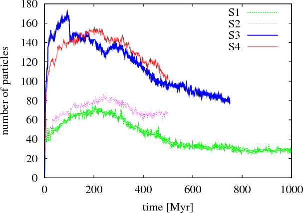 |
Figure 1: The evolution of the population of the OOC as obtained in four simulations of the OOC formation (see Sect. 2). |
| Open with DEXTER | |
In the case of the more distant outer border (cf. S3 and S4), the
stellar perturbations more support the formation than erode the OOC
during the first 100 Myr. Then, a passage of massive star
(
M* = 11.7  )
in the minimum-proximity distance from
the Sun of 434 650 AU with a time of about 94 Myr largely
depletes the OOC. The subsequent OOC population is lower when the
perturbations are considered. In the simulations S1 and S2 (less distant
outer border, 100 000 AU), the erosion of the OOC due to the
stellar perturbations prevails upon the enrichment contribution due to
the same perturbations, which lasts the whole period we are following.
)
in the minimum-proximity distance from
the Sun of 434 650 AU with a time of about 94 Myr largely
depletes the OOC. The subsequent OOC population is lower when the
perturbations are considered. In the simulations S1 and S2 (less distant
outer border, 100 000 AU), the erosion of the OOC due to the
stellar perturbations prevails upon the enrichment contribution due to
the same perturbations, which lasts the whole period we are following.
The qualitative behaviour of the OOC-population evolution is similar in all performed simulations. For S1, S2, and S4, the maximum of the population occurs at 200 to 300 Myr. For S3, an increase to this ``regular'' maximum is obviously interrupted by the above-mentioned strong stellar perturbation and the actual maximum appears earlier, at about 90-100 Myr. After the maximum, a general, relatively steep decrease can be observed till about 500 Myr (or 400 Myr in S2) in all simulations. Then, a shallower decrease is apparent in S1, which was performed for a period longer than 0.5 Gyr and is shown for 1 Gyr period. To see if this shallower decrease also occurs in the case of more distant TP outer border (400 000 AU), simulation S3 is prolonged till 0.75 Gyr and the shallower decrease is confirmed.
The influence of our choice on the outer border, up to which the TPs
are followed, can be estimated by comparing the OOC population when
longer (400 000 AU) and shorter (100 000 AU) distances of
the border are considered. In more detail, we consider the simulations
S1 and S3 with the stellar perturbations included. It appears that the
number of TPs in the region limited by the sphere of radius equal to
100 000 AU is higher about the factor of 1.75 (1.70) at 0.75 Gyr
(0.5 Gyr) in S3 with the more extended outer border than in S1 with
the closer outer border. Although this is a significant increase that
indicates that the region of the numerical integration of TP orbits
cannot be deliberately limited, it still cannot explain the difference
between our own and DLDW results. For the 400 000 AU border
(simulation S3), the OOC formation efficiency is  at
0.75 Gyr and is expected to decrease in time. DLDW obtained the
efficiency of
at
0.75 Gyr and is expected to decrease in time. DLDW obtained the
efficiency of  ,
in their ``cold run'' at 4 Gyr. In our S3
simulation, only about
,
in their ``cold run'' at 4 Gyr. In our S3
simulation, only about  TPs, the OOC residents, are situated in
the interval of heliocentric distance from 100 000 to
400 000 AU at 0.75 Gyr.
TPs, the OOC residents, are situated in
the interval of heliocentric distance from 100 000 to
400 000 AU at 0.75 Gyr.
The omission of stellar perturbations and/or the enlargement of
the region in which TPs are followed have practically no influence on
the population of inner Oort cloud (defined by
![]() AU;
AU) in our simulations,
see Leto et al. (2008).
AU;
AU) in our simulations,
see Leto et al. (2008).
3 The influence of the number of TPs in the sample
The uncertainty of the OOC-population size was not determined in Paper I. Such a determination can be done by a repeating the simulation with other sets of not identical TPs. Since the repetitions of the original simulation are much time and computational capacity consuming, we attempt to estimate at least an upper limit to the uncertainty in our S3 simulation. We divide the set of 10 038 TPs considered in this simulation into five subsets, each containing 2 008 (or 2 007) TPs. The division is made in such a way that the distributions of the initial orbital elements in each subset are the same, but the exact coordinate and velocity vectors of the TPs are not identical.
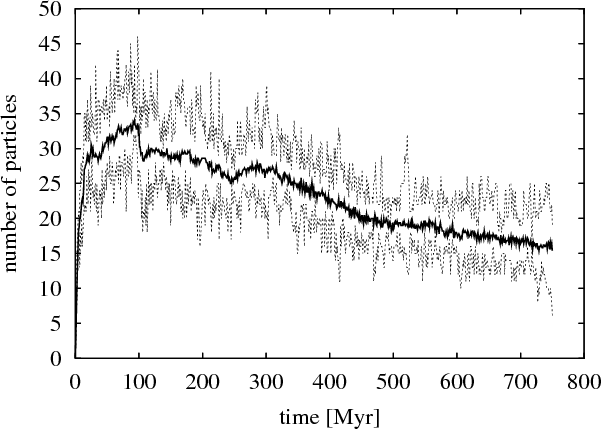 |
Figure 2: The maximum dispersion (delimited by the down and upper dotted curves) of the OOC population during its 0.75 Gyr evolution (see Sect. 3). |
| Open with DEXTER | |
The evolution of minimum and maximum numbers of TPs in the OOC, which resulted from these five subsets, are shown in Fig. 2, lower and upper dotted curves, respectively. The thick, black curve in the middle shows the evolution of the OOC population from the original, 10 038-TP, S3 simulation calibrated (divided by 5) with respect to the numbers of TPs in the subsets.
The typical (average) deviation of the subset population from the
whole-S3 population is about  .
In other words, a simulation with
a TP sample consisting of 2 000 TPs can map the evolution
of the OOC population with an uncertainty of ,
typically.
Of course, we can expect that the uncertainty in a simulation will be
lower with a larger number of TPs. The uncertainty lower than
cannot explain the difference between our own and the
DLDW formation efficiencies.
.
In other words, a simulation with
a TP sample consisting of 2 000 TPs can map the evolution
of the OOC population with an uncertainty of ,
typically.
Of course, we can expect that the uncertainty in a simulation will be
lower with a larger number of TPs. The uncertainty lower than
cannot explain the difference between our own and the
DLDW formation efficiencies.
However, the deviation can, from time to time, rise above such a high
value as  .
This is also the case of the values of OOC formation
efficiency obtained from the individual subsets for 0.75 Gyr, which
are
.
This is also the case of the values of OOC formation
efficiency obtained from the individual subsets for 0.75 Gyr, which
are  ,
,
 ,
,
,
,
 ,
and
,
and  .
The large
difference between the minimum and maximum values (
and
)
indicates a stochasticity of the OOC formation process, which
is also noticed by Kaib & Quinn (2008) in the context of minimum
stellar approach to the Sun. This stochasticity (in our own and/or DLDW
simulations), in combination with the enlargement of the TP-orbit
integration region (in our simulation), appears to be a suitable reason,
which could account for the analysed formation-efficiency difference.
.
The large
difference between the minimum and maximum values (
and
)
indicates a stochasticity of the OOC formation process, which
is also noticed by Kaib & Quinn (2008) in the context of minimum
stellar approach to the Sun. This stochasticity (in our own and/or DLDW
simulations), in combination with the enlargement of the TP-orbit
integration region (in our simulation), appears to be a suitable reason,
which could account for the analysed formation-efficiency difference.
When speaking about the stochasticity, one should mainly analyse the effect of very close stellar approaches to the Sun. Because of such an approach, the velocity vector of the Sun can be changed by the passing star, so much that the Sun starts to move along a different trajectory than the substantial part of its comet cloud. The cloud is, then, stripped (Levison et al. 2004). This effect is well known and the evident dependence of the strength of the overall stellar perturbation on its perihelion distance was clearly presented in Dybczynski (2002, see Fig. 5).
4 Summary and conclusion
Three additional simulations, in combination with the original simulation performed within our previous work, were useful to reveal that the OOC formation efficiency was noticeably underestimated in our original simulation due to too short a distance, only 100 000 AU, up to which we followed the TPs representing the comet nuclei via numerical integration. Some TPs, which temporarily occurred at larger heliocentric distance and were discarded, could obviously return into the sphere of 100 000 AU radius. Discarding them was premature.
Nevertheless, the effect of too close an outer border does not reduce
the OOC population enough to explain the discrepancy between our own
and DLDW results. Since our additional simulations were performed only
for a relatively short period of 0.5 or 0.75 Gyr, we cannot exactly
quantify this effect. However, an increase in the OOC population greater
than about a factor of 2 can scarcely be expected, in this
context.
The more comprehensive stellar perturbations can affect the size of
the OOC population most probably not more than about .
In our simulation, stellar perturbations erode the OOC population more
efficiently than support its formation. Likewise, the uncertainty of the
OOC formation within the simulation is typically only ,
which is too low a value to explain the discrepancy.
However, in agreement with Kaib & Quinn (2008) who claim that
the OOC formation process is largely stochastic, we found that the
uncertainty of the OOC-formation efficiency can rarely exceed ,
and this in combination with the short TP-orbit integration region, can
eventually explain the discrepancy or at least its major part. Namely,
when the formation efficiency at 0.75 Gyr was determined by
considering the subsets of the whole S3-simulation, the maximum value
was about a factor of 3.2 higher than the minimum value. A similar
fluctuation, with the opposite sign, could possibly occur in the DLDW
simulation.
We note that Kaib & Quinn obtained a lower formation efficiency of
the outer-Oort-cloud formation than DLDW: 1.0- (in contrast
to
by DLDW). This circumstance further alleviates the original
discrepancy between our own and the DLDW results.
(in contrast
to
by DLDW). This circumstance further alleviates the original
discrepancy between our own and the DLDW results.
In conclusion, it appears to be necessary, in future research on this topic, to follow the TPs up to a heliocentric distance exceeding 100 000 AU, to improve the model of stellar perturbations including closer stellar passages than were considered in our original simulation, and, mainly, to estimate an uncertainty of determined quantities, especially the formation efficiency of the comet cloud.
Acknowledgements
P.A.D. acknowledges the partial support of this work from Polish Ministry of Science and Higher Education (year 2008, grant No. N N203 302335). G.L. thanks PI2S2 Project managed by the Consorzio COMETA, http://www.pi2s2.it and http://www.consorzio-cometa.it for the computational resources and technical support. M.J., T.P., and L.N. thank the project ``Enabling Grids for E-sciencE II'' (http://www.eu-egee.org/) for the provided computational capacity and support in a development of the computer code, which was necessary for managing tasks on the GRID. They also acknowledge the partial support of this work by VEGA - the Slovak Grant Agency for Science (grant No. 7047).
References
- Chambers, J. E. 1999, MNRAS, 304, 793 [NASA ADS] [CrossRef] (In the text)
- Dones, L., Weissman, P. R., Levison, H. F., & Duncan, M. J. 2004, in Comets II, ed. M. C. Festou, H. U. Keller, & H. A. Weaver (Arizona: Univ. Arizona Press), 153 (In the text)
- Dones, L., Levison, H. F., Duncan, M. J., & Weissman, P. R. 2005, private communication (In the text)
- Dybczynski, P. A. 2002, A&A, 396, 283 (In the text)
- Dybczynski, P. A., Leto, G., Jakubík, M., Paulech, T., & Neslusan, L. 2008, A&A, 487, 345 (Paper I) (In the text)
- Everhart, E. 1985, in Dynamics of Comets: Their Origin and Evolution, ed. A. Carusi, & G. B. Valsecchi (Dordrecht: Reidel), 185 (In the text)
- García-Sánchez, J., Weissman, P. R., Preston, R. A., et al. 2001, A&A, 379, 634
- Kaib, N. A., & Quinn, T. 2008, Icarus, 197, 221 [NASA ADS] [CrossRef] (In the text)
- Leto, G., Jakubík, M., Paulech, T., Neslusan, L., & Dybczynski, P. A. 2008, MNRAS, 391, 1350 [NASA ADS] [CrossRef] (In the text)
- Levison, H. F., Morbidelli, A., & Dones, L. 2004, AJ, 128, 2553 [NASA ADS] [CrossRef] (In the text)
- Oort, J. H. 1950, Bull. Astron. Inst. Netherlands, 11, 91 [NASA ADS] (In the text)
All Figures
| |
Figure 1: The evolution of the population of the OOC as obtained in four simulations of the OOC formation (see Sect. 2). |
| Open with DEXTER | |
| In the text | |
| |
Figure 2: The maximum dispersion (delimited by the down and upper dotted curves) of the OOC population during its 0.75 Gyr evolution (see Sect. 3). |
| Open with DEXTER | |
| In the text | |
Copyright ESO 2009
Current usage metrics show cumulative count of Article Views (full-text article views including HTML views, PDF and ePub downloads, according to the available data) and Abstracts Views on Vision4Press platform.
Data correspond to usage on the plateform after 2015. The current usage metrics is available 48-96 hours after online publication and is updated daily on week days.
Initial download of the metrics may take a while.