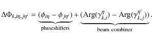
| Issue |
A&A
Volume 497, Number 3, April III 2009
|
|
|---|---|---|
| Page(s) | 963 - 971 | |
| Section | Astronomical instrumentation | |
| DOI | https://doi.org/10.1051/0004-6361/200810306 | |
| Published online | 05 March 2009 | |
An efficient phase-shifting scheme for bolometric additive interferometry
R. Charlassier - J.-Ch. Hamilton - É. Bréelle - A. Ghribi - Y. Giraud-Héraud - J. Kaplan - M. Piat - D. Prêle
APC, Université Denis Diderot-Paris 7, CNRS/IN2P3, CEA, Observatoire de Paris, 10 rue A. Domon & L. Duquet, 75205 Paris Cedex 13, France
Received 2 June 2008 / Accepted 30 January 2009
Abstract
Context. Most upcoming CMB polarization experiments will use direct imaging to search for primordial gravitational waves through the B-modes. Bolometric interferometry is an appealing alternative to direct imaging that combines the advantages of interferometry in terms of systematic effects handling and those of bolometric detectors in terms of sensitivity.
Aims. We calculate the signal from a bolometric interferometer in order to investigate its sensitivity to the Stokes parameters paying particular attention to the choice of the phase shifting scheme applied to the input channels in order to modulate the signal.
Methods. The signal is expressed as a linear combination of the Stokes parameter visibilities whose coefficients are functions of the phase shifts.
Results. We show that the signal to noise ratio on the reconstructed visibilities can be maximized provided the fact that the phase shifting scheme is chosen in a particular way called ``coherent summation of equivalent baselines''. As a result, a bolometric interferometer is competitive with an imager having the same number of horns, but only if the coherent summation of equivalent baselines is performed. We confirm our calculations using a Monte-Carlo simulation. We also discuss the impact of the uncertainties on the relative calibration between bolometers and propose a way to avoid this systematic effect.
Key words: cosmology: cosmic microwave background - techniques: interferometric - methods: data analysis
1 Introduction
Measuring precisely the polarization of the Cosmic Microwave Background (CMB) is one of the major challenges of contemporary observational cosmology. It has already led to spectacular results concerning the cosmological model (Kovac et al. 2002; Readhead et al. 2004; Dunkley et al. 2009; Nolta et al. 2009; Ade et al. 2008) describing our Universe. Even more challenging is the detection of the so-called B-modes in the CMB polarization, associated with pure tensor modes originating from primordial gravitational waves enhanced by inflation. Discovering these modes would give direct information on inflation as the amplitude of the B-modes is proportional to the tensor to scalar ratio for the amplitude of the primordial density perturbations which is a direct product of inflationary scenarii (Liddle & Lyth 2000). Furthermore, it seems that most of the inflationary models arising in the context of string theory (brane inflation, ...) predict an undetectably small scalar to tensor ratio (Kallosh & Linde 2007). The discovery of B-modes in the CMB may therefore be one of the few present ways to falsify numerous string theories. Cosmic strings and other topological defects are also sources of density perturbations of both scalar and tensor nature. They are however largely dominated by the adiabatic inflationary perturbations in TT, TE and EE power spectra and therefore are hard to detect. It is only in the B-mode sector (BB power spectrum) that the tensor topological defect perturbation could be large (Bevis et al. 2007) and have a different shape (Urrestilla et al. 2008) from those originating from inflation and hence be detectable (Pogosian & Wyman 2008).
Unfortunately, the inflationary tensor to scalar ratio seems to be rather small so that the B-modes are expected at a low level as compared to the E-modes. The quest for the B-modes is a therefore tremendous experimental challenge: one requires exquisitely sensitive detectors with an unprecedented control of the instrumental systematics, observing at a number of different frequencies to be able to remove foreground contamination. Various teams have decided to join the quest, most of them with instrumental designs based on the imager concept (BICEP Takahashi et al. 2008, EBEX Oxley et al. 2004, QUIET Samtleben et al. 2008, SPIDER Crill et al. 2008, CLOVER North et al. 2008). Another possible instrumental concept is a pairwise heterodyne interferometer that has many advantages from the point of view of systematic effects (no optics for instance) and that directly measures the Fourier modes of the sky. Let us recall that the first detections of polarization of the CMB were performed with interferometers (Kovac et al. 2002; Readhead et al. 2004). Pairwise heterodyne interferometers are however often considered as less sensitive than imagers mainly because of the additional noise induced by the amplifiers required whereas imagers use background limited bolometers. Another drawback of pairwise heterodyne interferometry is that it requires a number of correlators that scales as the square of the number of input channels, limiting the number of channels actually achievable (CMB Task Force report 2006).
A new concept of an instrument called a ``bolometric interferometer'' is currently under developement (MBI Timbie et al. 2006, BRAIN Polenta et al. 2003; Charlassier et al. 2008). In such an instrument, the interference fringes are ``imaged'' using bolometers. We believe that such an instrument could combine the advantages of interferometry in terms of systematic effects and data analysis and those of bolometers in terms of sensitivity. Sensitivity issues concerning imagers and interferometers (including bolometric) have been investigated by various authors including (Zmuidzinas 2003; Withington et al. 2008; Saklatvala et al. 2008). The goal of this article is to investigate ways to reconstruct the Fourier modes on the sky (the so-called visibilities) of the Stokes parameters with a bolometric interferometer. In particular, we focus our attention on the necessary phase shifting schemes required to modulate the fringe patterns observed with the bolometer array. We show that one can construct phase sequences that allow one to achieve an excellent sensitivity on the visibilities: scaling as
 (where
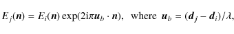
  is the number of horns and
 is the number of pairs of horns separated by identical vectors, hereafter called equivalent baselines), whereas it would scale as
 for a non optimal phase shifting sequence.
This article is organised as follows: in Sect. 2 we describe the assumptions that we make on the hardware design and on the properties of the various parts of the detector. In Sect. 3 we describe how the signal measured by such an instrument can be expressed in terms of the Stokes parameter visibilities. We show how to invert the problem in an optimal way in Sect. 4 and show how the phase shifting scheme can be chosen so that the reconstruction is indeed optimal in Sect. 5. We have validated the method we propose using a Monte-Carlo simulation described in Sect. 6. We end with some considerations about systematic effects induced by cross-calibration errors and propose a way to avoid them in Sect. 7.
![\begin{figure}
\par\includegraphics[angle=270,width=6.5cm,clip]{0306fig1.ps}
\end{figure}](/articles/aa/full_html/2009/15/aa10306-08/img15.png) |
Figure 1: Schematic view of the bolometric interferometer design considered in this article. |
| Open with DEXTER | |
2 Bolometric interferometer design
In this section we will describe the basic design we assume for the bolometric interferometer and how the incoming radiation is transmitted through all of its elements. This will lead us to a model of the signal that is actually detected at the output of the interferometer. A schematic view of the bolometric interferometer is shown in Fig. 1
2.1 Horns
We assume that we are dealing with an instrument which is observing the sky through
input horns placed on an array at positions
 .
All horns are supposed to be coplanar and looking towards the same direction on the sky. They are characterized by their beam pattern on the sky denoted
.
All horns are supposed to be coplanar and looking towards the same direction on the sky. They are characterized by their beam pattern on the sky denoted
 where
where  is the unit vector on the sphere. Two horns i and j form a baseline which we label with
![]() .
The phase difference between the electric field E reaching the two horns from the same direction
of the sky is such that:
.
The phase difference between the electric field E reaching the two horns from the same direction
of the sky is such that:
where
 is the central observing wavelength.
2.2 Equivalent baselines
It is clear that if two baselines b and b' are such that
 ,
then the phase shifts associated with the two baselines are equal, a fact that we shall extensively use in the following. All baselines b such that
,
then the phase shifts associated with the two baselines are equal, a fact that we shall extensively use in the following. All baselines b such that
 form a class of equivalent baselines associated with mode
 in visibility space. For all baselines b belonging to the same class
  ,
the phase difference between the two horns i and j is the same:
,
the phase difference between the two horns i and j is the same:
The number
 of different classes of equivalent baselines depends on the array, and the number of different baselines in an equivalence class also depends on the particular class. For instance, if we consider a square array with
 horns, there are
is
2.3 Polarization splitters
In order to be sensitive to the polarization of the incoming radiation,
we also assume that at the output of each horn there is a device which
separates the radiation into two orthogonal components denoted  and
and  .
Such a separation can be achieved with an orthomode
transducer (OMT) in wave-guide (Pisano et al. 2007), finline (Chattopadhyay et al. 1999)
or planar (Engargiola et al. 1999; Grimes et al. 2007) technologies. Each horn
therefore has two outputs measuring the electric field integrated
through the beam in the two orthogonal directions. The electric field at the output of the polarization splitter corresponding to horn i coming from direction
for polarization
.
Such a separation can be achieved with an orthomode
transducer (OMT) in wave-guide (Pisano et al. 2007), finline (Chattopadhyay et al. 1999)
or planar (Engargiola et al. 1999; Grimes et al. 2007) technologies. Each horn
therefore has two outputs measuring the electric field integrated
through the beam in the two orthogonal directions. The electric field at the output of the polarization splitter corresponding to horn i coming from direction
for polarization  (
or )
is defined by
(
or )
is defined by
 as:
as:
 |
(3) |
2.4 Phase shifters
Important components of the required setup are the phase shifters
placed on each of the outputs that allow the phase of the electric
field to be shifted by a given angle that can be chosen and controlled
externally. As will be shown later in this article, modulating the phases of the input channels is necessary to reconstruct the polarized visibilities (that can be related to cosmological information) from the signal on the detectors. For now we do not make any assumptions on the possible values of the angles but we will see that they have to be chosen carefully in order to optimize the signal to noise ratio. The signal after phase shifting coming from direction
with polarization is:
 |
(4) |
For obvious hardware reasons, all phase shifters in the setup have to be identical and deliver the same possible phase shifts.
2.5 Beam combiner
In order to be able to perform interferometry, the beam of each horn
has to be combined with all the others so that all possible baselines
are formed. The realization of a beam combiner is an issue in itself
that will not be assessed in the present article. As an example, this
can be achieved using a Butler combiner (Butler 1961,Dall'Omo 2003) or
with a quasi-optical Fizeau combiner such as the one used for
the MBI instrument (Timbie et al. 2006). All of these devices are such
that the
 input channels result after passing through the
beam combiner in
input channels result after passing through the
beam combiner in
 output channels that are linear
combinations of the input ones. To be able to conserve the input power
in an ideal lossless device, the number of output channels
has to be at least equal to the number of input channels
.
In the
output channel k, the electric field coming from direction
is
output channels that are linear
combinations of the input ones. To be able to conserve the input power
in an ideal lossless device, the number of output channels
has to be at least equal to the number of input channels
.
In the
output channel k, the electric field coming from direction
is
 :
:
 |
(5) |
where the
 coefficients model the beam combiner,
 or 0 respectively corresponds to
and polarizations. We choose to deal with configurations where the incoming
power is equally distributed among all output channels: the coefficients
or 0 respectively corresponds to
and polarizations. We choose to deal with configurations where the incoming
power is equally distributed among all output channels: the coefficients
 have unit modulus:
(one dimension is k and the other is
have unit modulus:
(one dimension is k and the other is  ).
).
In order to simplify the notation, we include the
phases in the phase shifting terms as
![]() so that:
so that:
2.6 Total power detector
The signal from each of the outputs of the combiner is not detected in a coherent way as in a pairwise heterodyne interferometer but with a bolometer through its total power averaged on time scales given by the time constant of the detector (larger than the EM wave period). The power on a given bolometer is:

The signal coming from different directions in the sky are incoherent so that their time averaged correlation vanishes:
| |
= | (9) | |
 |
(10) |
From now on, z is implicitely replaced by its time-averaged value. The signal on the bolometers is finally:
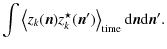
3 Stokes parameter visibilities
Developing the signal on the bolometers in terms of the incoming electric fields easily shows autocorrelation terms for each channel as well as cross-correlation terms between all the possible pairs of channels:
![$\displaystyle \left. +2{\rm Re}\left[\sum_{i<j}\sum_{\eta_1,\eta_2} \epsilon_i^...
...Phi^{\eta_1}_{k,i}-\Phi^{\eta_2}_{k,j})\right)
\right] \right\} {\rm d}\vec{n}.$](/articles/aa/full_html/2009/15/aa10306-08/img59.png)
The electric fields from different horns are related through Eq. (2) and introduce the Stokes parameters that are generally used to describe a polarized radiation:
| I | = | (13) | |
| Q | = | (14) | |
| U | = | (15) | |
| V | = | (16) |
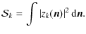
The Stokes parameter visibilities are defined as (S stands for I, Q, U or V):
 |
(17) |
The phase shift differences for a baseline b formed by horns i and j measured in the channel k are:
| (18) | |||
| (19) | |||
| (20) | |||
| (21) |
Putting all these definitions into Eq. (12) and after some calculations one finds that the signal on the bolometer k can be expressed purely in terms of the Stokes parameter visibilities and the phase shifting values (the subscript b stands for all the
 available baselines and nk is the noise):
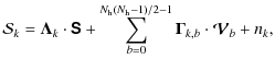
where the first term is the autocorrelations of all horns and the second one contains the cross-correlations, hence the interference patterns. We have used the following definitions:
![$\displaystyle \vec{\Gamma}_{k,b}=\frac{1}{N_{\rm out}}\left( \begin{array}{c}
\...
...}_b)\right]\\
{\rm Im}\left[{\rm {V}_V}(\vec{u}_b)\right]
\end{array} \right).$](/articles/aa/full_html/2009/15/aa10306-08/img72.png)
All of this can be regrouped as a simple linear expression involving a vector with all the sky information (Stokes parameter autocorrelations
 and all visibilities
 )
labelled
)
labelled  and another involving the phase shifting informations (
 and
and
 )
labelled
)
labelled  :
:
| (25) |
Finally, various measurements of the signal coming from the
different channels and/or from different  time samples with different phase shifting configurations can be regrouped together (the index k now goes from 0 to
 )
by adding columns to
)
by adding columns to  which then becomes a matrix A and transforming the individual measurement
 into a vector
 :
:

where A,
and
are easily expressed as a function of the quantities defined above (the total number of baselines is

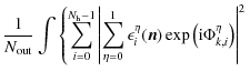
4 Reconstruction of the visibilities
Once one has recorded enough data samples to invert the above linear problem (we will call such a period a sequence in the following), the solution is the usual one assuming that the measurement noise covariance matrix is
 :
:
with covariance matrix:
4.1 Regrouping equivalent baselines
One sees that the dimension  of the
vector of unknowns is rather large:
of the
vector of unknowns is rather large:
 where
where
![]() is the number of baselines formed by the input horn array. For a large horn array this number can become very large. A
is the number of baselines formed by the input horn array. For a large horn array this number can become very large. A
 array has for instance Nb=4950 baselines and
 unknowns. One needs at least as many data samples as unknowns (and in many cases more than that) so this would involve manipulations of very large matrices. In fact as we said before, depending on the relative positions of the input horns, there may be a lot of equivalent baselines: different pairs of horns separated by the same vector
hence measuring exactly the same visibilities. It is clearly advantageous to regroup these equivalent baselines together in order to reduce the dimension of the system. As we will see below there is a huge added-advantage in doing it this way in terms of signal-to-noise ratio if one chooses the phase shifter angles wisely.
unknowns. One needs at least as many data samples as unknowns (and in many cases more than that) so this would involve manipulations of very large matrices. In fact as we said before, depending on the relative positions of the input horns, there may be a lot of equivalent baselines: different pairs of horns separated by the same vector
hence measuring exactly the same visibilities. It is clearly advantageous to regroup these equivalent baselines together in order to reduce the dimension of the system. As we will see below there is a huge added-advantage in doing it this way in terms of signal-to-noise ratio if one chooses the phase shifter angles wisely.
In the case where the input horn array is a square grid with size
 ,
the number of different classes of equivalent baselines is
,
the number of different classes of equivalent baselines is
![]() for a
horn array, hence reducing the number of unknowns to 1443 which is a very large improvement. It is obvious that all equivalent baselines measure the same visibilities and can therefore be regrouped in the linear problem leading to the same solution as considering the equivalent baselines separately. One just has to reorder the terms in Eq. (22) as first a sum over all different baselines
and then a sum over each of the baselines
for a
horn array, hence reducing the number of unknowns to 1443 which is a very large improvement. It is obvious that all equivalent baselines measure the same visibilities and can therefore be regrouped in the linear problem leading to the same solution as considering the equivalent baselines separately. One just has to reorder the terms in Eq. (22) as first a sum over all different baselines
and then a sum over each of the baselines  equivalent to
on the output line k:
equivalent to
on the output line k:
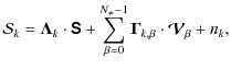
changing the
 vector to:
The global system to be solved is written in the same way as before
 ,
where the matrix A and the vectors
and
are constructed as defined in Eq. (27). Each column of the matrix A corresponds to phase shifter configurations encoded in
,
where the matrix A and the vectors
and
are constructed as defined in Eq. (27). Each column of the matrix A corresponds to phase shifter configurations encoded in
 (for all different baselines )
and
.
(for all different baselines )
and
.
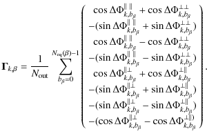
4.2 Coherent summation of equivalent baselines
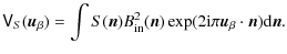
We now investigate the noise covariance matrix for the reconstructed visibilities and how one could optimize it. The noise coming from one horn illuminating one bolometer with the power P0 during one time sample is (Bowden et al. 2004; Lamarre 1986):
| (32) |
where
 is called the ``shot noise'' term and ab P02 the ``photon bunching'' term
horns illuminate
bolometers, so the total power on one bolometer is
is called the ``shot noise'' term and ab P02 the ``photon bunching'' term
horns illuminate
bolometers, so the total power on one bolometer is
 |
= | 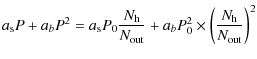 |
(33) |
 |
 |
(34) |
because
 .
We shall therefore use this upper limit to express the noise covariance matrix of the measured data samples. We assume for simplicity that the noise is stationary and uncorrelated from one data sample to another and that the combiner is lossless (for a Butler combiner this is true if
.
We shall therefore use this upper limit to express the noise covariance matrix of the measured data samples. We assume for simplicity that the noise is stationary and uncorrelated from one data sample to another and that the combiner is lossless (for a Butler combiner this is true if
 ). The noise covariance matrix is then diagonal and is written:
 |
(35) |
where
 is the
 identity matrix (
 is the number of data samples taken during
time samples with
output channel). The visibilities covariance matrix (see Eq. (29)) is written:
is the number of data samples taken during
time samples with
output channel). The visibilities covariance matrix (see Eq. (29)) is written:
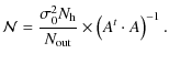 |
(36) |
We have regrouped all equivalent baselines together in A; each of its elements is therefore the sum on
sines and
cosines of the phase shifting angles (as expressed in Eq. (31)).
We will assume here that the angles are chosen randomly and uniformly
from a set of possible values between 0 and  .
Now there are
two possibilities depending on the choice of the phase shifting angles
for all baselines equivalent to a given one: they can all be different
or they can all be equal. We refer to this choice as incoherent
or coherent summation of equivalent baselines:
.
Now there are
two possibilities depending on the choice of the phase shifting angles
for all baselines equivalent to a given one: they can all be different
or they can all be equal. We refer to this choice as incoherent
or coherent summation of equivalent baselines:
- Incoherent summation of equivalent baselines: each of the
sum of the two sine/cosine functions of the uniformly distributed
angles has zero average and a variance 1. Each element of
is the sum of
of these and the Central Limit
Theorem states that it will have zero average and a variance
 .
.
- Coherent summation of equivalent baselines: then each element
of
is
 times the same angle contribution with variance 1. The matrix elements
ends up having a variance
times the same angle contribution with variance 1. The matrix elements
ends up having a variance
 .
.
 ,
the multiplication by the transpose will add all the
,
the multiplication by the transpose will add all the  different data samples. The off-diagonal elements will cancel out because the angles are uncorrelated from one channel to another. The average of the diagonal elements will be the variance of the elements in A multiplied by .
So finally, depending on the choice between incoherent or coherent summation of equivalent baselines, the visibility covariance matrix will scale in a different manner:
different data samples. The off-diagonal elements will cancel out because the angles are uncorrelated from one channel to another. The average of the diagonal elements will be the variance of the elements in A multiplied by .
So finally, depending on the choice between incoherent or coherent summation of equivalent baselines, the visibility covariance matrix will scale in a different manner:
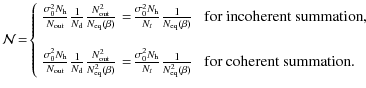
Of course the evaluation above is only valid in a statistical sense, insofar as the phase shifts are really randomly chosen. If this the case, Eq. (37) are true up to random corrections of relative order
 .
The latter scaling in Eq. (37) is clearly more advantageous and optimises the reconstruction of the visibilities. In fact this result is quite obvious: if the phase shifting angles for equivalent baselines are all different,
the coefficients of the linear problem that one wants to invert will always be smaller than if the summation of equivalent baselines is performed coherently. The signal to noise ratio on the visibilities will therefore be optimal if one maximises the coefficients, which is obtained by choosing the coherent summation.
.
The latter scaling in Eq. (37) is clearly more advantageous and optimises the reconstruction of the visibilities. In fact this result is quite obvious: if the phase shifting angles for equivalent baselines are all different,
the coefficients of the linear problem that one wants to invert will always be smaller than if the summation of equivalent baselines is performed coherently. The signal to noise ratio on the visibilities will therefore be optimal if one maximises the coefficients, which is obtained by choosing the coherent summation.
4.3 Comparison with classical interferometers and imagers
The variance on the visibilities obtained above in the case of a coherent summation of equivalent baselines can be rewritten:
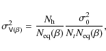 |
(38) |
that can be compared
 .
We see that the only difference introduced by bolometric interferometry is the factor
.
We see that the only difference introduced by bolometric interferometry is the factor
 .
On average, the number of equivalent baselines is
.
On average, the number of equivalent baselines is
 closer to one. The resulting expression of the variance on visibilities for bolometric interferometry therefore only differs by this slightly larger than one factor with respect to pairwise heterodyne interferometry. The important point is that the value of
  for bolometric interferometry is typical of a bolometer (photon noise dominated) hence smaller than what can be achieved with HEMT amplifiers in a pairwise heterodyne interferometer.
This result can be summarized as follows: a bolometric interferometer using coherent summation of equivalent baselines can achieve the sensitivity that would be obtained with a pairwise heterodyne interferometer with the noise of a bolometric instrument (and without the complexity issues related to the large number of channels). Such an instrument would therefore also be competitive with an imager that would have the same number of bolometers as we have input channels in our bolometric interferometer. This is shown in Hamilton et al. (2008)
where a detailed study comparing a bolometric interferometer, a pairwise heterodyne interferometer and an imager from the sensitivity point of view is done. On the other hand, if the equivalent baselines are summed incoherently, it is obvious that the sensitivity would be very poor due to the absence of the
 additional factor. However, bandwidth is usually an additionnal difficulty in interferometry, limiting the sensitivity at small scales as signals at different frequencies do not interfere coherently. The problem of bandwidth is now under detailed study.
The next section shows how it is possible to choose the phase shifting sequences in such a way that the prescription of coherent summation of equivalent baselines is enforced.
5 Choice of the optimal phase sequences
One wants the phase shifting scheme to be such that equivalent baselines have exactly the same sequence but that different baselines have different phase shifts so that they can be disentangled by the linear inversion corresponding to Eq. (30). Now let's see how to comply with this constraint of having equivalent baselines correspond to identical phase differences. As can be seen in Eq. (6), the phase shifts have two different origins: the phase shifters themselves whose angles can be chosen to follow a given sequence and are the same for all output channels and the phase shifts coming from the beam combiner. Each input is labelled by the horn number
 and the polarization direction .
Each output is labelled by its number
and the polarization direction .
Each output is labelled by its number
 .
The phase shift differences are therefore
.
The phase shift differences are therefore
 |
(39) |
![\begin{figure}
\par\includegraphics[angle=-90,width=7cm,clip]{0306fig2.ps}
\end{figure}](/articles/aa/full_html/2009/15/aa10306-08/img141.png) |
Figure 2: Choosing all the phase sequences from that of one horn and two phase sequence differences (represented in green). |
| Open with DEXTER | |
a) Phase shifter phase differences (unpolarized case):
We assume that the horns are placed on a square array with size
as in Fig. 2. In this case, the position of all horns canbe parametrized, in units of the minimum horn separation, as a
vector
 where li and mi are integers running from 0 to
 such that
 .
In this case, we have seen that there are
.
In this case, we have seen that there are
![]() different classes of equivalent baselines labelled
.
Forgetting about polarization, the phase sequences can be constructed from a vector of two independent random phase sequences h(t) and v(t) which separate the horizontal
and vertical directions in the horn array:
different classes of equivalent baselines labelled
.
Forgetting about polarization, the phase sequences can be constructed from a vector of two independent random phase sequences h(t) and v(t) which separate the horizontal
and vertical directions in the horn array:
The phase shift difference associated with the baseline between horns i and j is
and it is clear that the phase shift difference sequences will be the same for all baselines such that
 ,
where
is one of the classes of equivalent baselines. Because the two random sequences h(t) and v(t) have been chosen independently, the phase sequences associated with two different baseline classes
,
where
is one of the classes of equivalent baselines. Because the two random sequences h(t) and v(t) have been chosen independently, the phase sequences associated with two different baseline classes
 will be different.
b) Separating polarizations:
Looking at formula (24), it is clear that one will not
be able to separate  and
and  visibilities, unless one uses two independent vectors of sequences
 .
However, in this case
.
However, in this case  and
and  are not measured with maximum
accuracy because the phase shift differences
are not measured with maximum
accuracy because the phase shift differences
are not equal for two different but equivalent baselines, so that they do not add coherently. One is therefore led to use alternately two measuring modes:
- 1.
- One mode where
,
where phase shifts differences read:
In this mode,
and
are measured with maximum accuracy (noise reduction
 ), but
and
are only measured with noise a reduction
), but
and
are only measured with noise a reduction
 .
.
- 2.
- One mode with
 .
Then
however, one cannot measure
because
.
Then
however, one cannot measure
because
therefore one must introduce two more sequences (one of them may be zero) independent from one another and from
 ,
such that
,
such that
 .
Then:
.
Then:
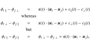
which means that,
and
are measured with maximum accuracy (noise reduction
), but
is not measured at all.
 phase shifts
(let us call this ensemble
phase shifts
(let us call this ensemble  )
but in different order. If
)
but in different order. If
 ,
,
 and
and
 are sequences of elements belonging
to ,
then the phase for any horn also has to belong to ,
meaning that
.
As shown in Appendix A, this
requires us to choose the
values of the phase shifts regularly
spaced between 0 and as:
are sequences of elements belonging
to ,
then the phase for any horn also has to belong to ,
meaning that
.
As shown in Appendix A, this
requires us to choose the
values of the phase shifts regularly
spaced between 0 and as:
 |
(42) |
The elementary sequences
,
and
are uniform random samples of  values taken among the elements of .
They must be chosen independent from one another
to make sure that unequivalent baselines do not share the same sequence
of phase differences.
values taken among the elements of .
They must be chosen independent from one another
to make sure that unequivalent baselines do not share the same sequence
of phase differences.
c) Beam combiner phase difference:
As was said before there are two main designs for the beam combiner: Butler combiner (Dall'Omo 2003) or quasi optical combiner (Timbie et al. 2006). Without going into details, let us say that identical phase shifts for equivalent baselines are naturally obtained for the quasi optical combiner, and are achieved through an adequate wiring for the Butler combiner.
d) Summary and expected accuracy:
Finally, in order to recover the visibilities keeping to the ``coherent
summation of equivalent baselines'' criterion, one has to build
phase sequences that successively follow modes 1 and 2 on an equal
footing, build the corresponding A matrix and solve the system.
There is a price to pay: during the first half sequence,
and
are measured with optimal accuracly but
and
are
not, during the second half sequence, ,
 and
are
measured with optimal accuracy but
is not measured at all.
We therefore expect the sensitivity on ,
and to decrease by roughly a factor of
and
are
measured with optimal accuracy but
is not measured at all.
We therefore expect the sensitivity on ,
and to decrease by roughly a factor of  with respect to the
sensitivity on ,
although the sensitivity on
and will be slightly better constrained than on .
with respect to the
sensitivity on ,
although the sensitivity on
and will be slightly better constrained than on .
6 Monte-Carlo simulations
![\begin{figure}
\par\includegraphics[width=8cm,angle=0,clip]{0306fig3.ps}\includegraphics[width=8cm,angle=0,clip]{0306fig4.ps}
\end{figure}](/articles/aa/full_html/2009/15/aa10306-08/img175.png) |
Figure 3:
Relative rms on visibility residuals for |
| Open with DEXTER | |
 scaling for each strategy to exhibit only the dependence with the number of equivalent baselines. The data points were fitted with linear slopes io
  -
- than the other strategies that both scale as
 .
.We have investigated what was discussed above using Monte-Carlo simulations. There are three approaches that have to becompared for the reconstruction of the Stokes parameter visibilities:
- considering all baselines independantely without regrouping the equivalent ones. We expect this method to have error bars scaling as
 .
The system to solve is large in that case;
.
The system to solve is large in that case;
- regrouping the equivalent baselines without any choice of the phase shifts so that they do not add in a coherent way. We expect this method to be exactly equivalent to the previous one but with a reduced size of the matrices;
- following the strategy to regroup equivalent baselines and choosing the phases so that they are coherently added. We expect the error bars to scale as
and therefore be the most efficient.
,
and
a hundred times lower than
as expected from the CMB and calculated the signal expected on the bolometers using the phase shift values for the three above strategies. We then added Gaussian noise with a variance
 to the bolometer signal. In each case we have performed a large number of noise and phase shift sequence realisations. For each realisation, we have stored the reconstructed and input visibilities and analysed the residual distributions. We have investigated the three above strategies and also the behaviour of the third one (coherent summation of equivalent baselines) with respect to the two free parameters: the length of the phase shift sequence before inverting the linear problem and the number of different phase shift angles (regularly spaced between 0 and
as shown in Appendix A).
to the bolometer signal. In each case we have performed a large number of noise and phase shift sequence realisations. For each realisation, we have stored the reconstructed and input visibilities and analysed the residual distributions. We have investigated the three above strategies and also the behaviour of the third one (coherent summation of equivalent baselines) with respect to the two free parameters: the length of the phase shift sequence before inverting the linear problem and the number of different phase shift angles (regularly spaced between 0 and
as shown in Appendix A).
6.1 Scaling with the number of equivalent baselines
We show in Fig. 3 the scaling of the rms residuals on the visibilities as a function of the number of equivalent baselines. We have divided the rms by
 in order to isolate the effects that are specific to bolometric interferometry and depend on the way equivalent baselines are summed (see Eq. (37)). We see that as expected the scaling is
  if one solves the problem by maximizing the signal to noise ratio using our coherent summation of equivalent baselines. The poor
scaling is also observed when all baselines are considered separately or when the phase shift angles are not chosen optimally.
if one solves the problem by maximizing the signal to noise ratio using our coherent summation of equivalent baselines. The poor
scaling is also observed when all baselines are considered separately or when the phase shift angles are not chosen optimally.
6.2 Scaling with the number of samples and number of different phases
![\begin{figure}
\par\includegraphics[width=8cm,clip]{0306fig5.ps}\includegraphics[width=8cm,angle=0]{0306fig6.ps}
\par\end{figure}](/articles/aa/full_html/2009/15/aa10306-08/img181.png) |
Figure 4:
Scaling of the rms residuals (divided by
|
| Open with DEXTER | |
 )
on the Stokes parameter visibilities with respect to the number of different phases achieved by the phase shifters and the number of different phase configurations used for the analysis (length of the sequence). One sees on the left that for a number of horns of 64 one needs at least 12 or 13 different angles to be able to solve the linear problem. It is clear from the plot on the right that the longer the sequence, the better the residuals, but a plateau is rapidly reached when the number of samples is around 4 times the number of unknowns in the linear problem. One can also see the factor
)
on the Stokes parameter visibilities with respect to the number of different phases achieved by the phase shifters and the number of different phase configurations used for the analysis (length of the sequence). One sees on the left that for a number of horns of 64 one needs at least 12 or 13 different angles to be able to solve the linear problem. It is clear from the plot on the right that the longer the sequence, the better the residuals, but a plateau is rapidly reached when the number of samples is around 4 times the number of unknowns in the linear problem. One can also see the factor
 between the accuracy on the intensity and the polarized Stokes parameters due to the two-step phase shifting scheme that we have to perform to be able to reconstruct them all.
Let's now concentrate on the optimized strategy described above: coherent summation of equivalent baselines. We show in Fig. 4 the scaling of the rms residuals on the visibilities with respect to the length of the sequence and the number of different phases achieved by the phase shifters (as shown in Appendix A, these have to be regularly spaced between 0 and ). The rms values have been divided by

One observes (Fig. 4 left) that the linear problem is singular when the number of different phases is not sufficient. Varying the number of horns in the array led us to derive the general scaling 
 for the minimum number of phases. Increasing the number of possible angles does not improve the residuals. Concerning the length of the sequence (Fig. 4 right), one observes that when it is slightly larger than the number of unknows (
 where
is the number of different baselines,
where
is the number of different baselines,
![]() for a square array) then the reconstruction of the visibilities is not optimal due to the lack of constraints. Optimality is progressively reached when integrating a larger number of samples before inverting the problem. A reasonable result is obtained when
for a square array) then the reconstruction of the visibilities is not optimal due to the lack of constraints. Optimality is progressively reached when integrating a larger number of samples before inverting the problem. A reasonable result is obtained when
 .
The expected
difference between the accuracy on
and that on ,
and
(due to the fact that we have have to perform two successive phase shifting schemes in order to measure all three polarized visibilities) is also confirmed by the simulation.
.
The expected
difference between the accuracy on
and that on ,
and
(due to the fact that we have have to perform two successive phase shifting schemes in order to measure all three polarized visibilities) is also confirmed by the simulation.
7 How to proceed with a realistic instrument?
When dealing with a realistic instrument one has to account for systematic errors and uncertainty to choose the precise data analysis strategy. We do not want to address the broad topic of systematic effects with bolometric interferometry in this article (we refer the interested reader to (Bunn 2007) where systematic issues for interferometry are treated in a general way) but stress one point that is specific to the method we propose here, related to intercalibration of the bolometers in the detector array.
Inverting the linear problem in Eq. (30) is expressing the Stokes parameter visibilities as linear combinations of the
signal measurements performed with different phase shifting configurations. These measurements can be those of the
bolometers each in
time samples. This is where intercalibration issues have to be considered. Linear combinations of signals measured by different bolometers are extremely sensitive to errors in intercalibration and will induce leakage of intensity into the polarized Stokes parameters if it is not controlled with exquisite accuracy. So we claim that combining different bolometers in the reconstruction of the visibilities in a bolometric interferometer such as the one we describe here is not a wise choice unless the bolometer array is very well intercalibrated (through precise flat-fielding). The solution we propose is to treat all the bolometers independantly, inverting the linear problem separately for each of them. This requires many time samples for the phase shift sequences but is safer from the point of view of systematics. As a realistic example, for a
elements square input array, the number of different baselines is 180 and the number of unknowns is 1443. An optimal reconstruction of the visibilities can therefore be achieved with  6000 time samples. The duration of the time samples is driven by both the time constant of the bolometers (very short with TES) and the speed achieved by the phase shifter to switch from one phase to the other. A reasonable duration for the time samples is about 10 ms which would correspond to sequences lasting about one minute. It is likely that the cryogenic system of such a bolometric interferometer would ensure a stable bath on the minute time scale so that the knee frequency of the bolometric signal would be smaller than 1 min-1. In such a case, the noise can be considered as white (diagonal covariance matrix) during each sequence and the inversion is easily tractable even with 6000 samples vectors. We are currently performing fully realistic simulations including systematic effects; the results will be presented in a future publication.
Conclusions
We have investigated ways to reconstruct the Stokes parameter visibilities from a bolometric interferometer. It turns out that all three complex Stokes parameter visibilities can be reconstructed with an accuracy that scales as the inverse of the number of equivalent baselines if one follows a simple prescription: all equivalent baselines have to be factorized together in a coherent way, meaning that the phase shift differences have to be equal for equivalent baselines. We have proposed a simple way to construct such phase shift sequences and tested it on a Monte-Carlo simulation. The simulation confirms that the scaling of the errors on the visibilities is
 if one follows our prescription but
otherwise.
if one follows our prescription but
otherwise.
The main conclusion of this article is therefore that a bolometric interferometer can achieve a good sensitivity only with an appropriate choice of the phase shift sequences (coherent summation of equivalent baselines). A detailed study of the sensitivity of a bolometric interferometer (Hamilton et al. 2008) shows that they are competitive with imagers and pairwise heterodyne interferometers.
We also discussed the data analysis strategy and proposed a solution for the possible cross-calibration issues between the different bolometers. Even though one has simultaneously
measurements of the signal with different phase configurations, it might be preferable not to combine these measurements but rather to reconstruct the visibilities on each bolometer separately and combine the visibilities afterwards. Such a strategy would increase the length of the phase shifting sequences, but in a reasonable (and tractable) way thanks to the intrinsic shortness of our proposed phase shifting scheme.
Acknowledgements
The authors are grateful to the whole BRAIN collaboration for fruitful discussions.
Appendix A: Proof of the necessity of having regularly spaced phase shift values
When we use the phase shift configurations of Eq. (40), the antenna with coordinates (i,j) will be phase shifted by:
 |
(A.1) |
In practice we are only able to construct a limited number of different phase shifters, and the phase shift sequences h(t), v(t) and c(t) will be independent random sequences of phase shifts taken from the same set
 of n phase shifts
  .
For all phase shifts in Eq. (A.1) to belong to ,
it is necessary that
.
For all phase shifts in Eq. (A.1) to belong to ,
it is necessary that
 (modulo )
also belongs to .
Let us write the smallest non-zero element of as:
(modulo )
also belongs to .
Let us write the smallest non-zero element of as:
 |
(A.2) |
 (modulo )
should also belong to ,
but
(modulo )
should also belong to ,
but
 |
(A.3) |
Therefore
), and cannot belong to
unless
 .
One concludes that the set
.
One concludes that the set  of n phase shifts has to be of the form:
 |
(A.4) |
which finally is a quite obvious choice.
References
- Ade, P., Bock, J., Bowden, M., et al. 2008, ApJ, 674, 22 [NASA ADS] [CrossRef] (In the text)
- Bevis, N., Hindmarsh, M., Kunz, M., et al. 2007, Phys. Rev. D, 76, 1722 [CrossRef] (In the text)
- Bock, J., Church, S., Devlin, M., et al., CMB Task Force report 2006 [arXiv:astro-ph/0604101] (In the text)
- Bunn, E. F. 2007, Phys. Rev. D, 75, 3084 [CrossRef] (In the text)
- Bowden, M., Taylor, A. N., Ganga, K. M., et al. 2004, MNRAS, 349, 321 [NASA ADS] [CrossRef] (In the text)
- Butler, J., & Lowe, R. 1961, Electron. Des. 9, 170 (In the text)
- Charlassier, R., for the BRAIN Collaboration 2008 [arXiv:0805.4527v1] (In the text)
- Chattopadhyay, G., & Carlstrom, J. E. 1999, IEEE Microwave and Guided wave letters, 9(9) (In the text)
- Crill, B., Ade, P. A. R., Battistelli, E. S., et al. 2008, Proc. SPIE, 7010[arXiv:0807.1548] (In the text)
- Dall'Omo, Ch. 2003, Ph.D. Thesis, Université de Limoges, France (In the text)
- Dunkley, J., Komatsu, E., Nolta, M. R., et al. 2009, ApJS, 180, 306 [NASA ADS] [CrossRef] (In the text)
- Engargiola, G., & Plambeck, R. L. 2003, Rev. Sci. Inst., 74, 1380 [NASA ADS] [CrossRef] (In the text)
- Grimes, P. K., King, O. G., Yassin, G., & Jones, M. E. 2007, Electronics Letters, 43, 1146 [CrossRef] (In the text)
- Hamilton, J.-Ch., Charlassier, R., Cressiot, C., et al. 2008, A&A, 491, 923 [NASA ADS] [CrossRef] [EDP Sciences] (In the text)
- Hobson, M. P., & Magueijo, J. 1996, MNRAS, 283, 1133 [NASA ADS]
- Kallosh, R., & Linde, A. 2007, JCAP, 04, 017 [NASA ADS] (In the text)
- Kovac, J., Leitch, E. M., Pryke, C., et al. 2002, Nature, 420 772 (In the text)
- Lamarre, J.-M. 1986, Appl. Opt., 25, 870 [NASA ADS] [CrossRef] (In the text)
- Liddle, A. R., & Lyth, D. H., 2000, Cosmological Inflation and Large-Scale Structure (Cambridge University Press) (In the text)
- Nolta, M. R., Dunkley, J., Hill, R. S., et al. 2009, ApJS, 180, 296 [NASA ADS] [CrossRef] (In the text)
- North, C. E., Johnson, B. R., Ade, P. A. R., et al. 2008, Proc. Rencontres Moriond[arXiv:0805.3690] (In the text)
- Oxley, P., Ade, P., Baccigalupi, C., et al. 2004, Proc. SPIE Int. Soc. Opt. Eng., 5543, 320 [NASA ADS] (In the text)
- Polenta, G., Ade, P. A. R., Bartlett, J., et al. 2007, New Ast. Rev., 51, 256 [NASA ADS] [CrossRef]
- Pogosian, L., & Wyman, M. 2008, Phys. Rev. D, 77, 083509 [NASA ADS] [CrossRef] (In the text)
- Pisano, G., Pietranera, L., Isaak, K., et al. 2007, IEEE Microwave and wireless components letters, 17, 286 [CrossRef] (In the text)
- Readhead, A. C. S., Myers, S. T., Pearson, T. J., et al. 2004, Science, 306, 836 [NASA ADS] [CrossRef] (In the text)
- Samtleben, D., et al. 2008, Proc. Renc. Moriond [arXiv:0806.4334] (In the text)
- Saklatavala, G., Withington, S., Hobson, M. P., et al. 2008, J. Opt. Soc. Am. A, 25(4), 958 (In the text)
- Takahashi, Y. D., Barkats, D., Battle, J. O., et al. 2008, Proc. SPIE, 7020, 70201 (In the text)
- Timbie, P. T., Tucker, G. S., Ade, P. A. R., et al. 2006, New Astron. Rev., 50, 999 [NASA ADS] [CrossRef] (In the text)
- Urrestilla, J., Mukherjee, P., Liddle, A. R., et al. 2008, Phys. Rev. D, 77, 123005 [NASA ADS] [CrossRef] (In the text)
- Withington, S., Hobson, M. P., & Campbell, E. S. 2008, J. Opt. Soc. Am. A, 21, 1988 [NASA ADS] (In the text)
- Zmuidzinas, J. 2003, J. Opt. Soc. Am. A, 20, 218 [NASA ADS] [CrossRef] (In the text)
Footnotes
- ... with
![[*]](/icons/foot_motif.png)
- In units of the smallest baseline in the array.
- ... term
- At 90 GHz with 30% bandwidth, the second term is not negligible if one observes from the ground. From space however, still at 90 GHz, the second term becomes negligible as the input power is significantly reduced.
- ... compared
- The notations are different:
 in (Hobson & Magueijo 1996) has to be replaced by our ;
their
in (Hobson & Magueijo 1996) has to be replaced by our ;
their
 is the number of equivalent baselines
.
In our paper
corresponds to
is the number of equivalent baselines
.
In our paper
corresponds to
 in their article as a noise equivalent power
  has to be replaced by
 when treating noise in temperature units rather than in power units.
All Figures
| |
Figure 1: Schematic view of the bolometric interferometer design considered in this article. |
| Open with DEXTER | |
| In the text | |
| |
Figure 2: Choosing all the phase sequences from that of one horn and two phase sequence differences (represented in green). |
| Open with DEXTER | |
| In the text | |
| |
Figure 3:
Relative rms on visibility residuals for |
| Open with DEXTER | |
| In the text | |
| |
Figure 4:
Scaling of the rms residuals (divided by
|
| Open with DEXTER | |
| In the text | |
Copyright ESO 2009
Current usage metrics show cumulative count of Article Views (full-text article views including HTML views, PDF and ePub downloads, according to the available data) and Abstracts Views on Vision4Press platform.
Data correspond to usage on the plateform after 2015. The current usage metrics is available 48-96 hours after online publication and is updated daily on week days.
Initial download of the metrics may take a while.