| Issue |
A&A
Volume 497, Number 2, April II 2009
|
|
|---|---|---|
| Page(s) | 583 - 587 | |
| Section | Planets and planetary systems | |
| DOI | https://doi.org/10.1051/0004-6361/200811198 | |
| Published online | 24 February 2009 | |
Additional planets in the habitable zone of Gliese 581?
R. Zollinger1 - J. C. Armstrong2
1 - Department of Physics, University of Utah, Salt Lake City, UT, 84112-0830, USA
2 -
Department of Physics, Weber State University, Ogden, UT, 84408-2508, USA
Received 21 October 2008 / Accepted 30 January 2009
Abstract
Context. The 3-planet system that contains two super Earths has recently been verified around the M dwarf Gliese 581. Recent theoretical work into the system's habitable zone (HZ) still raises questions as to the habitability of the known planets; however, the system remains the best candidate for potentially habitable planets.
Aims. We address the possible existence of an undetected, lower mass planet inside the conservative HZ through the dynamical stability evolution of the system. This is important since recent studies consider planets c and d to be at the edges of the HZ, while the region in between might harbor a better candidate for habitability. These planets have a radial velocity contribution just below the measurement uncertainty, which would be the reason they have not been detected previously. Thus, our considered planetary masses are maximum masses for the undetected planet.
Methods. Using reported planetary parameters of the three detected planets, we numerically integrate the system for 106 yr with mass-less test particles scattered inside the HZ. This specifies possible regions for stable orbits. We then integrate the system for 107 yr with a fourth lower mass planet inside the specified stability regions.
Results. Our study found a high probability that stable systems occurred for a fourth planet of 
 with a semi-major axis between 0.11 AU and 0.21 AU and eccentricity between 0.01 and 0.25. In stable systems, the fourth planet had very little effect on the overall stability of the system. There, the dynamical evolution of the three detected planets was comparable to that of 3-planet models. The eccentricity of the undetected planet had small amplitude variations and its semi axis remained extremely stable. Thus, Gliese 581 remains a good candidate for future detection of habitable Earth-mass planets.
Key words: planetary systems - stars: individual: Gliese 581 - methods: N-body simulations
1 Introduction
Recent years have seen a significant increase in extrasolar planetary detection through the radial velocity technique (Butler et al. 2006). Most detected objects are giant (Jupiter-like) planets, due to the bias of observational techniques for detecting the largest and most massive planets. Recently, higher precision has led to the discovery of planets with a minimum mass below
 .
The first one was GJ 876d, with minimum mass of
.
The first one was GJ 876d, with minimum mass of
 (Rivera et al. 2005). Planets with minimal mass between one and ten
 are often referred to as super-Earths. Super-Earths are considered rocky planets with similar chemical and mineral composition as the Earth (Valencia et al. 2007).
The M dwarf Gliese 581 is host to two super-Earths in its recently identified 3-planet system. Two years after Bonfils et al. (2005) detected a Neptune-mass object (planet b) orbiting the star, Udry et al. (2007) announced the discovery of two additional super-Earths (planets c and d). The properties of this planetary system are given in Table 1. With the announcement of the two detections, Udry et al. (2007) pointed out that the planets may lie within the habitable zone (HZ) of the star. Attempts to define the HZ of Gliese 581 and the possible habitability of the two outer planets have been subjects of recent investigation (von Bloh et al. 2007; Selsis et al. 2007; Chylek et al. (2007)). According to Selsis et al. (2007), planets Gl 581c and Gl 581d are just outside the edges of what can be considered as the conservative HZ; however, the habitability of the planets is not entirely ruled out due to uncertainties in the precise location of the HZ boundaries.
The dynamical evolution of the Gliese 581 planetary system has been previously considered by Beust et al. (2008). Their numerical integrations included various orbital inclinations, since the actual value of the inclinations are unknown. After considering various possible configurations, they concluded that the system is almost always stable. From that, they consider a 3-planet model to be a physically adequate description of the radial velocity measurements. Due to the inherent uncertainty in these measurements, the system may harbor additional, undetected planets. In the same study, Beust et al. (2008) also considered the presence of larger outer planets at the upper detection limit of the measurements. This limit placed constraints on the mass and distance of any unseen outer planet. In all the considered cases, they found that an additional outer planet had no effect on the stability of the system.
Since the search for habitable earth-like planets is a subject of recent interest, we raise the question as to the possible existence of additional undetected planets inside the 3-planet system. In this paper, we numerically investigate this possibility through the dynamical stability of the system with a fourth planet, provided the contribution of the unseen planet to the radial velocity signal is just below the actual measurement uncertainty. In particular, we confine our study to the area between Gl 581c and Gl 581d, which is considered to be inside the conservative HZ (Selsis et al. 2007). Our paper is organized as follows. In Sect. 2 we provide a brief description of the methods used in our integrations. We perform our integrations in Sect. 3, beginning with a 3-planet model that includes several test particles. We then investigate the perturbing effects of potentially undetected planets. The implications of our study are discussed in Sect. 4.
2 Methods and model parameters
To perform our computations we used the 3D hybrid symplectic integrator Mercury (Chambers 1999), which permits close encounters between massive bodies. The initial timestep was set to 0.027 day, i.e. 1/200 of the smallest orbital period. This small timestep ensures good resolution of the shortest orbit. The systems were numerically integrated over a minimum of 106 yr, during which, the fractional errors in the total energy and total angular momentum were recorded. In all cases, the energy was conserved to 10-9 relative accuracy and the angular momentum to 10-11 relative accuracy, which provides confidence in our results.
For the Gliese 581 system, we used the semi-major axis, eccentricity, and mass values listed in Table 1. Since the planets were detected using the radial velocity technique, the reported mass values are actually
 ,
where
,
where  is the planetary mass and i is the orbital inclination. Since the orbital inclinations are unknown, we made the assumptions of coplanarity and
 (i = 90 degrees, an edge-on system). All planets began integrations at perihelion.
The system was integrated in two steps. The first included test particles of negligible mass and the second involved an additional earth-like planet. In both steps, any additional bodies other than the three known planets were inserted between Gl 581c and Gl 581d (the conservative HZ). We would expect our results to vary for different inclination values, since the planetary masses would be augmented by a factor of  .
For example, an inclination of 30 degrees would double the detected masses.
.
For example, an inclination of 30 degrees would double the detected masses.
For this study, the mutual inclinations of the planets were held at 90 degrees. Further considerations at various system inclinations would significantly increase the total number of integrations. Because of the considerable time requirements, we will confine our current study to the limiting case of i = 90, plus one additional inclination of i = 45 degrees, and recognize the possibility for future research.
3 Testing for stability
3.1 Orbital stability with test particles
We integrated the 3-planet system with test particles of zero mass that were only perturbed by the massive planets. The test particles had initial parameters ranging from 0.07 AU to 0.3 AU for their semi-major axes and 0.02 to 0.2 for their eccentricities. To stay consistent with the 2-dimensional planet configurations, there is zero inclination dispersion among the particles. There were roughly one thousand test particles in total. The integrations were carried out over 106 yr.
These integrations served two purposes. The first was to ensure the stability of the 3-planet model, as was verified in the nominal case of Beust et al. (2008). This was possible since the mass-less test particles had no perturbing affect on any of the planets. The maximum evolution ranges of the planets are listed in Table 2. The semi-major axes were extremely stable while the evolution ranges of the eccentricities are narrow. Considering the short orbital periods of the planets, we have confidence that our configuration of the 3-planet model is stable.
Table 1:
Orbital parameters of the Gl 581 planetary system, from Udry et al. (2007).
 ,
where i is the orbital inclination.
,
where i is the orbital inclination.
Table 2: Variation ranges for some orbital parameters over the 106 yr integration.
The second purpose of the test particles was to isolate possible regions of orbital stability within the HZ before introducing a fourth planet into the system. As the integrations progressed, the total number of particles decreased to a steady value as they settled into stable orbits. Almost all the lost particles were cleared out during the first quarter of the integration; about half the particles remained at the end. The initial and final distributions of the test particles are represented in Fig. 1. The marked boxes show the parameter spaces for particles that maintained orbital stability throughout the integration. Well refer to the narrow box as region A, which encloses 0.08 AU < a < 0.10 AU and 0.01 < e < 0.22. The wider box is region B, which covers 0.11 AU < a < 0.21 AU and 0.01 < e < 0.25. Similar to the planets, in these regions the semi-major axes were extremely stable and the eccentricity variations were narrow.
![\begin{figure}
\par\includegraphics[width=9cm,clip]{1198f1tp.eps}\vspace*{3mm}
\includegraphics[width=9cm,clip]{1198f1bm.eps}
\end{figure}](/articles/aa/full_html/2009/14/aa11198-08/img17.png) |
Figure 1: Top: initial distribution of test particles. Bottom: final distribution at the end of the 106 yr integration. The two rectangular boxes mark the particles that maintained orbital stability throughout the integration. Box on the left is referred to as region A and the box on the right is region B. |
| Open with DEXTER | |
In Fig. 1 we also see a smaller stability cluster in the region with 0.27 AU < a < 0.3 and 0.15 < e < 0.22. Because this region lies outside our considered HZ, it was not included in the extended analysis of the parameter space.
Since the minimum masses (i = 90 degrees) were used for the three known planets, we performed additional integrations to verify that a lower inclination doesn't significantly change the stable regions. The same integrations involving test particles were repeated for an inclination of 45 degrees. The behavior of the test particles was very similar to edge-on system. The final distribution is shown in Fig. 2. Comparison of Figs. 1 and 2 shows that the particle distribution is nearly identical in the two cases.
![\begin{figure}
\par\includegraphics[width=9cm,clip]{1198fig2.eps}
\end{figure}](/articles/aa/full_html/2009/14/aa11198-08/img18.png) |
Figure 2: Final distribution of test particles for an inclined system of 45 degrees. |
| Open with DEXTER | |
3.2 Orbital stability with test planets
The aim of our study is to test the likelihood of undetected planets within the conservative HZ. The previous section helped define the regions of possible orbital stability for objects with sufficiently low mass. To remain undetected, the unseen planet should not generate a radial velocity with larger amplitude than the measurement uncertainty. This limits the possible mass m and semi-major axis a of the unseen planet. Assuming an inclination of 90 degrees, we derive
 |
(1) |
where
 is the observed radial velocity and M* is the stellar mass. Given a radial velocity of
 ,
which is comparable to the uncertainty referenced by Udry et al. (2007), Eq. (1) becomes
,
which is comparable to the uncertainty referenced by Udry et al. (2007), Eq. (1) becomes
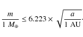 |
(2) |
Equation (2) corresponds to the maximum possible mass for a planet to be currently undetectable. Regions A and B in Fig. 1 were divided to give the initial semi-major axis and eccentricity values of the test planets. Across these ranges, Eq. (2) results in test planet masses of 1.76 to 1.97
for region A, and between 2.06 and 2.85
for region B. We performed 40 separate integrations within region A and 193 within region B. The systems were numerically integrated over 107 yr. The results are summarized in Fig. 3.
![\begin{figure}
\par\includegraphics[width=9cm,clip]{1198fig3.eps}
\end{figure}](/articles/aa/full_html/2009/14/aa11198-08/img23.png) |
Figure 3: Results from integrations involving test planets. Each symbol represents a separate integration and marks the initial semi-major axis and eccentricity value of the test planet. Dots represent stable systems while crosses mark unstable systems. |
| Open with DEXTER | |
Unstable systems eventually ejected the smaller mass test planet, causing shifts in the orbital parameters of the three remaining planets. Within region A, only 7 of the 40 integrations maintained stability (18%). All the unstable systems ejected the test planet within the first million years. Since maximal masses were used, the integrations were repeated for test planets of half the original mass (0.9
)
to see if the region becomes stable. The results were similar, with no increase in the number of stable systems. Because the test particles used to define this region had zero mass, we expected some instability for a massive test planet, due to its proximity to planet c. Still, this second result is surprising. The test planets in this region appear to have significant perturbing effects on the system, even for comparatively low mass planets. Since these low masses would have radial velocity contributions well below the current detection limit, we limited our investigation to these cases.
For region B, 149 of the 193 integrations remained stable (77%). 42 of the 44 unstable systems ejected the test planet during the first half of the integration, 35 of these in the first million years. The instability of the two outlying systems with eccentricities of 0.01 and semi-major axes of 0.138 AU and 0.170 AU was not the result of resonance between two planets. Both systems became unstable during the first half of the integrations. We do observe, however, resonance effects at other values. We see three specific columns of unstable systems in Fig. 3 at 0.122 AU, 0.160 AU, and 0.185 AU. The first two values setup a 3:1 and 2:1 resonance between the test planet and planet d. The third results in a 4:1 resonance with planet c. The instability at 0.20 AU and greater was expected due to the proximity of planet d and is not the result of resonance. The values listed in Table 1 give a perihelion distance of 0.20 AU for planet d. At these values the test planet begins to cross into its orbital range. We monitored the critical argument in a few resonance configurations, but were limited by our integration resolution and short time periods before systems lost stability. We are currently exploring these resonances in more detail, including investigation into the stability of the lower eccentricities. Our results will be included in a forthcoming report.
![\begin{figure}
\par\includegraphics[width=8cm,clip]{1198f4_b.eps}\vspace*{3mm}
\...
..._d.eps}\vspace*{3mm}
\includegraphics[width=8cm,clip]{1198f4_t.eps}
\end{figure}](/articles/aa/full_html/2009/14/aa11198-08/img24.png) |
Figure 4: Stable configuration. From top to bottom: planet b, planet c, planet d, and the test planet. |
| Open with DEXTER | |
![\begin{figure}
\par\includegraphics[width=8cm,clip]{1198f5_b.eps}\vspace*{3mm}
\...
..._d.eps}\vspace*{3mm}
\includegraphics[width=8cm,clip]{1198f5_t.eps}
\end{figure}](/articles/aa/full_html/2009/14/aa11198-08/img25.png) |
Figure 5: Unstable configuration. Stable configuration. From top to bottom: planet b, planet c, planet d, and the test planet. |
| Open with DEXTER | |
Figure 4 represents the evolution of a stable system. It shows how the eccentricities undergo quasi-periodic modulations that are maintained throughout the integration. In stable integrations, the orbital variation ranges for planets b-d are comparable to those listed in Table 2. Test planets in these systems also maintained extremely stable semi-major axes while their eccentricity variations depended on the initial parameters. The narrowest eccentricity range was 0.03 and the widest was 0.22. The system represented in Fig. 5 shows the chaotic evolution of an unstable system. It was one of the slowest systems to eject the test planet and it shows how quasi-periodic modulations do not develop until after the test planet is forced out. In all unstable configurations, prior to ejection, the test planets develop noticeably higher eccentricities.
We see from Fig. 3 that small differences in orbital parameters have direct influences on the overall stability of a system. There is, however, a significant area in region B for lower eccentricities and semi-major axes between 0.126 AU and 0.170 AU where almost all of the systems were stable. From Eq. (2), this region corresponds to maximum planetary masses between 2.2 and 2.6
.
At slightly higher eccentricities there are smaller areas of stability from 0.170 AU to 0.175 AU and 0.190 AU to 0.195 AU. These correspond to planetary masses of 2.6 and 2.7
,
respectively.
4 Discussion
We verified the stability of the three planet model by computing the secular evolution of the Gliese 581 system. We also defined two regions of possible orbital stability inside the conservative HZ and used these regions to investigate the existence of a fourth lower mass planet. The mass of the additional planet was restricted to a radial velocity contribution comparable to the original measurement uncertainty. This restriction set the considered masses to the maximum limit for the planet to be currently undetectable.
Analysis of the two possible stability regions showed that the existence of a fourth planet had a low probability in one of the regions (region A). This conclusion held for planet masses well below the current detection limit and showed that test particle stability does not assure stability for relatively low mass test planets. Results showed much higher probabilities for areas inside the second region (region B). We found specific parameter ranges in which a fourth planet of
had very little effect on the overall stability of the system. Parameter ranges for the fourth planet included semi-major axes between 0.126 AU and 0.170 AU and initial eccentricities between 0.03 and 0.13. Two more ranges were found at slightly higher eccentricities between 0.15 and 0.25 for semi-major axes from 0.170 AU to 0.175 AU and 0.190 AU to 0.195 AU. Within these ranges, the dynamical evolution of the three detected planets was comparable to that of 3-planet models. This is an important result, since changes in their dynamical behavior would no longer provide an adequate description of the present radial velocity data set, as was verified by Beust et al. (2008). It's important to note that since the mass values represent maximums for non-detection, they do not restrict the presence of lower mass planets. Systems with a lighter planet would still be stable. Also, our use of minimal masses for the known planets, i.e. the assumption of edge on systems, has set upper bounds for the stability zones that appear in Fig. 3. We would expect smaller zones for inclined systems.
The main implication to this study is that the Gliese 581 system remains a good candidate for further detection of possibly habitable Earth-like planets. In recent years, planetary detection techniques have continually achieved higher precision. Although the planetary masses we considered are too small for detection from previous data, they are close to the detection limit and may be achievable in the near future. Our results specify parameter ranges to check for additional planets. Beyond our study, considerations at lower inclinations and/or slightly different parameter values are worth investigating, as they may lead to different dynamical behaviors. Integrations could be repeated at various inclinations to determine lower limits. Also, denser parameter spaces would help narrow the regions of possible stable systems.
Acknowledgements
We thank Weber State University's Ott Planetarium and acknowledge NASA grant NNX06AE61G, Project PLANET: Planetarium Learning and New Education Technology, for funding WSU's 132-processor computing cluster used in this study, as well as the collaborative environment provided by WSU's Scientific Analysis and Visualization Initiative. We would also like to recognize the Bingham Fellowship for support on this project.
References
- Beust, H., Bonfils, X., Delfosse, X., & Udry, S. 2008, A&A, 479, 277 In the text
- Butler, R. P., Wright, J. T., Marcy, G. W., et al. 2006, ApJ, 646, 505
- Chambers, J. E. 1999, MNRAS, 304, 793 In the text
- Rivera, E. J., Lissauer, J. J., Butler, R. P., et al. 2005, ApJ, 634, 625 In the text
- Selsis, F., Kasting, J. F., Levrard, B., et al. 2007, A&A, 476, 1376 In the text
- Udry, S., Bonfils, X., Delfosse, X., et al. 2007, A&A, 469, 43 In the text
- Valencia, D., O'Connell, R. J., & Sasselov, D. 2006, Icarus, 181, 545
- Von Bloh, W., Bounama, C., Cuntz, M., & Franck, S. 2007, A&A, 476, 1365 In the text
All Tables
Table 1:
Orbital parameters of the Gl 581 planetary system, from Udry et al. (2007).
![]() ,
where i is the orbital inclination.
,
where i is the orbital inclination.
Table 2: Variation ranges for some orbital parameters over the 106 yr integration.
All Figures
| |
Figure 1: Top: initial distribution of test particles. Bottom: final distribution at the end of the 106 yr integration. The two rectangular boxes mark the particles that maintained orbital stability throughout the integration. Box on the left is referred to as region A and the box on the right is region B. |
| Open with DEXTER | |
| In the text | |
| |
Figure 2: Final distribution of test particles for an inclined system of 45 degrees. |
| Open with DEXTER | |
| In the text | |
| |
Figure 3: Results from integrations involving test planets. Each symbol represents a separate integration and marks the initial semi-major axis and eccentricity value of the test planet. Dots represent stable systems while crosses mark unstable systems. |
| Open with DEXTER | |
| In the text | |
| |
Figure 4: Stable configuration. From top to bottom: planet b, planet c, planet d, and the test planet. |
| Open with DEXTER | |
| In the text | |
| |
Figure 5: Unstable configuration. Stable configuration. From top to bottom: planet b, planet c, planet d, and the test planet. |
| Open with DEXTER | |
| In the text | |
Copyright ESO 2009
Current usage metrics show cumulative count of Article Views (full-text article views including HTML views, PDF and ePub downloads, according to the available data) and Abstracts Views on Vision4Press platform.
Data correspond to usage on the plateform after 2015. The current usage metrics is available 48-96 hours after online publication and is updated daily on week days.
Initial download of the metrics may take a while.