| Issue |
A&A
Volume 497, Number 2, April II 2009
|
|
|---|---|---|
| Page(s) | 635 - 648 | |
| Section | Catalogs and data | |
| DOI | https://doi.org/10.1051/0004-6361/200810794 | |
| Published online | 09 February 2009 | |
The XMM-Newton wide-field survey in the COSMOS field
The point-like X-ray source catalogue![[*]](/icons/foot_motif.png) ,
,
N. Cappelluti 1,2 - M. Brusa1,2 - G. Hasinger1 - A. Comastri3 - G. Zamorani3 - A. Finoguenov1,2 - R. Gilli3 - S. Puccetti4 - T. Miyaji5,16 - M. Salvato6 - C. Vignali7 - T. Aldcroft8 - H. Böhringer1 - H. Brunner1 - F. Civano8 - M. Elvis8 - F. Fiore9 - A. Fruscione8 - R. E. Griffiths10 - L. Guzzo11 - A. Iovino11 - A. M. Koekemoer12 - V. Mainieri13 - N. Z. Scoville6 - P. Shopbell6 - J. Silverman14 - C. M. Urry15
1 - Max-Planck-Institut für Extraterrestrische Physik, Postfach 1312, 85741, Garching bei München, Germany
2 - University of Maryland, Baltimore County, 1000 Hilltop Circle, Baltimore, MD 21250, USA
3 - INAF - Osservatorio Astronomico di Bologna, via Ranzani 1, 40127 Bologna, Italy
4 - ASI Science Data Center, via Galileo Galilei, 00044 Frascati Italy
5 - Instituto de Astronomia, Universidad Nacional Autonoma
de Mexico-Ensenada Km. 103 Carretera Tijuana-Ensenada, 22860 Ensenada, BC Mexico, Mexico
6 - California Institute of Technology, 105-24 Robinson, 1200 East California Boulevard, Pasadena, CA 91125, USA
7 - Dipartimento di Astronomia, Universit`a di Bologna, via Ranzani 1, 40127 Bologna, Italy
8 - Harvard-Smithsonian Center for Astrophysics, 60 Garden St, Cambridge, MA 02138, UK
9 - INAF - Osservatorio astronomico di Roma, via Frascati 33, 00044 Monteporzio Catone, Italy
10 - Department of Physics, Carnegie Mellon University, 5000 Forbes Avenue, Pittsburgh, PA 15213, USA
11 - INAF - Osservatorio Astronomico di Brera - via Brera 28, Milan, Italy
12 - Space Telescope Science Institute,3700 San Martin Drive, Baltimore, MD 21218, USA
13 - ESO, Karl-Schwarschild-Strasse 2, 85748 Garching, Germany
14 - Institute of Astronomy, Department of Physics, Eidgenössische Technische Hochschule, ETH Zurich, 8093, Switzerland
15 - Department of Physics, Yale University, PO Box 208121, New Haven, CT 06520-8121, USA
16 - Center for Astrophysics and Space Sciences, University of California San Diego, Code 0424, 9500 Gilman Drive, La Jolla, CA 92093, USA
Received 13 August 2008 / Accepted 14 January 2009
Abstract
Context. The COSMOS survey is a multiwavelength survey aimed to study the evolution of galaxies, AGN and large scale structures. Within this survey XMM-COSMOS a powerful tool to detect AGN and galaxy clusters. The XMM-COSMOS is a deep X-ray survey over the full 2 deg2 of the COSMOS area. It consists of 55 XMM-Newton pointings for a total exposure of  1.5 Ms with an average vignetting-corrected depth of 40 ks across the field of view and a sky coverage of 2.13 deg2.
Aims. We present the catalogue of point-like X-ray sources detected with the EPIC CCD cameras, the
 relations and the X-ray colour-colour diagrams.
Methods. The analysis was performed using the XMM-SAS data analysis package in the 0.5-2 keV, 2-10 keV and 5-10 keV energy bands. Source detection has been performed using a maximum likelihood technique especially designed for raster scan surveys. The completeness of the catalogue as well as
and source density maps have been calibrated using Monte Carlo simulations.
Results. The catalogs contains a total of 1887 unique sources detected in at least one band with likelihood parameter det_ml >10. The survey, which shows unprecedented homogeneity, has a flux limit of
 erg cm-2 s-1,
 erg cm-2 s-1 and
 erg cm-2 s-1 over 90% of the area (1.92 deg2) in the 0.5-2 keV, 2-10 keV and 5-10 keV energy band, respectively. Thanks to the rather homogeneous exposure over a large area, the derived
relations are very well determined over the flux range sampled by XMM-COSMOS. These relations have been compared with XRB synthesis models, which reproduce the observations with an agreement of 10% in the 5-10 keV and 2-10 keV band, while in the 0.5-2 keV band the agreement is of the order of 20%. The hard X-ray colors confirmed that the majority of the extragalactic sources in a bright subsample are actually type I or type II AGN. About 20% of the sources have a X-ray luminosity typical of AGN (
erg cm-2 s-1 over 90% of the area (1.92 deg2) in the 0.5-2 keV, 2-10 keV and 5-10 keV energy band, respectively. Thanks to the rather homogeneous exposure over a large area, the derived
relations are very well determined over the flux range sampled by XMM-COSMOS. These relations have been compared with XRB synthesis models, which reproduce the observations with an agreement of 10% in the 5-10 keV and 2-10 keV band, while in the 0.5-2 keV band the agreement is of the order of 20%. The hard X-ray colors confirmed that the majority of the extragalactic sources in a bright subsample are actually type I or type II AGN. About 20% of the sources have a X-ray luminosity typical of AGN (
 erg/s) although they do not show any clear signature of nuclear activity in the optical spectrum.
Key words: galaxies: active - large-scale structure of Universe - X-rays: diffuse background - X-rays: galaxies
1 Introduction
The Cosmic evolution survey (COSMOS, Scoville et al. 2007) with its 2 deg2 of multiwavelength data is an exceptional laboratory to study active galactic nuclei (AGN), galaxies, large scale structures of the Universe and their co-evolution. The survey uses multi-wavelength imaging and spectroscopy from X-ray to radio wavelengths, including HST, Spitzer and GALEX imaging. The size of the survey has been chosen to sample large-scale structures with linear sizes of 50 Mpc h-1 at z=1 with highly reduced ``cosmic'' or sample variance.
During the AO3-AO4 and AO6 cycles, XMM-Newton surveyed 2.13 deg2 of sky in the COSMOS field in the 0.5-10 keV energy band. The total exposure was 1.5 Ms split over 55 EPIC pointings. The average resulting exposure over the field of view is 68 ks. The central 0.9 deg2 of the COSMOS field also has been observed in X-rays with Chandra for a total of 1.8 Ms by Elvis et al. (2009,
hereinafter C-COSMOS).
In this paper we present the X-ray pointlike source catalogue of the 1.5 Ms XMM-COSMOS survey together with the observation diary, data products,
relations and colour-colour plots. A subsample of the first year of XMM-COSMOS data has been presented in Cappelluti et al. (2007a,
hereafter Paper II) together with a detailed overview of the data analysis techniques. Here
we present data of all the observing cycles, with improved source positioning, higher
counting statistics and more precise X-ray photometry.
Optical identifications of XMM-COSMOS sources, performed by taking advantage of the precise source positioning achieved with the complementary Chandra observations, will be presented in another paper (Brusa et al. 2009).
The combination of the moderately deep flux limit and the wide effective area
(flux limit of
erg cm-2 s-1 in the 0.5-2 keV band over 1.92 deg2) of the XMM-COSMOS made possible the compilation of a sample of sources with low influence of the so called sample or ``cosmic'' variance. Indeed, in Paper II, assuming these survey parameters, we estimated that in XMM-COSMOS the fluctuations of the source density due to cosmic variance are <5%. Furthermore, the tiling of the observations was chosen to maximize the uniformity of the sensitivity over a large area of the field.
These particular characteristics, together with
the multitude of multiwavelength information available,
were designed ad hoc to study the large scale
structures traced by X-ray emitting objects
like AGN and galaxy clusters and their co-evolution
(see e.g. Cappelluti et al. 2005; Kocevski et al. 2008; Cappi et al. 2001; Branchesi et al. 2007; Cappelluti et al. 2007b).
In addition these characteristics make the survey sensitive enough to study
the evolution of super-massive black holes in the Universe up to high-z.
Considering the high throughput of XMM-Newton at high energies,
XMM-COSMOS will provide a valuable sample of absorbed sources
to test X-ray background (XRB) synthesis model predictions.
Moreover, to understand the nature of the XRB sources,
it is very important to have a detailed,
cosmic variance free, measurement of the amplitude of the
relations in several
energy bands. It is also worth noting that XMM-COSMOS samples with good accuracy the flux range
where most of the XRB flux is produced (i.e. around S(2-10 keV) 10-14 erg cm-2 s-1).
Therefore, among the medium-deep X-ray surveys (Brandt & Hasinger 2005),
XMM-COSMOS has the best combination of these characteristics to achieve the goals mentioned above.
Table 1: The XMM- Newton observation log of the XMM-COSMOS survey.
The XMM-COSMOS survey, with its large area and counting statistics, provides a large sample of bright sources where the hardness ratio can be measured with good precision. Thanks also to the large amount of spectroscopic data in the field it is possible to compare, in a reliable way, the optical properties with the X-ray properties derived from the hardness ratio analysis for large samples of sources. This is particularly important for AGN classification into absorbed (type II) and unabsorbed (type I). In recent years it was realized (Szokoly et al. 2004) that the classifications based on optical spectroscopy may be affected by strong biases and AGN can be missed or not recognized as such.
The paper is organized as follows: in Sect. 2 we present the observations and we
summarize the data reduction techniques; in Sect. 3.1 we report on the source detection; in Sect. 3.2 we present the pointlike source
catalog; in Sect. 3.3 we quantify, using Monte Carlo simulations, the completeness of the catalogue; in Sect. 4 we present the
relations; in Sect. 5 we give an overview of the source content of the field using X-ray colour-colour diagrams and the overall results are summarized in Sect. 6. Unless otherwise stated, errors are given at the 1 level and we assume a
  dominated Universe with H0=70 km s-1/Mpc,
 and
and
 .
.
2 Observations and data reduction
The XMM-COSMOS survey covers 2.13 deg2 in the equatorial sky in a region bounded
by 9 57.5
57.5
 and 1
and 1 27.5
27.5
 57.5
57.5
 .
X-ray observations were performed during XMM-Newton AO3-AO4 from December 2003 to June 2006. The survey consists of a matrix of
.
X-ray observations were performed during XMM-Newton AO3-AO4 from December 2003 to June 2006. The survey consists of a matrix of
 pointings shifted by 15' with respect to each other. The matrix of pointings was observed in AO3 and repeated with a rigid shift of 1' in AO4. The shift was applied to smooth sensitivity drops introduced by the CCD gaps. In Table 1 we present the
  of the 55 XMM-Newton observations of the COSMOS field.
Because of charged particle flares, two pointings were completely lost, namely 16A and 25A. The lost times were compensated for by tuning the exposures in AO4. Additionally, two pointings (i.e. field 20C and 23C) were re-observed in XMM-Newton AO6 (May 2007) for 32 ks each to compensate for time losses. At the time of writing no further observing campaigns of the COSMOS field are planned with XMM-Newton.
In Paper II we analyzed a first sample of 23 fields observed with XMM-Newton during AO3
labeled in Table 1. The total exposure was 504 ks after the cleaning of the
particle background flares. The faintest sources in the field have a flux of
 erg cm-2 s-1,
 erg cm-2 s-1 and
 erg cm-2 s-1 in the 0.5-2 keV,
2-10 keV and 5-10 keV energy bands, respectively, while a flux limit of
erg cm-2 s-1,
erg cm-2 s-1 and
erg cm-2 s-1 was
achieved over 90% of the area (1.92 deg2)
in the 0.5-2 keV, 2-10 keV and 5-10 keV energy band, respectively.
The preliminary catalogue based on those data consisted of 1390 independent sources and 1281, 784 and 186 source in the three bands, respectively. We used that catalog to produce the first XMM-COSMOS
relations as well as the first study of the cosmic or sample variance in X-ray surveys. Paper II also contains a detailed section on data analysis techniques, including event cleaning, image processing, astrometry, source detection and Monte Carlo simulations. In this section we briefly summarize the analysis method; we refer the reader to Paper II for a detailed description.
erg cm-2 s-1 in the 0.5-2 keV,
2-10 keV and 5-10 keV energy bands, respectively, while a flux limit of
erg cm-2 s-1,
erg cm-2 s-1 and
erg cm-2 s-1 was
achieved over 90% of the area (1.92 deg2)
in the 0.5-2 keV, 2-10 keV and 5-10 keV energy band, respectively.
The preliminary catalogue based on those data consisted of 1390 independent sources and 1281, 784 and 186 source in the three bands, respectively. We used that catalog to produce the first XMM-COSMOS
relations as well as the first study of the cosmic or sample variance in X-ray surveys. Paper II also contains a detailed section on data analysis techniques, including event cleaning, image processing, astrometry, source detection and Monte Carlo simulations. In this section we briefly summarize the analysis method; we refer the reader to Paper II for a detailed description.
XMM-Newton was operated in imaging mode using the EPIC CCD cameras in full frame mode. X-ray event files were searched for particle background flares and screened with the technique described in Paper II. In order to reduce the instrumental background, the energy channels between 1.45 keV and 1.54 keV were discarded in both the MOS and PN data. To remove the strong Cu fluorescence features in the PN background we also discarded the energy bands 7.2 keV-7.6 keV and 7.8 keV-8.2 keV.
The total scheduled EPIC exposure time was 1464 ks while, after the background cleaning the sum of the PN good time intervals (GTI) was 988 ks and 1207 ks for both MOS1 and MOS2.
Due to the slow decrease of the solar activity from its maximum in
2000 to its minimum in 2007 (Hathaway et al. 1999), observations performed in AO3
and in the first part of A04 have a significantly higher background level
than in the second part of AO4 and the two observations in AO6. Event files were processed using the XMM-Newton standard analysis software (SAS) version 6.7.0. After the
removal of high background intervals we searched for and removed hot/dead columns and pixels.
Images were created in the 0.5-2 keV, 2-8 keV and 4.5-10 keV energy bands. In the same bands we created spectral weighted exposure maps assuming a power-law model with photon spectral index  in the 0.5-2 keV band and
 in the 2-8 keV and 4.5-10 keV bands.
![\begin{figure}
\par\includegraphics[width=11cm,clip]{0794fig1.ps}
\end{figure}](/articles/aa/full_html/2009/14/aa10794-08/img51.png) |
Figure 1:
Colour coded vignetting corrected 0.5-2 keV exposure map of the XMM-COSMOS survey. The maximum effective depth achieved on the field is |
| Open with DEXTER | |
![\begin{figure}
\par\includegraphics[width=11cm,clip]{0794fig2.ps}
\end{figure}](/articles/aa/full_html/2009/14/aa10794-08/img52.png) |
Figure 2: False colour X-ray image of the COSMOS field: red, green and blue colours represent the 0.5-2 keV, 2-4.5 keV and 4.5-10 keV energy bands, respectively. |
| Open with DEXTER | |
The 0.5-2 keV exposure map of the XMM-COSMOS survey is shown in Fig. 1, while in Fig. 2 we show a false colour X-ray image of the entire field.
In order to compute background maps, we performed a preliminary source detection using a sliding cell technique. Using a threshold of 2.5
with the XMMSAS software ``eboxdetect'', we excised all the detected sources from all the images. The resulting images were fitted with a double component model (a flat and a vignetted component) to mimic the particle and the X-ray sky background.
Astrometry corrections were estimated as in Paper II by cross-correlating highly significant (i.e. det_ml>15, see Sect. 3.1) X-ray sources detected in each pointing, with the catalog of galaxies detected in the I-band by CFHT-MEGACAM (McCracken et al. 2007) and computing the most likely shift using the XMM-SAS software ``eposcorr''. The mean astrometric shift is similar to that reported in Paper II, being
 and
and
 .
.
3 Source detection and source catalogue
3.1 Source detection
We ran a two steps source detection in three energy bands, i.e. the 0.5-2 keV, 2-8 keV and 4.5-10 keV.
By using the XMM-SAS tool ``eboxdetect'' we first ran a sliding cell detection to select source candidates in the field. Differently from Paper II, we used the 2-8 keV band in place of the 2-4.5 keV band. This because a reanalysis of the AO3 data showed that the 2-8 keV band yields a better estimate of the 2-10 keV source counts (i.e. in the 2-4.5 keV band we detected 10% fewer sources than in the 2-8 keV band). Moreover we determined that excluding the 8-10 keV events from the analysis slightly enhanced the signal-to-noise ratio of most the 2-10 keV sources. The 4.5-10 keV band has been fully exploited in order to find the most absorbed sources.
If P is the probability that a Poissonian fluctuation of the background is detected as
a spurious source, the likelihood of the detection is then defined as det_ml= .
All the source candidates with det_ml < 4 were discarded. Making use of the XMM-SAS tool ``emldetect'' we then performed a maximum likelihood fit of each source candidate to a PSF model available in the XMM-Newton libraries. All the sources were also fitted with a convolution of a
.
All the source candidates with det_ml < 4 were discarded. Making use of the XMM-SAS tool ``emldetect'' we then performed a maximum likelihood fit of each source candidate to a PSF model available in the XMM-Newton libraries. All the sources were also fitted with a convolution of a  -model cluster brightness profile (Cavaliere & Fusco-Femiano 1976) with the XMM-Newton PSF, to determine a possible extension in the detected signal. A source is classified as extended if the likelihood for the -model fit exceeds that of the pointlike case of 10 in det_ml. The sources are fitted simultaneously in the 0.5-2 keV, 2-8 keV and 4.5-10 keV energy bands and the free parameters of the fit are position, flux and extension.
Moreover, the calculation of the positional uncertainties in each band also makes use
of the information in other bands and thus source positioning is extremely accurate in all the energy bands (see also discussion in Paper II). In Fig. 3 we show the distribution of the statistical uncertainties on the source positions in arcsec as output by the
emldetect task. The median statistical astrometric uncertainty, including also
a systematic error of 0.75
 (see Brusa et al. 2009, for a detailed discussion), is 1.77
![]() .
The reliability of the estimated source positions is confirmed by the distribution of the offset between X-ray sources and optical counterparts. Count rates estimated in the 2-8 keV and 4.5-10 keV energy bands were extrapolated into 2-10 keV and 5-10 keV fluxes, respectively.
In these bands we computed energy conversion factors (ECF) by assuming a power-law spectrum
with spectral index
and Galactic column density
.
The reliability of the estimated source positions is confirmed by the distribution of the offset between X-ray sources and optical counterparts. Count rates estimated in the 2-8 keV and 4.5-10 keV energy bands were extrapolated into 2-10 keV and 5-10 keV fluxes, respectively.
In these bands we computed energy conversion factors (ECF) by assuming a power-law spectrum
with spectral index
and Galactic column density
 cm-2. In the 0.5-2 keV band, we directly converted the count-rate into fluxes assuming a spectral index
 and Galactic column density
cm-2. The choice of these spectral indices is driven by the findings of Mainieri et al. (2008,2007). They measured an average spectral index
and Galactic column density
cm-2. The choice of these spectral indices is driven by the findings of Mainieri et al. (2008,2007). They measured an average spectral index
 for the XMM-COSMOS sources. In the soft band we have chosen a steeper index to take into account the
contribution of the soft excess. Moreover these values of
for the XMM-COSMOS sources. In the soft band we have chosen a steeper index to take into account the
contribution of the soft excess. Moreover these values of  are widely used in the literature (see e.g. Baldi et al. 2002; Hasinger et al. 1993) and therefore this choice has also the scope of a better comparison with previous works, especially when comparing the
relations.
are widely used in the literature (see e.g. Baldi et al. 2002; Hasinger et al. 1993) and therefore this choice has also the scope of a better comparison with previous works, especially when comparing the
relations.
![\begin{figure}
\par\includegraphics[width=8cm,clip]{0794fig3.ps}
\end{figure}](/articles/aa/full_html/2009/14/aa10794-08/img62.png) |
Figure 3: The distribution of the positional uncertainties of the XMM-COSMOS detections. |
| Open with DEXTER | |
The adopted ECFs![]() are 10.45 cts s-1/10-11 erg cm-2 s-1, 2.06 cts s-1/10-11 erg cm-2 s-1and 1.21 cts s-1/10-11 erg cm-2 s-1in the 0.5-2 keV, 2-8 keV and 4.5-10 keV energy bands, respectively. All the sources with a maximum likelihood parameter det_ml > 10 in at least one band have been included in the present catalog. This threshold corresponds to a fraction of expected spurious sources of the order of 1.5% in the 0.5-2 keV band and 0.5% in the other energy bands. Since in this work we used a more conservative detection threshold than in Paper II (det_ml > 6), the fraction of spurious sources has been significantly reduced.
are 10.45 cts s-1/10-11 erg cm-2 s-1, 2.06 cts s-1/10-11 erg cm-2 s-1and 1.21 cts s-1/10-11 erg cm-2 s-1in the 0.5-2 keV, 2-8 keV and 4.5-10 keV energy bands, respectively. All the sources with a maximum likelihood parameter det_ml > 10 in at least one band have been included in the present catalog. This threshold corresponds to a fraction of expected spurious sources of the order of 1.5% in the 0.5-2 keV band and 0.5% in the other energy bands. Since in this work we used a more conservative detection threshold than in Paper II (det_ml > 6), the fraction of spurious sources has been significantly reduced.
Significant detections have been achieved only in a subset of the energy bands.
In the bands where the detection is not significant, we computed 1
upper limits of the counts using the prescriptions of Narsky (2000). Given M counts actually measured in a region of 30
![]() at the position of the source and B background counts (estimated from our background maps), the 1
upper limit is defined as the number of counts X that gives the probability of observing M (or fewer) counts equal to the formal 68.3% Gaussian probability:
at the position of the source and B background counts (estimated from our background maps), the 1
upper limit is defined as the number of counts X that gives the probability of observing M (or fewer) counts equal to the formal 68.3% Gaussian probability:
 |
(1) |
Assuming Poissonian statistics, this equation becomes:
By solving Eq. (2) iteratively in the case of
 ,
we obtained the 1
upper limit X. The upper limits were then converted into count-rates and fluxes by diving by the exposure map and then applying the ECFs. We removed from the catalogue about 20 sources lying close to clear artifacts of the image (i.e. field and pointing boundaries or unremoved hot pixels). With the method described above we selected a total of 1887, independent sources. Each source has been named with a unique ID number. 1621 sources have been detected in the 0.5-2 keV energy band, while 1111 and 251 sources are detected in the 2-10 keV and 5-10 keV band, respectively. The number of sources with a significant detection in only one band is
771 for 0.5-2 keV band, 237 and 5 for the 2-10 keV and 5-10 keV bands, respectively.
The faintest sources in the field have fluxes of
,
we obtained the 1
upper limit X. The upper limits were then converted into count-rates and fluxes by diving by the exposure map and then applying the ECFs. We removed from the catalogue about 20 sources lying close to clear artifacts of the image (i.e. field and pointing boundaries or unremoved hot pixels). With the method described above we selected a total of 1887, independent sources. Each source has been named with a unique ID number. 1621 sources have been detected in the 0.5-2 keV energy band, while 1111 and 251 sources are detected in the 2-10 keV and 5-10 keV band, respectively. The number of sources with a significant detection in only one band is
771 for 0.5-2 keV band, 237 and 5 for the 2-10 keV and 5-10 keV bands, respectively.
The faintest sources in the field have fluxes of
 erg cm-2 s-1,
 erg cm-2 s-1 and
 erg cm-2 s-1 in the three energy bands.
Table 2: Summary of the total detections, single band detections, faintest flux limits, flux limits at 50%, 90% of the total area and flux limits observable on the full area in the 0.5-2 keV, 2-10 keV and 5-10 keV energy bands, respectively.
A summary of the source detection results is shown in Table 2.
Thanks to our PSF fitting technique we were able to detect 109 additional extended sources. The catalog of the extended sources, together with a detailed and more extensive analysis of their properties will be presented in a forthcoming paper by Finoguenov et al. (2008).
3.2 Source catalogue
Table 3: Extract of the source catalogue.
In Table 3 we show, as an example, the first 50 entries of the catalogue as they appear on-line. The table is structured as follows:
Column 1: IAU Name, Column 2: XID, Column 3:  (deg), Column 4:
  (deg), Column 5: Positional error (arcsec), Column 6: 0.5-2 keV flux (erg cm-2 s-1/10-14), Column 7: 0.5-2 keV net counts , Column 8: 0.5-2 keV likelihood parameter det_ml, Column 9: 0.5-2 keV background counts (cts/pix)
![]() , Column 10: 0.5-2 keV vignetting corrected exposure (ks), Column 11: 2-10 keV flux (erg cm-2 s-1/10-14), Column 12: 2-8 keV net counts , Column 13: 2-8 keV likelihood parameter det_ml, Column 14: 2-8 keV background counts (cts/pix), Column 15: 2-8 keV vignetting corrected exposure (ks), Column 16: 5-10 keV flux, (erg cm-2 s-1/10-14), Column 17: 4.5-10 keV net counts, Column 18: 4.5-10 keV likelihood parameter det_ml, Column 19: 4.5-10 keV background counts, Column 20: 5-10 keV vignetting corrected exposure (ks).
, Column 10: 0.5-2 keV vignetting corrected exposure (ks), Column 11: 2-10 keV flux (erg cm-2 s-1/10-14), Column 12: 2-8 keV net counts , Column 13: 2-8 keV likelihood parameter det_ml, Column 14: 2-8 keV background counts (cts/pix), Column 15: 2-8 keV vignetting corrected exposure (ks), Column 16: 5-10 keV flux, (erg cm-2 s-1/10-14), Column 17: 4.5-10 keV net counts, Column 18: 4.5-10 keV likelihood parameter det_ml, Column 19: 4.5-10 keV background counts, Column 20: 5-10 keV vignetting corrected exposure (ks).
The interactive and machine readable full version of the catalog can be downloaded at http://irsa.ipac.caltech.edu/data/COSMOS/+. For sources with no significant detection in a band, we list upper limits with negative values of flux. In this case, we also quote a value of cts = 0, det_ml = -1 and Bkg = -1 (background) in the band where the detection is not significant.
The flux errors are the statistical uncertainties estimated from the maximum likelihood and do not include uncertainties introduced by the choice of the spectral model to estimate the
flux. We determined that by varying by
 the spectral index assumed in computing the fluxes, the resulting variation of the flux estimate is of the order of 2%, 9%,and 4% in the three bands.
The Chandra coverage of the inner area of the XMM-COSMOS field (Elvis et al. 2009) offers a unique possibility to investigate the effect of source confusion in our catalog.
The Chandra field covers about half of the XMM-COSMOS field.
Of the 1887 XMM-sources with det_ml>10, 946 (50.1%) have been observed by
Chandra with an exposure longer than 30 ks, and 876 of them are present in
the C-COSMOS point-like source catalog (Elvis et al. 2009). Twenty-four of the 876 XMM pointlike sources with Chandra coverage (2.7%) are actually resolved into two different Chandra sources, which lie between 2 and 10 arcsec from each other and have been blurred by
the XMM large PSF. We then used the Chandra source counterpart positions of these 24 ``blended sources'' (48 different positions) as the input catalog for emldetect
and we fitted these sources keeping the position parameter fixed at the Chandra value.
As a result only 2/24 XMM-COSMOS sources have been deblended into 4 XMM-Newton sources,
namely XID #67 and XID #82, while the remaining 22 sources have been detected again as a single
XMM-COSMOS source with properties consistent with those presented in the catalogue![]() . Therefore we can conclude that our sample contains <2.7% of the sources which could be resolved into two sources at the Chandra-COSMOS flux limit. In Fig. 4 we show the XMM-Newton image of a region containing the two deblended sources, which by chance are close to each other.
. Therefore we can conclude that our sample contains <2.7% of the sources which could be resolved into two sources at the Chandra-COSMOS flux limit. In Fig. 4 we show the XMM-Newton image of a region containing the two deblended sources, which by chance are close to each other.
![\begin{figure}
\par\includegraphics[width=8cm,clip]{0794fig4.ps}
\end{figure}](/articles/aa/full_html/2009/14/aa10794-08/img366.png) |
Figure 4:
The region (
|
| Open with DEXTER | |
 )
containing the sources XID #67 and #82.
Green circles correspond to the XMM- Newton detections, while white circles correspond to the Chandra detections.
)
containing the sources XID #67 and #82.
Green circles correspond to the XMM- Newton detections, while white circles correspond to the Chandra detections.
![\begin{figure}
\par\includegraphics[scale=0.45,clip]{0794fig5.ps}\includegraphics[scale=0.45,clip]{0794fig6.ps}
\end{figure}](/articles/aa/full_html/2009/14/aa10794-08/img367.png) |
Figure 5:
Left panel: the sky coverage versus flux for the 0.5-2 keV, 2-10 keV and 5-10 keV bands, represented by red, green and blue solid lines. The horizontal solid and dashed lines show the 90% and 50% completeness levels. Right panel: the 0.5-2 keV sensitivity map of XMM-COSMOS in erg cm-2 s-1. The map is plotted in colour coded scale from
|
| Open with DEXTER | |
 erg cm-2 s-1 (magenta) to
 erg cm-2 s-1 (red).
3.3 Monte Carlo simulations, sky coverage and sensitivity maps
In order to estimate the sky coverage of our survey, we performed Monte Carlo simulations as described in Paper II. The precision of the photometry as well as positional accuracy were also discussed in Paper II. Here we give an overview of the procedure adopted for the production of random X-ray sky images and their analysis.
Twenty series of 55 XMM-Newton images were created with the same pattern, exposure maps and background levels as the real data. We produced 20 random input source catalogs with sources randomly placed in the field of view and fluxes distributed according to the AGN
distributions predicted by the Gilli et al. (2007) XRB synthesis model.
The input fluxes were converted into count-rates by folding through the response matrices
the same spectral model assumed to compute fluxes and to weight exposure maps.
The counts of the sources were then convolved with XMM-Newton PSF templates available in the XMM-Newton calibration database and reproduced on the detector. We then applied to the simulated fields the same source detection procedure used in the real data producing 20 independent output catalogs.
The sky coverage is then obtained by dividing the number of detected sources at each flux by the number of input sources and rescaling for a total area of 2.13 deg2.
By using as a model the Gilli et al. (2007)
,
it
is possible that the simulated
could be slightly different from the real
.
This could introduce some biases in the estimation of the effective area. However, Schmitt & Maccacaro (1986) showed that the effect of a different slope of the
is negligible when the threshold of the source detection is higher than 3-4.
The sky coverage in the three energy bands under investigation is plotted in the left panel of Fig. 5 As a result of the simulations, we obtained that 90% of the survey area is sensitive to flux limits of
erg cm-2 s-1,
erg cm-2 s-1 and
erg cm-2 s-1 in the three energy bands, respectively. Additionally, we determined that the survey is sensitive, over the full field of view (i.e. 2.13 deg2), to fluxes of
 erg cm-2 s-1,
 erg cm-2 s-1 and
 erg cm-2 s-1, respectively. As mentioned above, the fluxes of the input spectrum are converted into count-rates by assuming a single spectrum for all the sources. This could in principle bias the estimates of the sensitivity limits. In order to test the effect of a variation of the mean spectral index in the estimate of the sky coverage, we changed the spectral indices by
 .
In this way the estimate of the flux limit changed by <2% in the soft band, while this variation was of the order of 9% and 4% in the 2-10 keV and 5-10 keV band. The sky coverage is thus almost insensitive to a change of the spectral shape in the 0.5-2 keV and in the 5-10 keV band. In the 2-10 keV we estimated that a 9% uncertainty in the flux limit could introduce an overall uncertainty of 5% in the
.
Such an uncertainty is however smaller than the typical uncertainty on the source counts.
.
In this way the estimate of the flux limit changed by <2% in the soft band, while this variation was of the order of 9% and 4% in the 2-10 keV and 5-10 keV band. The sky coverage is thus almost insensitive to a change of the spectral shape in the 0.5-2 keV and in the 5-10 keV band. In the 2-10 keV we estimated that a 9% uncertainty in the flux limit could introduce an overall uncertainty of 5% in the
.
Such an uncertainty is however smaller than the typical uncertainty on the source counts.
In order to map the sensitivity across the field of view we produced sensitivity maps of the XMM-COSMOS survey in all the energy bands by reversing our source detection analysis. By using our estimated background maps and exposure maps we evaluated, according to the Poisson statistic, the minimum number of counts necessary to have a detection with det_ml > 10. The number of counts have been evaluated in cells of
 pixels and corrected for the fraction of the PSF falling out of the cell. The resulting count-limit maps have been divided by the exposure maps and converted into flux limit maps using the ECF.
As an example, the resulting 0.5-2 keV band sensitivity map is plotted in colour scale in the right panel of Fig. 5. The map is in excellent agreement with the sky coverage plot obtained via Monte Carlo simulations.
As one can notice, almost all the central area (1.8 deg2)
has a quite homogeneous flux limit
erg cm-2 s-1.
The northern central part of the field shows an area of 0.5 deg2,
having a flux limit of the order of
 erg cm-2 s-1.
It is worth noting that the deepest part of the field is located in the northeastern part of the field and the flux limit of
erg cm-2 s-1 in the sensitivity maps is in agreement with the predictions of the Monte Carlo simulations and the output of the source detection.
erg cm-2 s-1.
It is worth noting that the deepest part of the field is located in the northeastern part of the field and the flux limit of
erg cm-2 s-1 in the sensitivity maps is in agreement with the predictions of the Monte Carlo simulations and the output of the source detection.
4 log N - log S relations
Using the sky coverage we produced the cumulative
relations in the three energy bands under investigation by using:
 |
(3) |
where N(>S) is the total number of detected sources in the field with fluxes greater than S and
 is the sky coverage associated with the flux of the ith source. The variance of the source number counts is therefore defined as:
 |
(4) |
The cumulative number counts, normalized to the Euclidean slope (i.e. multiplied by S1.5), are shown in Figs. 6-8, in the 0.5-2 keV, 2-10 keV and 5-10 keV energy ranges, respectively. The
relations are also presented in Table 4. From left to right: Flux, Number-counts and area in the
0.5-2 keV, 2-10 keV and 5-10 keV energy band, respectively.
![\begin{figure}
\par\includegraphics[width=7.7cm,clip]{0794fig7.ps} %\end{figure}](/articles/aa/full_html/2009/14/aa10794-08/img377.png) |
Figure 6:
The 0.5-2 keV
|
| Open with DEXTER | |
In order to parametrize our relations, we performed a maximum likelihood fit to the unbinned differential counts. We assumed a broken power-law model for the 0.5-2 keV and 2-10 keV bands:
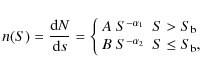 |
(5) |
where
 is the normalization,
 is the bright end slope,
 the faint end slope,
  the break flux, and S the flux in units of 10-14 erg cm-2 s-1. Notice that, using the maximum likelihood method, the fit is not dependent on the data binning and therefore we are using the whole dataset. Moreover, the normalization A is not a parameter of the fit, but is obtained by imposing the condition that the number of expected
sources from the best fit model is equal to the total observed number.
the break flux, and S the flux in units of 10-14 erg cm-2 s-1. Notice that, using the maximum likelihood method, the fit is not dependent on the data binning and therefore we are using the whole dataset. Moreover, the normalization A is not a parameter of the fit, but is obtained by imposing the condition that the number of expected
sources from the best fit model is equal to the total observed number.
In the 0.5-2 keV energy band the best fit parameters are
 ,
,
 ,
,
 erg cm-2 s-1 and A=141.
These values are consistent with those measured in Paper II while the normalization is lower than the value (A=198) derived in Paper II
erg cm-2 s-1 and A=141.
These values are consistent with those measured in Paper II while the normalization is lower than the value (A=198) derived in Paper II![]() . However, with this fitting method
the normalization is not a fit parameter and it is strongly dependent on the best fit values of the bright end slope and on the cut-off flux. One can indeed notice that the best fit values of the
and
parameters are somewhat changed with respect to Paper II.
The bright end slope varied from 2.6 in Paper II to 2.4 in the present
work and the cut-off flux varied from
. However, with this fitting method
the normalization is not a fit parameter and it is strongly dependent on the best fit values of the bright end slope and on the cut-off flux. One can indeed notice that the best fit values of the
and
parameters are somewhat changed with respect to Paper II.
The bright end slope varied from 2.6 in Paper II to 2.4 in the present
work and the cut-off flux varied from
 erg cm-2 s-1 to
 erg cm-2 s-1. However, a comparison of the amplitude of the source surface density measured in Paper II with that measured here can be performed if we measure the model predicted source counts at
fluxes fainter than the knee. If we take
erg cm-2 s-1. However, a comparison of the amplitude of the source surface density measured in Paper II with that measured here can be performed if we measure the model predicted source counts at
fluxes fainter than the knee. If we take
 erg cm-2 s-1 as a reference flux,
in Paper II we had a source surface density of 478 deg-2 while here we
measure 479 deg-2. We can therefore conclude that the 0.5-2 keV
obtained in Paper II and in this work are in good agreement.
erg cm-2 s-1 as a reference flux,
in Paper II we had a source surface density of 478 deg-2 while here we
measure 479 deg-2. We can therefore conclude that the 0.5-2 keV
obtained in Paper II and in this work are in good agreement.
In the 2-10 keV band the best fit parameters are
 ,
,
 ,
,
 10-14erg cm-2 s-1 and A=413.
Since the best fit parameters are similar to those of Paper II, we can directly
compare the normalizations of the
.
The normalization derived in this work
is 10% higher than that measured in Paper II. This effect is partly due to
the sources missing in the 2-4.5 keV band and detected in the 2-8 keV
which were not considered in the analysis of Paper II. Moreover, extrapolation of
the 2-4.5 keV count-rate into the broader 2-10 keV band
is more affected by uncertainties on the true source spectral slope and provides wrong
count-rate estimates especially for the most absorbed sources.
10-14erg cm-2 s-1 and A=413.
Since the best fit parameters are similar to those of Paper II, we can directly
compare the normalizations of the
.
The normalization derived in this work
is 10% higher than that measured in Paper II. This effect is partly due to
the sources missing in the 2-4.5 keV band and detected in the 2-8 keV
which were not considered in the analysis of Paper II. Moreover, extrapolation of
the 2-4.5 keV count-rate into the broader 2-10 keV band
is more affected by uncertainties on the true source spectral slope and provides wrong
count-rate estimates especially for the most absorbed sources.
![\begin{figure}
\par\includegraphics[width=8cm,clip]{0794fig8.ps}
\end{figure}](/articles/aa/full_html/2009/14/aa10794-08/img392.png) |
Figure 7:
The 2-10 keV
|
| Open with DEXTER | |
Table 4: Source number counts.
![\begin{figure}
\par\includegraphics[width=8cm,clip]{0794fig9.ps}
\end{figure}](/articles/aa/full_html/2009/14/aa10794-08/img450.png) |
Figure 8:
The 5-10 keV
|
| Open with DEXTER | |
In the 5-10 keV energy band we did not find any significant break in the slope. We therefore
fitted the data using a single power-law in the form of
 and
obtained
and
obtained
 and A=130.
In the 5-10 keV both the normalization and the slope are consistent within 1
with the values obtained in Paper II.
4.1 Comparison with previous surveys
In Figs. 6-8 we compare our
with the results of previous surveys. A visual inspection of the data shows that the XMM-COSMOS source counts are in general agreement, within 1,
with all the previous measurements.
In the 0.5-2 keV band source counts of all the surveys agree with our measurements,
with the only exception of the bright end of the Lockman Hole
.
The reason for such a discrepancy is that the location of the Lockman Hole survey was
chosen on purpose near a concentration of bright sources to improve
the accuracy of the ROSAT star tracker in order to achieve a
better astrometry (Hasinger, private communication).
This had the result of artificially increasing the source counts at the bright end of the relation. The comparison with other surveys is consistent with the error bars
and with the counts in cell fluctuations predicted in Paper II. We also compared our results with the recent work of Mateos et al. (2008) who performed a detailed analysis of the
of X-ray sources detected in 1129 XMM-Newton archival observations. By comparing the data of Table 4 with those shown in Table 3 of Mateos et al. (2008) we found 1
agreement in almost all the data bins.
In Paper II we showed that the fluctuations of the source counts
are proportional to the actual number of sources in the field and to the amplitude of the
angular auto-correlation function of the X-ray sources. Therefore, assuming a universal
shape of the autocorrelation function,
we expect that the surveys showing the largest deviations from the mean value
of the source density are the pencil beam surveys (i.e. area <0.2 deg2) at their bright end.
Moreover, with XMM-COSMOS , fluctuations introduced in previous shallow surveys by low counting statistics and
by random sampling of a few large structures in pencil beam surveys are largely suppressed.
With the same formulas used in Paper II,
we estimate the effect of the cosmic variance to be <5% on the normalization
of the XMM-COSMOS
and that the new data do not change the results shown in Paper II.
Also in the 2-10 keV energy bands we do not note any significant deviation from previous works with the exception only of the Lockman Hole and the two faintest bins of the AXIS counts. Also in this band our data are in good agreement with the results of Mateos et al. (2008).
Figure 8 suggests that the fluctuations of the source counts in the 5-10 keV band are much larger than in the other bands. This is due to the fact that as discussed above and in Paper II, when we deal with low source surface density, the impact of the sample variance becomes significantly high. However in this band our data are statistically consistent with most of the data from other surveys. Also in this energy band, the deviation of the COSMOS data from those of the Lockman Hole is due the higher number of bright sources in that particular field. Our source counts are 10-15% higher than those of the ELAIS-S1 survey (Puccetti et al. 2006). As an example, using Eq. (10) of Paper II, we determine that at the faint end of the 5-10 keV band, fluctuations due to the cosmic variance are of the order of the 20-40 percent, depending on the survey size. At the bright end large deviations of more than a factor of two are still allowed by the sample variance. This is also visible in Fig. 8 where at the bright end the Beppo-SAX counts exceed the XMM-COSMOS counts by about a factor of two though remaining statistically consistent with each other.
Kim et al. (2007) reported the results of a broken power law fit to the
from different surveys available in the literature. They also reported measurements of the CHAMP survey which is a compilation of Chandra archival data for a total sky coverage of 9.6 deg2,
with a depth about one order of magnitude fainter than XMM-COSMOS.
On average the bright end slopes are consistent with a Euclidean rise in all the surveys.
The faint end slopes are of the order of
 -1.6 in the 0.5-2 keV band and
span from
-1.6 in the 0.5-2 keV band and
span from
 to
to
 with a mean of
 -1.7.
A larger spread is reported for the cut off fluxes. Although the spread in this parameter is quite large, our data are consistent with the average values reported in the literature for this parameter.
-1.7.
A larger spread is reported for the cut off fluxes. Although the spread in this parameter is quite large, our data are consistent with the average values reported in the literature for this parameter.
4.2 Extragalactic X-ray source number counts and comparison with models
![\begin{figure}
\par\includegraphics[width=8cm,clip]{0794fig10.ps}
\end{figure}](/articles/aa/full_html/2009/14/aa10794-08/img457.png) |
Figure 9: The 0.5-2 keV flux distribution of sources classified as AGN or extragalactic (black) and stars (red). |
| Open with DEXTER | |
![\begin{figure}
\par\includegraphics[width=7.5cm]{0794fig11a.ps}\par\includegraphics[width=7.5cm]{0794fig11b.ps}
\end{figure}](/articles/aa/full_html/2009/14/aa10794-08/img458.png) |
Figure 10:
Upper panel: the ratio between the Gilli et al. (2007) model
|
| Open with DEXTER | |
We used our
relations to test the most recent extragalactic XRB synthesis models.
In order to compare our data with the XRB model, we estimate the fraction of sources classified as stars by Brusa et al. (2009). In the 0.5-2 keV band we identified 74/1621 (i.e. 4.5%) sources classified as stars, while these are 17/1111 (i.e. 1.5%) and 3/251 (i.e. 1.1%)
in the 2-10 keV and 5-10 keV bands, respectively.
In Fig. 9 we plot the normalized distributions of the fluxes of stars and extragalactic sources in the 0.5-2 keV band. Since the two distributions are similar we can conclude that stars in the XMM-COSMOS flux range affect the 0.5-2 keV
only by
increasing the extragalactic source counts by 5%. Mateos et al. (2008) measured a flux dependent fraction of stars, with higher fractions than ours at bright fluxes where XMM-COSMOS is undersampled.
By excluding the source classified as stars, we derived the
relations for extragalactic sources only.
In the upper panel of Fig. 10 we plot the ratio of the XMM-COSMOS
relations to the predictions of the XRB population synthesis model of Gilli et al. (2007,
hereafter model I), while in the bottom panel we plot for comparison the ratio of the data to
the model of Treister & Urry (2006) (hereafter model II).
In both models the XRB spectrum is dominated by obscured AGN
which outnumber unobscured ones by a factor 3-4 at low X-ray luminosities
(
 ). The cosmological evolution is similar and parametrized using
the most recent determinations of the AGN luminosity function
(Ueda et al. 2003; La Franca et al. 2005; Hasinger et al. 2005).
In both models the obscured fraction decreases towards high luminosity.
The luminosity dependence is stronger in Treister et al. (2006)
who also allow the obscured fraction to increase at high redshifts.
The absorption distribution is peaked around
). The cosmological evolution is similar and parametrized using
the most recent determinations of the AGN luminosity function
(Ueda et al. 2003; La Franca et al. 2005; Hasinger et al. 2005).
In both models the obscured fraction decreases towards high luminosity.
The luminosity dependence is stronger in Treister et al. (2006)
who also allow the obscured fraction to increase at high redshifts.
The absorption distribution is peaked around
 in Gilli
et al. (2007), while it remains rather flat above
in Gilli
et al. (2007), while it remains rather flat above
 in Treister
et al. (2006). They also differ in the adopted XRB intensity around the 30 keV peak.
The Gilli et al. (2007) model is tuned to fit the HEAO-1 level, consistent,
within 10%, with recent BeppoSAX (Frontera et al. 2007) and Swift BAT
(Ajello et al. 2008) measurements, while Treister et al. renormalize
the HEAO-1 intensity upward by a factor 1.4 to better match the extrapolation
of lower energy (<10 keV) data (i.e. De Luca & Molendi 2004).
Moreover, for this paper we adopt a modified version of the Gilli et al. (2007) model
in Treister
et al. (2006). They also differ in the adopted XRB intensity around the 30 keV peak.
The Gilli et al. (2007) model is tuned to fit the HEAO-1 level, consistent,
within 10%, with recent BeppoSAX (Frontera et al. 2007) and Swift BAT
(Ajello et al. 2008) measurements, while Treister et al. renormalize
the HEAO-1 intensity upward by a factor 1.4 to better match the extrapolation
of lower energy (<10 keV) data (i.e. De Luca & Molendi 2004).
Moreover, for this paper we adopt a modified version of the Gilli et al. (2007) model![]() which takes into account the decline of the space density of AGN at z > 3 discussed by Brusa et al. (2008). In order to test the models over a wider range of fluxes we also plotted the data of the CDFN (Bauer et al. 2004) and CDFS (Luo et al. 2008) surveys. By restricting our analysis to fluxes larger than 10-16 erg cm-2 s-1, the contribution of normal galaxy counts is negligible (Ranalli et al. 2003). The results of this comparison can be summarized as follows:
which takes into account the decline of the space density of AGN at z > 3 discussed by Brusa et al. (2008). In order to test the models over a wider range of fluxes we also plotted the data of the CDFN (Bauer et al. 2004) and CDFS (Luo et al. 2008) surveys. By restricting our analysis to fluxes larger than 10-16 erg cm-2 s-1, the contribution of normal galaxy counts is negligible (Ranalli et al. 2003). The results of this comparison can be summarized as follows:
- in the 5-10 keV energy band, both models reproduce well the XMM-COSMOS
,
while the CDFS counts show a systematically different slope from that of the predicted relation. However, because of the small effective area of Chandra above 5 keV (i.e. 200 cm2 at 6.4 keV), the 5-10 keV CDFS
may suffer from significant systematic uncertainties.
- in the 2-10 keV energy band, the models reproduce quite accurately the
XMM-COSMOS data, although model II slightly (i.e. 10%) overpredicts the XMM-COSMOS counts. The CDFN counts show a systematically higher normalization than those of the models (up to 40% at faint fluxes) and of the COSMOS and CDFS data.
- in the 0.5-2 keV band both models show significant deviations from both data sets.
Source counts estimated from model I show a systematically steeper slope than the data. On average, model I deviates from the observations by about 10-15% in the flux range 10-16 erg cm-2 s-1-10-13 erg cm-2 s-1. Model II, on the other hand, systematically
underestimates the source counts while a visual inspection shows a good
agreement with the observed slopes. In this case deviations
between the data and the model are of the order of 20% at the XMM-COSMOS fluxes, while at fainter fluxes the deviations are larger and of the order of 30%-40%. Both models underestimate the observed counts by 30% at fluxes greater than 10-14 erg cm-2 s-1
10%. In the soft band the agreement between the predicted and the
observed relations is not as good as in the harder energy bands20%) and such that it can be easily accommodated by slight variations of the XRB model parameters. This band is in fact more sensitive to the effect of absorption and therefore a fine
tuning of absorption in AGN is required in the models. Moreover, this band contains a larger fraction of high-z objects (Brusa et al. 2009). Therefore, the fact that the two models assume a somewhat different absorption evolution and XRB spectrum can, in the first instance,
explain the different source count predictions. We can conclude that at the flux limits of the XMM-COSMOS survey, XRB synthesis models can reproduce the observations with a precision of 10%-20%.
5 X-ray colours of the X-ray sources
The X-ray colours or hardness ratios are defined as
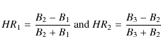 |
(6) |
where B1, B2, and B3 refer to the vignetting-corrected count rates in the 0.5-2 keV, 2-10 keV and 5-10 keV bands, respectively. By construction, both HR1 and HR2 can assume values between -1 and 1.
Figure 11 displays the HR1-HR2 plot of 212 sources for which the 1
error on both HR1 and HR2 is <0.25 and for which a high quality optical spectrum is available.
The plot also contains a grid of the expected values of HR1 and HR2 for different spectral models.
In particular we considered a simple power law model with a spectral index in the interval
 and with a column density (
 cm-2.
cm-2.
![\begin{figure}
\par\includegraphics[width=8cm,clip]{0794fig12.ps}
\end{figure}](/articles/aa/full_html/2009/14/aa10794-08/img468.png) |
Figure 11:
X-ray colour-colour diagram in the XMM-COSMOS survey. Colours are defined in the text. XID #2608 has been plotted with its error which also represents the typical amplitude of the uncertainties in the plot. The grid represents the places in the HR1-HR2 plane of sources with single power-law spectra with
|
| Open with DEXTER | |
 3 with absorption with a column density
 cm-2. The green line marks the region occupied by candidate Compton thick-AGN [i.e.
  ]
and the marks on top of it represent 1%, 3% 10% and 30% level of leaking flux, from top to bottom. We represent type I AGN, type II AGN, emission line and absorption line galaxies as
blue filled circles,
red empty triangles,
cyan empty exagons,
green filled squares,respectively.
]
and the marks on top of it represent 1%, 3% 10% and 30% level of leaking flux, from top to bottom. We represent type I AGN, type II AGN, emission line and absorption line galaxies as
blue filled circles,
red empty triangles,
cyan empty exagons,
green filled squares,respectively.
![\begin{figure}
\par\includegraphics[width=8cm,clip]{0794fig13.ps}
\end{figure}](/articles/aa/full_html/2009/14/aa10794-08/img469.png) |
Figure 12: The 2-10 keV X-ray luminosity vs. HR1 for the sources fullfilling the HR error selection. We represent type I AGN, type II AGN, emission line and absorption line galaxies as blue filled circles, red empty triangles, cyan empty exagons, green filled squares,respectively. |
| Open with DEXTER | |
In Brusa et al. (2009), and Trump et al. (2008), extragalactic sources are classified into 4 main categories:
- type I AGN, if the optical spectrum shows evidence of broad (FWHM>2000 km s-1) emission lines;
- type II AGN, if the optical spectrum shows evidence of narrow, high-ionization emission lines and/or AGN diagnostic diagrams;
- emission line galaxy, if the optical spectrum is dominated by a galaxy continuum plus emission lines but without secure AGN indicators;
- absorption line galaxy if the optical spectrum is dominated by a galaxy continuum plus absorption lines.
(
 erg/s, with most of them having
 erg/s (see Fig. 12). The adopted cuts on the errors on the HR preferentially select unabsorbed to moderate absorbed AGN, biasing the sample against normal galaxies, starforming galaxies and the most obscured AGN.
type I AGN (
blue filled circles) cluster in a region around
 and
and
 with a relatively small dispersion, corresponding to a typical X-ray spectrum dominated by a power-law continuum with very low absorption. Only a few type I sources have X-ray colours typical of type II sources (i.e.
 which corresponds to
NH>1022 cm-2). This fraction (2%) is consistent with the results from X-ray spectral analysis on a subsample of XMM-COSMOS sources (Mainieri et al. 2007) but at variance with previous works on the fraction of X-ray absorbed type I AGN at comparable X-ray luminosity (see e.g. Brusa et al. 2003; Perola et al. 2004; Page et al. 2004) which reported values as large as 10%. However such a low fraction may be a consequence of the selection effect mentioned above.
which corresponds to
NH>1022 cm-2). This fraction (2%) is consistent with the results from X-ray spectral analysis on a subsample of XMM-COSMOS sources (Mainieri et al. 2007) but at variance with previous works on the fraction of X-ray absorbed type I AGN at comparable X-ray luminosity (see e.g. Brusa et al. 2003; Perola et al. 2004; Page et al. 2004) which reported values as large as 10%. However such a low fraction may be a consequence of the selection effect mentioned above.
On the other hand, type II AGN (
red empty triangles) fill most of the HR1-range, corresponding
to observed frame absorption up to 1023 cm2. The fraction of type II AGN with X-ray colours typical of type I AGN (
 )
is 30%. This is consistent with the fraction of X-ray unobscured type II AGN reported in Mainieri et al. (2007).
)
is 30%. This is consistent with the fraction of X-ray unobscured type II AGN reported in Mainieri et al. (2007).
An interesting source is XID = #2608 which has been classified as a
Compton-Thick AGN by Mainieri et al. (2007) and Hasinger et al. (2007) but its optical spectrum is that of an emission line galaxy. In Hasinger et al. (2007) a small number of sources (including XID = #2608)
was found to have hardness ratios that could be interpreted as being due to heavily absorbed (possibly Compton thick) high energy spectra with some fraction of leaking
unabsorbed soft flux. The solid green line
in Fig. 11 represents the expected
tracks occupied by leaking Compton thick sources
in the HR1-HR2 plane![]() at z=0. The line has been computed with a pure reflection model with a fraction
of 1%, 3%, 10% and 30% (from top to bottom) of the flux from the central source leaking out.
at z=0. The line has been computed with a pure reflection model with a fraction
of 1%, 3%, 10% and 30% (from top to bottom) of the flux from the central source leaking out.
In particular the source ID = #2608 shows
X-ray colours typical of a spectrum dominated by
a pure reflection component with 3% of the original flux leaking out.
Another source, XID = #131, shows X-ray colours consistent with Compton-thick AGN with a
small fraction of leaking flux. We note that a 1% fraction of Compton-thick AGN is
consistent with the predictions of XRB models at the flux limit of this subsample (i.e. 2-10 keV flux >10-14 erg cm-2 s-1) and with the source counts of Compton-thick objects measured in a collection of surveys by Brunner et al. (2008).
The objects classified as emission and absorption line galaxies are spread over the entire luminosity-hardness ratio plane (see Fig. 12) and their nature can be explained as a mixture of star forming galaxies, type II AGN and XBONGs (see e.g. Comastri et al. 2002; Cocchia et al. 2007; Civano et al. 2007; Caccianiga et al. 2007). A more detailed analysis of their multiwavelength properties will be the subject of a forthcoming publication.
6 Summary
In this paper we presented a pointlike source catalogue in the XMM-COSMOS survey. The survey
covers an area of 2.13 deg2 in the equatorial sky. The field has been observed with 55 XMM-Newton pointings for a total exposure time of 1.5 Ms. We achieved an almost uniform exposure of 40 ks on the field.
We detected a total number of 1621, 1111 and 251 sources in the 0.5-2 keV,
2-10 keV and 5-10 keV energy band, respectively, for a total of 1887 independent sources detected with det_ml > 10 in at least one band. The survey has a limiting flux of
erg cm-2 s-1,
erg cm-2 s-1 and
erg cm-2 s-1 in the 0.5-2 keV, 2-10 keV and 5-10 keV energy band, over 90% of the area.
Together with the source catalogue we derived
relations with high statistics
in the flux interval sampled by the survey. The
relations
are in good agreement with most of the X-ray surveys published in the
literature. We compared our source counts with the most recent XRB population synthesis
models (Gilli et al. 2007; Treister & Urry 2006) and found that they agree within 10% with our data
in the 5-10 keV and 2-10 keV energy bands. In the 0.5-2 keV band
both models deviate from the XMM-COSMOS data by about 10%-30% suggesting, that further
improvements in the modeling are required. We isolated a subsample of X-ray bright sources for which optical spectroscopy is available. About 65% of them have optical and X-ray properties typical of type I AGN and 15% of type II AGN. In the subsample of sources with a good optical spectrum and good counting statistics, the number of candidate Compton thick (1-2) AGN is fully consistent with the expectations of XRB population synthesis models. By combining X-ray colours and optical spectroscopy we found that 20% of the sources do not show, in the optical band, evident signatures of AGN activity although their X-ray luminosities are typical of AGN. Additonally, we consider XMM-COSMOS as a pathfinder for the eROSITA (Predehl et al. 2006) X-ray telescope which will be launched in 2012 and that will perform an all sky survey with sensitivities comparable to those presented here.
Acknowledgements
Part of this work was supported by the German Deutsche Forschungsgemeinschaft, DFG project number Ts 17/2-1.In Germany the XMM-Newton project is supported by the Bundesministerium für Wirtshaft und Techologie/Deutsches Zentrum für Luft und Raumfahrt and the Max-Planck society. N.C. and A.F. were partially supported from a NASA grant NNX07AV03G to UMBC. In Italy, the XMM-COSMOS project is supported by PRIN/MIUR under grant 2006-02-5203 and ASI-INAF grants I/023/05/00, I/088/06. Part of this work was supported by the German Deutsche Forschungsgemeinschaft,DFG Leibniz Prize (FKZ HA 1850/28-1). N.C. gratefully acknowledges Ezequiel Treister for providing his prediction of the XRB
References
- Ajello, M., et al. 2008, [arXiv:0808.3377]
- Baldi, A., Molendi, S., Comastri, A., et al. 2002, ApJ, 564, 190 In the text
- Bauer, F. E., Alexander, D. M., Brandt, W. N., et al. 2004, AJ, 128, 2048 In the text
- Branchesi, M., Gioia, I. M., Fanti, C., Fanti, R., & Cappelluti, N. 2007, A&A, 462, 449 In the text
- Brunner, H., Cappelluti, N., Hasinger, G., et al. 2008, A&A, 479, 283 In the text
- Brandt, W. N., & Hasinger, G. 2005, ARA&A, 43, 827 In the text
- Brusa, M., Comastri, A., Gilli, R., et al. 2008, [arXiv:0809.2513] In the text
- Brusa, M., et al. 2009, A&A, in preparation In the text
- Caccianiga, A., Severgnini, P., Della Ceca, R., et al. 2007, A&A, 470, 557 In the text
- Cagnoni, I., della Ceca, R., & Maccacaro, T. 1998, ApJ, 493, 54 In the text
- Cappelluti, N., Cappi, M., Dadina, M., et al. 2005, A&A, 430, 39 In the text
- Cappelluti, N., Hasinger, G., Brusa, M., et al. 2007a, ApJS, 172, 341
- Cappelluti, N., Böhringer, H., Schuecker, P., et al. 2007b, A&A, 465, 35 In the text
- Cappi, M., Mazzotta, P., Elvis, M., et al. 2001, ApJ, 548, 624 In the text
- Carrera, F. J., Ebrero, J., Mateos, S., et al. 2007, A&A, 469, 27 In the text
- Cavaliere, A., & Fusco-Femiano, R. 1976, A&A, 49, 137 In the text
- Civano, F., Mignoli, M., Comastri, A., et al. 2007, A&A, 476, 1223 In the text
- Cocchia, F., Fiore, F., Vignali, C., et al. 2007, A&A, 466, 31 In the text
- Comastri, A., Mignoli, M., Ciliegi, P., et al. 2002, ApJ, 571, 771 In the text
- Della Ceca, R., Maccacaro, T., Caccianiga, A., et al. 2004, A&A, 428, 383 In the text
- De Luca, A., & Molendi, S. 2004, A&A, 419, 837
- Elvis, M., et al. 2009, [arXiv:0903.2062] In the text
- Finoguenov, A., Guzzo, L., Hasinger, G., et al. 2007, ApJS, 172, 182
- Finoguenov, A., et al. 2008, ApJ, in preparation In the text
- Fiore, F., Giommi, P., Vignali, C., et al. 2001, MNRAS, 327, 771 In the text
- Fiore, F., Brusa, M., Cocchia, F., et al. 2003, A&A, 409, 79
- Frontera, F., Orlandini, M., Landi, R. et al. 2007, ApJ, 666, 86
- Gilli, R., Comastri, A., & Hasinger, G. 2007, A&A, 463, 79 In the text
- Giommi, P., Perri, M., & Fiore, F. 2000, A&A, 362, 799 In the text
- Hasinger, G., Burg, R., Giacconi, R., et al. 1993, A&A, 275, 1 In the text
- Hasinger, G., Miyaji, T., & Schmidt, M. 2005, A&A, 441, 417 In the text
- Hasinger, G., Cappelluti, N., Brunner, H., et al. 2007, ApJS, 172, 29 In the text
- Hathaway, D. H., Wilson, R. M., & Reichmann, E. J. 1999, J. Geophys. Res., 104, 22375 In the text
- Kenter, A., Murray, S. S., Forman, W. R., et al. 2005, ApJS, 161, 9
- Kim, M., Kim, Dong-Woo, Wilkes, B. J., et al. 2007, ApJS, 169, 401 In the text
- Kocevski, D. D., Lubin, L. M., Gal, R., et al. 2008, [arXiv:0804.1955] In the text
- La Franca, F., Fiore, F., Comastri, A., et al. 2005, ApJ, 635, 864
- Lehmer, B. D., Brandt, W. N., Alexander, D. M., et al. 2005, ApJS, 161, 21 In the text
- Luo, B., et al. 2008, [arXiv:0806.3968] In the text
- Mainieri, V., Hasinger, G., Cappelluti, N., et al. 2007, ApJS, 172, 368 In the text
- Mainieri, V., et al. 2009, A&A, in preparation In the text
- Mateos, S., et al. 2008, [arXiv:0809.1939] In the text
- McCracken, H. J., Peacock, J. A., Guzzo, L., et al. 2007, ApJS, 172, 314 In the text
- Moretti, A., Campana, S., Lazzati, D., & Tagliaferri, G. 2003, ApJ, 588, 696 In the text
- Narsky, I. 2000, Nucl. Instr. Meth. Phys. Res. A, 450, 444 In the text
- Page, M. J., Stevens, J. A., Ivison, R. J., & Carrera, F. J. 2004, ApJ, 611, L85
- Panessa, F., & Bassani, L. 2002, A&A, 394, 435
- Perola, G. C., Puccetti, S., Fiore, F., et al. 2004, A&A, 421, 491
- Predehl, P., Hasinger, G., Böhringer, H., et al. 2006, Proc. SPIE, 6266 In the text
- Puccetti, S., Fiore, F., D'Elia, V., et al. 2006, A&A, 457, 501 In the text
- Ranalli, P., Comastri, A., & Setti, G. 2003, A&A, 399, 39 In the text
- Rosati, P., Giacconi, R., Gilli, R., et al. 2002, ApJ, 566, 667 In the text
- Salvato, M., et al. 2008, [arXiv:0809.2098]
- Scoville, N., Aussel, H., Brusa, M., et al. 2007, ApJS, 172, 1 In the text
- Schmitt, J. H. M. M., & Maccacaro, T. 1986, ApJ, 310, 334 In the text
- Szokoly, G. P., Bergeron, J., Hasinger, G., et al. 2004, ApJS, 155, 271
- Treister, E., & Urry, C. M. 2006, ApJ, 652, L79 In the text
- Trump, J. R., et al. 2008, [arXiv:0811.3977] In the text
- Ueda, Y., Akiyama, M., Ohta, K., & Miyaji, T. 2003, ApJ, 598, 886
Footnotes
- ... catalogue
- Based on observations obtained with XMM-Newton, an ESA science mission with instruments and contributions directly funded by ESA Member States and NASA. Based on observations obtained with MegaPrime/MegaCam, a joint project of CFHT and CEA/DAPNIA, at the Canada-France-Hawaii Telescope (CFHT) which is operated by the National Research Council (NRC) of Canada, the Institut National des Sciences de l'Univers of the Centre National de la Recherche Scientifique (CNRS) of France, and the University of Hawaii. This work is based in part on data products produced at TERAPIX.
- ...
- Full Table 3 is only available in electronic form at the CDS via anonymous ftp to cdsarc.u-strasbg.fr (130.79.128.5) or via http://cdsweb.u-strasbg.fr/cgi-bin/qcat?J/A+A/497/635
- ...
- Similar results also have been obtainedvia Monte Carlo simulations.
- ... ECFs
- The ECF values also take into account the energy channels discarded to decrease the background.
- ...
- We checked that a 30
aperture gives the best agreement between aperture photometry and the maximum likelihood PSF fitting technique.
- ... (cts/pix)
- The pixel scale is 4''/pix.
- ... catalogue
- We kept these sources as single entries in the catalog for self consistency with our statistical analysis.
- ... Paper II
- Note that in Paper II we gave the normalization of the cumulative distributions.
- ... model
- The predictions of the model can be retrieved on line at http://www.oabo.inaf.it/~gilli/counts.html using the POMPA COUNTS software (POrtable Multi Purpose Application for the AGN COUNTS).
- ... bands
- Note that the inclusion of a decline in the space density of AGN at high-z in model I affects mostly the 0.5-2 keV energy bands. In the harder bands the predicted number counts are comparable with or without a high-z space density decline.
- ... plane
- The position in this HR1-HR2 plane of the track of leaking Compton thick objects is different from that shown in Hasinger et al. (2007) because of the difference in the energy range of the hard band (i.e. 2-8 keV here, 2-4.5 keV in Hasinger et al. 2007).
All Tables
Table 1: The XMM- Newton observation log of the XMM-COSMOS survey.
Table 2: Summary of the total detections, single band detections, faintest flux limits, flux limits at 50%, 90% of the total area and flux limits observable on the full area in the 0.5-2 keV, 2-10 keV and 5-10 keV energy bands, respectively.
Table 3: Extract of the source catalogue.
Table 4: Source number counts.
All Figures
| |
Figure 1:
Colour coded vignetting corrected 0.5-2 keV exposure map of the XMM-COSMOS survey. The maximum effective depth achieved on the field is |
| Open with DEXTER | |
| In the text | |
| |
Figure 2: False colour X-ray image of the COSMOS field: red, green and blue colours represent the 0.5-2 keV, 2-4.5 keV and 4.5-10 keV energy bands, respectively. |
| Open with DEXTER | |
| In the text | |
| |
Figure 3: The distribution of the positional uncertainties of the XMM-COSMOS detections. |
| Open with DEXTER | |
| In the text | |
| |
Figure 4:
The region (
|
| Open with DEXTER | |
| In the text | |
| |
Figure 5:
Left panel: the sky coverage versus flux for the 0.5-2 keV, 2-10 keV and 5-10 keV bands, represented by red, green and blue solid lines. The horizontal solid and dashed lines show the 90% and 50% completeness levels. Right panel: the 0.5-2 keV sensitivity map of XMM-COSMOS in erg cm-2 s-1. The map is plotted in colour coded scale from
|
| Open with DEXTER | |
| In the text | |
| |
Figure 6:
The 0.5-2 keV
|
| Open with DEXTER | |
| In the text | |
| |
Figure 7:
The 2-10 keV
|
| Open with DEXTER | |
| In the text | |
| |
Figure 8:
The 5-10 keV
|
| Open with DEXTER | |
| In the text | |
| |
Figure 9: The 0.5-2 keV flux distribution of sources classified as AGN or extragalactic (black) and stars (red). |
| Open with DEXTER | |
| In the text | |
| |
Figure 10:
Upper panel: the ratio between the Gilli et al. (2007) model
|
| Open with DEXTER | |
| In the text | |
| |
Figure 11:
X-ray colour-colour diagram in the XMM-COSMOS survey. Colours are defined in the text. XID #2608 has been plotted with its error which also represents the typical amplitude of the uncertainties in the plot. The grid represents the places in the HR1-HR2 plane of sources with single power-law spectra with
|
| Open with DEXTER | |
| In the text | |
| |
Figure 12: The 2-10 keV X-ray luminosity vs. HR1 for the sources fullfilling the HR error selection. We represent type I AGN, type II AGN, emission line and absorption line galaxies as blue filled circles, red empty triangles, cyan empty exagons, green filled squares,respectively. |
| Open with DEXTER | |
| In the text | |
Copyright ESO 2009
Current usage metrics show cumulative count of Article Views (full-text article views including HTML views, PDF and ePub downloads, according to the available data) and Abstracts Views on Vision4Press platform.
Data correspond to usage on the plateform after 2015. The current usage metrics is available 48-96 hours after online publication and is updated daily on week days.
Initial download of the metrics may take a while.