| Issue |
A&A
Volume 495, Number 2, February IV 2009
|
|
|---|---|---|
| Page(s) | 587 - 606 | |
| Section | The Sun | |
| DOI | https://doi.org/10.1051/0004-6361:200810143 | |
| Published online | 04 December 2008 | |
High-precision density measurements in the solar corona
I. Analysis methods and results for Fe XII and Fe XIII
P. R. Young1,2,3,![]() -
T. Watanabe4 -
H. Hara4 -
J. T. Mariska3
-
T. Watanabe4 -
H. Hara4 -
J. T. Mariska3
1 - Rutherford Appleton Laboratory, Chilton, Didcot,
Oxfordshire OX11 0QX, UK
2 -
George Mason University, 4400 University Drive, Fairfax, VA 22030, USA
3 -
Space Science Division, Naval Research Laboratory,
Washington, DC 20375, USA
4 -
National Astronomical Observatory of Japan, National
Institutes of Natural Sciences, Mitaka, Tokyo 181-8588, Japan
Received 6 May 2008 / Accepted 26 September 2008
Abstract
Aims. The EUV Imaging Spectrometer (EIS) instrument on board the Hinode satellite has access to some of the best coronal density diagnostics, and the high sensitivity of the instrument now allows electron number density, ![]() ,
measurements to an unprecedented precision of up to
,
measurements to an unprecedented precision of up to ![]() % in active regions. This paper gives a thorough overview of data analysis issues for the best diagnostics of Fe XII and Fe XIII and assesses the accuracy of the measurements.
% in active regions. This paper gives a thorough overview of data analysis issues for the best diagnostics of Fe XII and Fe XIII and assesses the accuracy of the measurements.
Methods. Two density diagnostics each from Fe XII (![]() 186.88/
186.88/![]() 195.12 and
195.12 and ![]() 196.64/
196.64/![]() 195.12) and Fe XIII (
195.12) and Fe XIII (![]() 196.54/
196.54/![]() 202.04 and
202.04 and ![]() 203.82/
203.82/![]() 202.04) are analysed in two active region datasets from 2007 May 3 and 6 that yield densities in the range
202.04) are analysed in two active region datasets from 2007 May 3 and 6 that yield densities in the range
![]() .
The densities are derived using v5.2 of the CHIANTI atomic database. Blending, line fitting, and instrumental issues are discussed, and line fit parameters presented.
.
The densities are derived using v5.2 of the CHIANTI atomic database. Blending, line fitting, and instrumental issues are discussed, and line fit parameters presented.
Results. The Fe XII and Fe XIII diagnostics show broadly the same trend in density across the active region, consistent with their similar temperatures of formation. However, the high precision of the EIS measurements demonstrates significant discrepancies of up to 0.5 dex in derived
![]() values, with Fe XII always giving higher densities than Fe XIII. The discrepancies may partly be due to real physical differences between the emitting regions of the two plasmas, but the dominant factor lies in the atomic models of the two ions. Two specific problems are identified for Fe XII
values, with Fe XII always giving higher densities than Fe XIII. The discrepancies may partly be due to real physical differences between the emitting regions of the two plasmas, but the dominant factor lies in the atomic models of the two ions. Two specific problems are identified for Fe XII ![]() 196.64 and Fe XIII
196.64 and Fe XIII ![]() 203.82: the former is found to be underestimated in strength by the CHIANTI atomic model, while the high-density limit of the
203.82: the former is found to be underestimated in strength by the CHIANTI atomic model, while the high-density limit of the ![]() 203.82/
203.82/![]() 202.04 ratio appears to be inaccurate in the CHIANTI atomic model. The small grating tilt of the EIS instrument is found to be very significant when deriving densities from emission lines separated by more than a few angstroms. Revised wavelengths of
202.04 ratio appears to be inaccurate in the CHIANTI atomic model. The small grating tilt of the EIS instrument is found to be very significant when deriving densities from emission lines separated by more than a few angstroms. Revised wavelengths of
![]() Å and
Å and
![]() Å are suggested for the Fe XIII
Å are suggested for the Fe XIII ![]() 196.54 and Fe XII
196.54 and Fe XII ![]() 196.64 lines, respectively.
196.64 lines, respectively.
Key words: Sun: corona - Sun: UV radiation
1 Introduction
Density is a fundamental plasma parameter that is accessible to astrophysical spectroscopists through the density diagnostic - a ratio of two emission lines that is sensitive to the electron density of the emitting plasma. High accuracy density measurements are of direct importance for constraining energy and pressure balance within coronal structures, and also of indirect importance to the measure of the `filling factor' of the plasma, i.e., the fraction (by volume) of the observed plasma structure that is actually emitting radiation. The latter is of significance when the spatial resolution of the telescope is not sufficient to resolve the physical structures of interest, as is often the case even for our nearest star. The power of emission line density diagnostics lies in the fact that, when the plasma is optically thin, the derived density depends purely on the atomic data for the emitting ion and is free of any physical assumptions about the volume, abundances or temperature structure within the plasma.
Density diagnostics for use in both analyses of stellar coronae and nebulae have been described and exploited for many years. For the solar corona, reviews of early work are provided by Dere & Mason (1981) and Mariska (1992). Steady improvements in the accuracy of atomic data calculations and access to high resolution, calibrated ultraviolet spectra from space-borne instruments have led to a number of detailed studies of density diagnostics from both individual ions and sequences of ions, e.g., Brickhouse et al. (1995), Laming et al. (1997) and Young et al. (1998).
A particular advance has been the routine access to most of the wavelength range 150-1600 Å by the CDS and SUMER instruments on board the SOHO spacecraft for over a 12 year period. A wide range of density diagnostics from many different ions has been exploited (e.g., Laming et al. 1997; Del Zanna & Mason 2003; Doschek et al. 1997; Young et al. 1999), however the density measurements from these two instruments are generally accurate only to the 30-40% level at best and often it is necessary to bin multiple spatial pixels or exposures to obtain a useful signal. This is because the most commonly-used diagnostics generally involve only weak-to-medium strength emission lines and/or the diagnostics themselves do not have high sensitivity to density.
The best density diagnostics at typical coronal temperatures (1-3 MK) belong to the set of iron ions Fe IX-XV. They arise because of the complex atomic structures of these ions which lead to a number of metastable levels that are the source of the density sensitivity of the emission line ratios (e.g., Sect. 6.3.1 of Dere & Mason 1981). The density diagnostics of these iron ions are mostly found below 300 Å, a wavelength region not well covered by the SOHO spectrometers.
The EUV Imaging Spectromer (EIS) on board the Hinode satellite - launched during 2006 September - observes two wavelength ranges below 300 Å and, for the first time, scientists have routine access to high spectral and spatial resolution data in this region. A key factor is the high sensitivity of the instrument which is enabled by a simple optical design that incorporates multilayer coatings (Culhane et al. 2007). The sensitivity is particularly high in the range 185-205 Å where are found excellent density diagnostics from Fe XII and Fe XIII. As demonstrated in the following sections, diagnostics from these ions yield density measurements with an unprecedented precision of up to 5% in individual spatial pixels at exposure times of 30 s or less - a vast improvement over earlier instruments.
The diagnostic potential of Fe XII and Fe XIII has been
recognised for many years. The first sophisticated atomic calculation
for Fe XII was performed by Flower (1977) and a number of UV
density diagnostics have been studied
(e.g., Feldman et al. 1983; Tayal et al. 1991), but for many years
there were large discrepancies between predictions from atomic data
models and measured
line intensities which were summarised in Binello et al. (2001). Finally
the large R-matrix calculation performed by Storey et al. (2005)
resolved many of the problems (Del Zanna & Mason 2005). The three emission
lines used in the present work (![]() 186.88,
186.88, ![]() 195.12 and
195.12 and ![]() 196.64)
were shown by Del Zanna & Mason (2005) to give good
agreement with other line
ratios from Fe XII, but each line is affected by line
blending. This will be discussed in detail during the course of the
present work.
196.64)
were shown by Del Zanna & Mason (2005) to give good
agreement with other line
ratios from Fe XII, but each line is affected by line
blending. This will be discussed in detail during the course of the
present work.
For Fe XIII, Flower & Nussbaumer (1974)
calculated atomic data and produced line ratio calculations that
yielded reasonably consistent density measurements from a quiet Sun
spectrum. Detailed comparisons of the more recent atomic data models of
Fe XIII in the CHIANTI atomic database (Dere et al. 1997) with
spectra from the SERTS rocket flight experiments (Neupert et al. 1992) have
been performed by Young et al. (1998) and Landi (2002). In particular,
the latter work found that the ![]() 196.54/
196.54/![]() 202.04 and
202.04 and
![]() 203.82/
203.82/![]() 202.04 ratios used in the present work give
density estimates in good agreement with each other and also with
other ions formed at similar tempera- tures.
202.04 ratios used in the present work give
density estimates in good agreement with each other and also with
other ions formed at similar tempera- tures.
Early density results from EIS obtained using the Fe XII and Fe XIII diagnostics have been presented in Brooks et al. (2007), Watanabe et al. (2007), Doschek et al. (2007a), Doschek et al. (2007b) and Dere et al. (2007). In particular we highlight the density maps shown in Doschek et al. (2007b) that demonstrate the high quality of the EIS density measurements, and the density comparisons shown in Watanabe et al. (2007) that show excellent agreement between four different iron ion density diagnostics.
In this paper density measurements from two diagnostics each of the Fe XII and Fe XIII ions are presented from two active region data sets. A careful discussion of line fitting and blending issues is given, and an estimate of the accuracy of the density measurements is made. A following paper will use the derived densities to estimate column depths and filling factors for the two ions.
Table 1: Transition information and CHIANTI wavelengths for the density diagnostics.
2 Instrument details
The EUV Imaging Spectrometer (EIS) on Hinode observes two
wavelength ranges: 170-212 Å and 246-292 Å. The instrument is
described in detail by Korendyke et al. (2006) and Culhane et al. (2007). The key
optical elements are: a parabolic primary mirror for focussing incoming
radiation; a uniform line-spaced grating for dispersing the radiation
and two back-thinned, EUV sensitive CCDs for detecting the
radiation. Two aluminium filters lie on the optical path for blocking
visible radiation, and a slit-slot assembly is situated between the
mirror and grating containing four different-sized slits for selecting
the spatial region to be sent to the spectromer. The optical surfaces
of both the mirror and grating are divided in two and coated with
multilayer coatings optimised for the two wavelength bands. Of the
four entrance slits, two are available for detailed
spectroscopy work with projected widths at the Sun of
1
![]() and 2
and 2
![]() .
Pixel sizes on the detector are 1
.
Pixel sizes on the detector are 1
![]() (spatial
dimension) and 0.0223 Å (spectral dimension). For single exposures
the maximum field-of-view in Solar-Y is 512
(spatial
dimension) and 0.0223 Å (spectral dimension). For single exposures
the maximum field-of-view in Solar-Y is 512
![]() .
.
For density measurements, the absolute radiometric calibration of the
EIS instrument is not important, only the relative calibration between
the wavelengths of the lines. The key uncertainty is whether the
relative reflectivities from the mirror and grating between two
wavelengths deviate from the values contained in the calibration
pipeline. There are two components: the uncertainty due to variations in
reflectivity across the optical surfaces; and a systematic error in
the reflectivity curves due to some change in the instrument between
the laboratory calibration measurements and launch.
For the former, measurements performed on flight-quality mirrors and gratings by
Seely et al. (2004) revealed that, when a beamline is scanned
across the optical surfaces, the reflectivity as a function of wavelength is
found to vary. Seely et al. (2004) averaged the resulting reflectivity
curves and the standard deviations of the data points for the
wavelengths considered here range from 3 to 8%. In orbit the optical
surfaces are fully illuminated which will serve to average out the
variations and so these standard deviation values will be over-estimates of
the actual uncertainty in the relative calibration. In addition, these
percentage errors are for the absolute reflectivity - the standard
deviation for the relative reflectivities between two lines close in
wavelength (e.g., the Fe XIII ![]() 202.04 and
202.04 and ![]() 203.82) will
likely be significantly less. For this reason we
do not include any estimate of the relative calibration uncertainty in
the error budget for derived densities. The error bars for
the density measurements presented here are thus underestimates,
but we believe the uncertainties in the relative calibration are
comparable to or smaller than these errors and would not significantly
impact the conclusions of this work. Of greater concern for the
present work is whether there is a systematic error in the shape of
the multilayer reflectivity curves used in the EIS calibration. This
can be investigated through the study of emission line ratios that are
insensitive to the plasma conditions - an example being the
Fe XII ratios considered in Appendix B. The
question of systematic errors is considered in the later sections when
the density results are presented.
203.82) will
likely be significantly less. For this reason we
do not include any estimate of the relative calibration uncertainty in
the error budget for derived densities. The error bars for
the density measurements presented here are thus underestimates,
but we believe the uncertainties in the relative calibration are
comparable to or smaller than these errors and would not significantly
impact the conclusions of this work. Of greater concern for the
present work is whether there is a systematic error in the shape of
the multilayer reflectivity curves used in the EIS calibration. This
can be investigated through the study of emission line ratios that are
insensitive to the plasma conditions - an example being the
Fe XII ratios considered in Appendix B. The
question of systematic errors is considered in the later sections when
the density results are presented.
The basic unit of observation for EIS is a raster which is a consecutive set of exposures that either scan a spatial region (from solar-west to solar-east) on the Sun, or are fixed relative to the Sun's surface (``sit-and-stare'' observations). A study is defined as a collection of one or more rasters that is designed to perform a particular science task. Each study and raster has a unique 20 character acronym that is used to identify it for science planning purposes.
On account of data download volume restrictions, complete CCD images from each EIS exposure are not routinely transmitted to Earth. A key part of the raster definition process is thus to define ``wavelength windows'' on the detector for selecting particular emission lines and/or a reduced spatial coverage in the Solar-Y direction. The widths of the windows need to be chosen carefully by the scientist so that accurate fitting of the emission line profiles will be possible. Typically window widths are chosen to be 24-32 pixels (0.54-0.71 Å) but for some of the emission lines considered here wider windows are necessary, and this will be discussed in the following sections.
3 Atomic data
To convert a measured line ratio value to a density value it is necessary to have a model for the atomic processes within the ion that predicts the relative strengths of the emission lines as a function of density. Here we use version 5.2 of the CHIANTI atomic database (Dere et al. 1997; Landi et al. 2006) which contains atomic data and analysis software for calculating line ratios as a function of density. For Fe XII the data consist of energy levels and radiative decay rates from Del Zanna & Mason (2005), electron collision strengths from Storey et al. (2005), and proton collision rate coefficients from Landman (1978). For Fe XIII energy levels are from Penn & Kuhn (1994), Jupen et al. (1993) and version 1.0 of the NIST database; radiative decay rates are from Young (2004), electron collision strengths from Gupta & Tayal (1998), and proton collision rate coefficients from Landman (1975). During the course of the present work, the CHIANTI team found an error in the CHIANTI electron collision strength file for Fe XIII, which actually contained older data from Fawcett & Mason (1989) rather than the data of Gupta & Tayal (1998) that were supposed to have been added in version 3 of the database (Dere et al. 2001). With the Gupta & Tayal (1998) dataset Fe XIII yields significantly different densities (Landi 2002).
The atomic transitions of the Fe XII and Fe XIII density
diagnostic lines considered here are given in
Table 1, and plots showing how the ratios are predicted
to vary with density are shown in Fig. 3 of Young et al. (2007b). The
diagnostics themselves are the three
recommended by Young et al. (2007b) - Fe XII
![]() 196.64/
196.64/![]() 195.12, and Fe XIII
195.12, and Fe XIII ![]() 196.54/
196.54/![]() 202.04 and
202.04 and
![]() 203.82/
203.82/![]() 202.04 - together with Fe XII
202.04 - together with Fe XII
![]() 186.88/
186.88/![]() 195.12 which is comparable to
195.12 which is comparable to ![]() 196.64/
196.64/![]() 195.12 but
concern was expressed by Young et al. (2007b) over the blending line
S XI
195.12 but
concern was expressed by Young et al. (2007b) over the blending line
S XI ![]() 186.84. This issue will be discussed further in
Sect. 5.1. Between them, these four density diagnostics are
the best available in the EIS wavelength bands. The Fe XII
diagnostics benefit from the high instrument sensitivity at
195.12 Å which leads to accurate measurements of the line
ratios. The Fe XII diagnostics also benefit from a wide sensitivity to
density from 108 to 1012 cm-3 that arises through the shift
of population from the ground
186.84. This issue will be discussed further in
Sect. 5.1. Between them, these four density diagnostics are
the best available in the EIS wavelength bands. The Fe XII
diagnostics benefit from the high instrument sensitivity at
195.12 Å which leads to accurate measurements of the line
ratios. The Fe XII diagnostics also benefit from a wide sensitivity to
density from 108 to 1012 cm-3 that arises through the shift
of population from the ground ![]() term to first the
term to first the ![]() term and then the
term and then the ![]() term as density increases over this range. The
EIS sensitivity for Fe XIII
term as density increases over this range. The
EIS sensitivity for Fe XIII ![]() 202.04 and
202.04 and ![]() 203.82 is lower
than for the Fe XII lines (Table 1), but the
value of the diagnostics
lies in the strong sensitivity of the lines to density. E.g., the
203.82 is lower
than for the Fe XII lines (Table 1), but the
value of the diagnostics
lies in the strong sensitivity of the lines to density. E.g., the
![]() 203.82/
203.82/![]() 202.04 ratio varies by a factor 43 from 108 to
1010 cm-3, whereas Fe XII
202.04 ratio varies by a factor 43 from 108 to
1010 cm-3, whereas Fe XII ![]() 196.64/
196.64/![]() 195.12
varies by a factor 8. This high sensitivity means that the error bars
on a measured ratio translate to relatively small errors on the derived
density.
195.12
varies by a factor 8. This high sensitivity means that the error bars
on a measured ratio translate to relatively small errors on the derived
density.
A more recent set of collision data for Fe XIII than that in
CHIANTI was published by Aggarwal & Keenan (2005), and these have been
compared with the v5.2 CHIANTI Fe XIII model and SERTS rocket
flight observations in Keenan et al. (2007). The Fe XIII model used
by Keenan et al. (2007) consisted of collision data from Aggarwal & Keenan (2005) and
radiative data from Aggarwal & Keenan (2004). The agreement with the
CHIANTI model was found to be very good (although this was the CHIANTI
model containing the Fawcett & Mason 1989, data rather than the
model used here). Figure 1 compares the theoretical
ratios from our revised CHIANTI model and Keenan et al. (2007) for the two Fe XIII
ratios. In both cases, for a given ratio value, the Aggarwal & Keenan (2005)
data yield lower densities by around 0.1-0.2 dex. The high-density
limits from Keenan et al. (2007) are higher than those from CHIANTI
which has a significant impact on derived results from high density
plasmas. These issues will be discussed further in
Sects. 6 and 7. Keenan et al. (2007)
presented high resolution spectra from the SERTS-95 rocket flight
(Brosius et al. 1998) where they were able to resolve the two components
of the Fe XIII ![]() 203.82 blend, i.e., the lines at 203.79 and
203.83 Å. This is not possible with the lower resolution EIS
spectra. Keenan et al. (2007) found that the
203.82 blend, i.e., the lines at 203.79 and
203.83 Å. This is not possible with the lower resolution EIS
spectra. Keenan et al. (2007) found that the ![]() 203.79/
203.79/![]() 203.83 ratio
was significantly different from theoretical predictions, with an
observed value of 0.20 and a theoretical value of 0.32. This raises
concerns about the suitability of using the blended
203.83 ratio
was significantly different from theoretical predictions, with an
observed value of 0.20 and a theoretical value of 0.32. This raises
concerns about the suitability of using the blended ![]() 203.82 line as
part of a density diagnostic. We note, however, that summing the
203.82 line as
part of a density diagnostic. We note, however, that summing the
![]() 203.79 and
203.79 and ![]() 203.83 intensities from the SERTS-95 spectrum and
forming a density diagnostic with
203.83 intensities from the SERTS-95 spectrum and
forming a density diagnostic with ![]() 202.04, the derived density
(using the Keenan et al. 2007, model) is
202.04, the derived density
(using the Keenan et al. 2007, model) is
![]() which is
consistent with the other Fe XIII densities presented in Table 9 of
Keenan et al. (2007). We note the line widths measured by
Keenan et al. (2007) for
which is
consistent with the other Fe XIII densities presented in Table 9 of
Keenan et al. (2007). We note the line widths measured by
Keenan et al. (2007) for ![]() 203.79 and
203.79 and ![]() 203.83 are significantly
different which is not expected from two lines of the same ion,
and this may partly be responsible for the discrepancy between theory
and observation for their intensity ratio. For the remainder of this
work we will concentrate on the density results from the modified
Fe XIII CHIANTI model as CHIANTI is widely used amongst the
solar physics community.
203.83 are significantly
different which is not expected from two lines of the same ion,
and this may partly be responsible for the discrepancy between theory
and observation for their intensity ratio. For the remainder of this
work we will concentrate on the density results from the modified
Fe XIII CHIANTI model as CHIANTI is widely used amongst the
solar physics community.
![\begin{figure}
\par\includegraphics[width=7.5cm,clip]{0143f1.eps}
\end{figure}](/articles/aa/full_html/2009/08/aa10143-08/img44.gif) |
Figure 1:
Theoretical variation of emission line ratios versus electron
density for Fe XIII |
| Open with DEXTER | |
The standard CHIANTI models for Fe XII and Fe XIII
include electron excitation/de-excitation, spontaneous radiative decay
and proton excitation/de-excitation. Further processes that can be
included are photo-excitation and stimulated emission which
can be significant in low density conditions when electron collisions
are less frequent. The method for including these latter processes in
CHIANTI is described in Young et al. (2003), and examples of the effects
of the processes on density diagnostics are provided in
Flower & Pineau des Forêts (1973) and Young & Esser (1999b,a). For the solar case,
the radiation field to be
considered is the photospheric continuum which is modelled in CHIANTI
as a black-body. For Fe XII, such a radiation field has no
effect on the density sensitive ratios considered in this work. For
Fe XIII there is no significant effect on
![]() 196.64/
196.64/![]() 202.04, but there is an effect for
202.04, but there is an effect for
![]() 203.82/
203.82/![]() 202.04.
202.04.
Figure 2 compares the predicted variation of
Fe XIII ![]() 203.82/
203.82/![]() 202.04 with density for two cases: when
there is no incident radiation field (solid line) and when the
Fe XIII emitting plasma is located 10
202.04 with density for two cases: when
there is no incident radiation field (solid line) and when the
Fe XIII emitting plasma is located 10
![]() above the solar
surface (dashed line). The radiation field serves to push the curve
towards lower densities. A measured intensity ratio will thus yield a
lower density when the radiation field is taken into account: for
above the solar
surface (dashed line). The radiation field serves to push the curve
towards lower densities. A measured intensity ratio will thus yield a
lower density when the radiation field is taken into account: for
![]() the reduction is about 0.05 dex. The change
becomes less for higher densities, being negligible above
the reduction is about 0.05 dex. The change
becomes less for higher densities, being negligible above
![]() .
The location of the Fe XIII emitting
plasma above the photosphere is also a factor, with greater distances
leading to a smaller effect. For the present work the effects of an
incident radiation field will not be considered any further since the
magnitude of the effect is small compared to some of the discrepancies
discussed later, and also it is not possible to make a general
statement about the location of the Fe XIII emitting
plasma in the data sets considered.
.
The location of the Fe XIII emitting
plasma above the photosphere is also a factor, with greater distances
leading to a smaller effect. For the present work the effects of an
incident radiation field will not be considered any further since the
magnitude of the effect is small compared to some of the discrepancies
discussed later, and also it is not possible to make a general
statement about the location of the Fe XIII emitting
plasma in the data sets considered.
The present work is focussed on density diagnostics and so wavelengths
and velocity measurements are not important. For all reference
wavelengths quoted in the text, we use the the values from v.5.2 of
the CHIANTI database (Landi et al. 2006). In particular we note the
revised Fe XII wavelengths of Del Zanna & Mason (2005) which are
included in CHIANTI and are valuable for interpreting the
Fe XII ![]() 195.12 line (Sect. 5.2). A by-product of
the Gaussian fits to the emission line profiles is line centroid
measurements for each line, and these can be used to assess the
accuracy of the CHIANTI wavelengths (Sect. 8).
195.12 line (Sect. 5.2). A by-product of
the Gaussian fits to the emission line profiles is line centroid
measurements for each line, and these can be used to assess the
accuracy of the CHIANTI wavelengths (Sect. 8).
![\begin{figure}
\par\includegraphics[width=7.8cm,clip]{0143f2.eps}
\end{figure}](/articles/aa/full_html/2009/08/aa10143-08/img47.gif) |
Figure 2:
The theoretical variation of the Fe XIII
|
| Open with DEXTER | |
4 Data calibration and error bars
The EIS data presented here were all calibrated from the level-0 FITS
files using the EIS_PREP routine available in the Solarsoft![]() IDL distribution. In addition to converting the measured CCD signal
into calibrated intensity units, a key part of EIS_PREP is to flag bad data
points. These can arise through pixel saturation, cosmic ray hits, or
simply defective pixels on the CCD. In this work all such pixels were
marked as ``missing'' data and not included in the data analysis.
The
central outputs of EIS_PREP are two level-1 FITS files, one
containing calibrated
intensities at each pixel, and the other containing error bars on
these intensities. The steps performed by the current version of EIS_PREP at the time of this analysis are described below in detail.
IDL distribution. In addition to converting the measured CCD signal
into calibrated intensity units, a key part of EIS_PREP is to flag bad data
points. These can arise through pixel saturation, cosmic ray hits, or
simply defective pixels on the CCD. In this work all such pixels were
marked as ``missing'' data and not included in the data analysis.
The
central outputs of EIS_PREP are two level-1 FITS files, one
containing calibrated
intensities at each pixel, and the other containing error bars on
these intensities. The steps performed by the current version of EIS_PREP at the time of this analysis are described below in detail.
The first step of EIS_PREP is to flag any saturated data. The EIS CCDs have a 14 bit dynamic range and so saturation occurs at 16 383 data numbers (DN). All such pixels are flagged as missing as described above.
In the raw data, the spectra are found to sit on a background of around 500 DN that arises principally from the CCD bias, and secondly from the CCD dark current. It is not possible to estimate the CCD bias level directly for EIS data, so the bias and dark current levels are estimated directly from the science data as follows. For each 3D data window 2% of the detector pixels are isolated that have the lowest DN values. The median DN value of these 2% pixels is then set to be the background level and it is subtracted from the DN values of each pixel.
Anomalously bright pixels are found on the EIS CCD images that arise from ``hot pixels'', ``warm pixels'' and cosmic rays. Both hot pixels and warm pixels are single pixels that have anomalously high DN values. A hot pixel is defined to be one that yields 25 000 electrons pixel-1 s-1 at room temperature (a specification from the CCD manufacturer). Pixels that fall below this threshold but are still clearly identified as being anomalous when inspecting the data are referred to as ``warm'' pixels. Maps of the locations of hot pixels are generated by the EIS team every 2-4 weeks following inspection of 100 s dark exposures and they are stored in Solarsoft. The hot pixel map that is closest in time to the science observation is used by EIS_PREP to mark the hot pixels as missing data.
Before removing warm pixels and cosmic rays, the next step for EIS_PREP is to flag
the pixels affected by dust on the CCD. Several small pieces of dust
accumulated on the CCD before launch and are found to completely block
the solar signal on the CCD at their locations. They are fixed in
position and cover less
than 0.1% of the CCD, however two of the pieces do affect the
strong lines Fe XI ![]()
![]() 188.23, 188.30 and Fe XII
188.23, 188.30 and Fe XII
![]() 193.51 such that the lines can not be used over 15-30
193.51 such that the lines can not be used over 15-30
![]() spatial ranges in solar-Y.
spatial ranges in solar-Y.
At the time of
performing the present analysis, EIS_PREP did not specifically remove
warm pixels, but many of these were removed naturally by the cosmic
ray removal routine, EIS_DESPIKE.
This latter is a wrapper routine that calls NEW_SPIKE, a routine
developed for removing cosmic rays from SOHO/Coronal
Diagnostic Spectrometer (CDS) data sets (Pike & Harrison 2000; Thompson et al. 1998).
For CDS data processing
it was typical for not only the identified CCD pixels to be flagged,
but also the nearest-neighbour pixels on the CCD. This is because there is
often residual signal from the cosmic ray next to the brightest
pixels. EIS sees significantly less cosmic rays than CDS apart from
during the ![]() 5 min passes through the South Atlantic
Anomaly, and the most useful function of EIS_DESPIKE is actually to flag
warm pixels. Since warm pixels are only single pixel events, then the
nearest-neighbour option is switched off for EIS. It is to be noted
that the NEW_SPIKE routine was designed to be cautious when removing
cosmic rays from line profiles thus many weak warm pixels found within
spectral lines are not removed, artificially enhancing the
emission line intensities at these locations. For the 2007 May
data sets analysed in the present work only around 2% of the CCD
pixels are warm pixels and so this is not a significant problem.
5 min passes through the South Atlantic
Anomaly, and the most useful function of EIS_DESPIKE is actually to flag
warm pixels. Since warm pixels are only single pixel events, then the
nearest-neighbour option is switched off for EIS. It is to be noted
that the NEW_SPIKE routine was designed to be cautious when removing
cosmic rays from line profiles thus many weak warm pixels found within
spectral lines are not removed, artificially enhancing the
emission line intensities at these locations. For the 2007 May
data sets analysed in the present work only around 2% of the CCD
pixels are warm pixels and so this is not a significant problem.
The final step of EIS_PREP is to convert DN values into intensities in units erg cm-2 s-1 sr-1 Å-1. The errors on the intensities are computed assuming photon statistics together with an error estimate of the dark current of 2.5 DN.
4.1 CCD spatial offsets
A further instrumental effect accounted for in the present work is the spatial offsets between different wavelengths. Spatial offsets between images formed from lines on the two different EIS CCDs have been discussed by Young et al. (2007a). The emission lines discussed here are exclusively from the short wavelength band and so these latter spatial offsets do not apply. However, the spectra on the short wavelength (SW) CCD are slightly tilted relative to the CCD's axes such that images from short wavelength lines are marginally higher on the CCD than long wavelength lines. The effect is due to a slight misalignment of the EIS grating relative to the CCD and which we refer to here as the ``grating tilt''. Note that this is not to be confused with the ``slit tilt'' (e.g., Mariska et al. 2007) which is a misalignment of the EIS slits relative to the CCD. This latter effect results in slit images being slightly tilted on the detector, but does not result in image misalignment between lines at different wavelengths.
The grating tilt is discussed in more detail in
Appendix C where the gradient of the dispersion axis
on the CCD is found to be -0.0792 pixels/Å for the EIS SW band.
Despite this small
value, the effect on line ratios for lines separated by several
angstroms can be significant as demonstrated in
Appendix C.
For all of the density diagnostic lines considered here
except Fe XII ![]() 195.12 the 2D intensity arrays that arise
after Gaussian fitting has been performed have been adjusted to
account for the spatial offsets. The intensities have been modified
according to Eq. (C.1), and the intensity errors have also
been modified accordingly.
195.12 the 2D intensity arrays that arise
after Gaussian fitting has been performed have been adjusted to
account for the spatial offsets. The intensities have been modified
according to Eq. (C.1), and the intensity errors have also
been modified accordingly.
5 Line fitting - method and blending issues
In the following sections we describe the methods used to automatically fit the density diagnostic emission lines with Gaussians. Firstly, though, we must ask two questions: is it necessary to fit Gaussians to the data? and is the Gaussian an appropriate function to use? For density diagnostic work only the line intensity is needed, so it is simply necessary to sum up the intensity from the wavelength bins containing the emission lines without the need to resort to a model for the line profile. However, as will be seen, some of the lines are blended with other lines and so it is essential to have a model for the line profile in order to resolve the blending components. Fitting the lines with Gaussians yields the line centroid and line width in addition to the intensity, which thus allow the density to be related to velocity and non-thermal broadening parameters of the solar plasma, providing a much more powerful data set for scientific analysis. The widths and velocities are also valuable for assessing the accuracy of the line fitting as will be demonstrated in Sect. 8.
As to the appropriateness of Gaussian fits, in normal conditions the EIS line profiles are found to be very well represented by a Gaussian function. In particular, no evidence is found for asymmetries or enhanced wings in the line spread function. However, non-Gaussian profiles due to real solar events are seen often with EIS and examples are given in Imada et al. (2007) and Chifor et al. (2008). Typically such events are isolated and can be readily identified following an automatic Gaussian fit to the data, as they will have anomalous line widths and/or velocities. For the data analysed in the present work there is no evidence for any significant deviations from Gaussian profiles.
The high quality of the EIS data mean that the lines considered here can be automatically fit with Gaussians at virtually every spatial pixel in the EIS images. However, care has to be taken in applying automatic fitting routines due to the influence of both nearby and blending emission lines. In this section we go through each line and highlight blending and fitting issues. A key point is that the fits must be accurate and robust for the wide range of conditions encountered in the solar atmosphere. The discussion in this section builds on the initial overview of the lines presented in Young et al. (2007b).
To fit Gaussians to the EIS lines
the MPFIT procedures of
Markwardt![]() have been implemented to automatically fit
the calibrated line intensities from the spectral line windows output
by the IDL routine EIS_GETWINDATA. The spectrum from each image pixel
is fitted, with data points weighted with the 1
have been implemented to automatically fit
the calibrated line intensities from the spectral line windows output
by the IDL routine EIS_GETWINDATA. The spectrum from each image pixel
is fitted, with data points weighted with the 1![]() error bars
calculated by EIS_PREP. The routine developed by Young for
fitting single Gaussians to the
spectral lines is called EIS_AUTO_FIT and is available in the
Solarsoft IDL distribution. For some of the spectral features
discussed below it was necessary to perform multiple Gaussian fits
and custom versions of EIS_AUTO_FIT were created for these.
error bars
calculated by EIS_PREP. The routine developed by Young for
fitting single Gaussians to the
spectral lines is called EIS_AUTO_FIT and is available in the
Solarsoft IDL distribution. For some of the spectral features
discussed below it was necessary to perform multiple Gaussian fits
and custom versions of EIS_AUTO_FIT were created for these.
In the sections that follow the reference wavelengths of emission
lines (denoted by, e.g., ![]() 195.12) are taken from v5.2 of the
CHIANTI atomic database. Wavelengths are given to two significant
figures, except where greater accuracy is required. Two of the density
diagnostic lines are actually self-blends of two transitions from the
ions and we use
195.12) are taken from v5.2 of the
CHIANTI atomic database. Wavelengths are given to two significant
figures, except where greater accuracy is required. Two of the density
diagnostic lines are actually self-blends of two transitions from the
ions and we use ![]() 186.88 to denote the blend of Fe XII
186.88 to denote the blend of Fe XII
![]() 186.854 and
186.854 and ![]() 186.887, and
186.887, and ![]() 203.82 to denote the blend of
Fe XIII
203.82 to denote the blend of
Fe XIII ![]() 203.797 and
203.797 and ![]() 203.828.
203.828.
5.1 Fe XII 186.88
The emission line at 186.88 Å is generally strong and well-resolved
in active regions (Fig. 3) and it largely
comprises of two Fe XII transitions
with CHIANTI wavelengths of 186.854 and 186.887 Å. S XI
![]() 186.839 is a known blend and its contribution can be assessed
from the
186.839 is a known blend and its contribution can be assessed
from the ![]() 188.617 or
188.617 or ![]() 191.266 transitions which are related
by branching ratios as they arise from the same upper level (
191.266 transitions which are related
by branching ratios as they arise from the same upper level (
![]()
![]() ). From CHIANTI the
). From CHIANTI the ![]() 186.84,
186.84, ![]() 188.68 and
188.68 and ![]() 191.27 intensities
lie in the ratios 0.195:0.580:1.0. In the data sets discussed in this
work
191.27 intensities
lie in the ratios 0.195:0.580:1.0. In the data sets discussed in this
work
![]() 191.27 is not observed, but
191.27 is not observed, but ![]() 188.68 lies in the window
containing the strong Fe XI lines at 188.22 and 188.30 Å (Fig. 4).
188.68 lies in the window
containing the strong Fe XI lines at 188.22 and 188.30 Å (Fig. 4).
![\begin{figure}
\par\includegraphics[width=7.8cm,clip]{0143f3.eps}
\end{figure}](/articles/aa/full_html/2009/08/aa10143-08/img51.gif) |
Figure 3:
An example double-Gaussian fit to the Fe VIII |
| Open with DEXTER | |
![\begin{figure}
\par\includegraphics[width=7.8cm,clip]{0143f4.eps}
\end{figure}](/articles/aa/full_html/2009/08/aa10143-08/img52.gif) |
Figure 4:
Spectrum from a single spatial pixel in the May 3 dataset
showing the wavelength window used to obtain the Fe XI
|
| Open with DEXTER | |
With the intensity of S XI ![]() 188.68 measured, one can
estimate the intensity of S XI
188.68 measured, one can
estimate the intensity of S XI ![]() 186.84 by simply multiplying
by the factor 0.34. This derived intensity can then be compared with the
measured S XI-Fe XII feature at 186.88 Å. For the two
data columns in the May 3 and May 6 datasets analysed in
Sects. 6 and 7, the results are shown in
Fig. 5. The key point to note is that the majority of the
pixels show a S XI contribution of
186.84 by simply multiplying
by the factor 0.34. This derived intensity can then be compared with the
measured S XI-Fe XII feature at 186.88 Å. For the two
data columns in the May 3 and May 6 datasets analysed in
Sects. 6 and 7, the results are shown in
Fig. 5. The key point to note is that the majority of the
pixels show a S XI contribution of ![]() 5%. Where the
electron density is high in the May 3 data (pixels 50-170, see
Fig. 17) the S XI contribution is around 2% as the Fe XII lines are more sensitive to higher densities than
the S XI line.
5%. Where the
electron density is high in the May 3 data (pixels 50-170, see
Fig. 17) the S XI contribution is around 2% as the Fe XII lines are more sensitive to higher densities than
the S XI line.
The contribution of the S XI line at the 5% level would have
the most effect on the Fe XII densities where the Fe XII
ratio is most sensitive, i.e., around
![]() .
Using
CHIANTI we find the Fe XII density is reduced by 0.08 dex. At
.
Using
CHIANTI we find the Fe XII density is reduced by 0.08 dex. At
![]() the density is reduced by 0.05 dex. We also note
that Brown et al. (2008) list a Ni XIV line as possibly blending
with S XI
the density is reduced by 0.05 dex. We also note
that Brown et al. (2008) list a Ni XIV line as possibly blending
with S XI ![]() 188.68, potentially compromising the use of the
S XI
line for estimating the
188.68, potentially compromising the use of the
S XI
line for estimating the ![]() 186.84 contribution.
Together with the fact that S XI
186.84 contribution.
Together with the fact that S XI ![]() 188.68 is a weak
line that is difficult to measure, we have decided not to
correct Fe XII
188.68 is a weak
line that is difficult to measure, we have decided not to
correct Fe XII ![]() 186.88 for the S XI contribution in the present
analysis.
186.88 for the S XI contribution in the present
analysis.
For fitting the
186.88 Å feature, it is necessary to consider nearby lines that are not
directly blended but can affect line fitting. Fe VIII
![]() 186.60 is not a blend, but sufficiently close that it can affect
background estimates when fitting
186.60 is not a blend, but sufficiently close that it can affect
background estimates when fitting ![]() 186.88. For this work both lines
have been fitted simultaneously with two independent Gaussians. A weak
line is found in the long wavelength wing of
186.88. For this work both lines
have been fitted simultaneously with two independent Gaussians. A weak
line is found in the long wavelength wing of ![]() 186.88
at 186.98 Å which has been suggested to be a Ni XI
transition (Brown et al. 2008). Checks on the May 3 and May 6 data sets
have demonstrated
that this line is always weak relative to
186.88
at 186.98 Å which has been suggested to be a Ni XI
transition (Brown et al. 2008). Checks on the May 3 and May 6 data sets
have demonstrated
that this line is always weak relative to ![]() 186.88, at most around
20% of the intensity. Adding an extra Gaussian to the fit to account
for this line often works well, however there are a number of pixels
that yield poor fits if there are missing data or weak lines. For the
present work it was decided to ignore the Ni XI line by
omitting the pixels at this wavelength - an example can be seen in
Fig. 3. This method leads to much more robust fits
while still yielding accurate estimates of the
186.88, at most around
20% of the intensity. Adding an extra Gaussian to the fit to account
for this line often works well, however there are a number of pixels
that yield poor fits if there are missing data or weak lines. For the
present work it was decided to ignore the Ni XI line by
omitting the pixels at this wavelength - an example can be seen in
Fig. 3. This method leads to much more robust fits
while still yielding accurate estimates of the ![]() 186.88 intensity.
186.88 intensity.
![\begin{figure}
\par\includegraphics[width=12cm,clip]{0143f5.eps}
\end{figure}](/articles/aa/full_html/2009/08/aa10143-08/img56.gif) |
Figure 5:
The intensity ratio of S XI |
| Open with DEXTER | |
5.2 Fe XII 195.12
The Fe XII emission line at 195.12 Å is usually the
strongest line observed by EIS and it dominates the spectrum in the
region 194-196 Å. Despite this, some care has to be taken when
automatically fitting the line. Firstly, there is another
Fe XII transition at 195.18 Å which lies within the
![]() 195.12 profile and thus distorts the observed line profile from a
Gaussian shape. This line is predicted by CHIANTI to be
195.12 profile and thus distorts the observed line profile from a
Gaussian shape. This line is predicted by CHIANTI to be ![]() 10% of
the strength of
10% of
the strength of ![]() 195.12 below 1010 cm-3, but this
increases to 22% at 1011 cm-3 and so can not be ignored
if the data set shows high densities. A detailed discussion of the
effects of the blending
195.12 below 1010 cm-3, but this
increases to 22% at 1011 cm-3 and so can not be ignored
if the data set shows high densities. A detailed discussion of the
effects of the blending
![]() 195.18 line is provided in Appendix A.
195.18 line is provided in Appendix A.
In addition to the Fe XII blending component there
are a number of weak lines either side of ![]() 195.12 in the spectrum,
as can be seen in the two panels in Fig. 6. Simply
performing a single Gaussian fit over the wavelength range
194.80-195.50 Å, for example, will lead to an incorrrect fit to the spectrum
background which will result in the intensity of the
195.12 in the spectrum,
as can be seen in the two panels in Fig. 6. Simply
performing a single Gaussian fit over the wavelength range
194.80-195.50 Å, for example, will lead to an incorrrect fit to the spectrum
background which will result in the intensity of the ![]() 195.12 line
being underestimated at the 1-3% level.
195.12 line
being underestimated at the 1-3% level.
The solution to these two problems in the present work is as
follows. Spectral regions are identified that are free from emission
lines and are used to constrain the continuum level. The regions
containing the weak lines are not included in the fit. This is
illustrated in Fig. 6 where crosses indicate the
pixels that have been used for the Gaussian fitting. To deal with the
![]() 195.18 blend a two Gaussian fit has been performed. The stronger
195.18 blend a two Gaussian fit has been performed. The stronger
![]() 195.12 line has free parameters for the centroid, width and
amplitude, while
195.12 line has free parameters for the centroid, width and
amplitude, while ![]() 195.18 is forced to be 0.06 Å to the long
wavelength side of
195.18 is forced to be 0.06 Å to the long
wavelength side of ![]() 195.12 (the CHIANTI wavelengths for the two
transitions are 195.119 and 195.179 Å), and to have the same width
as
195.12 (the CHIANTI wavelengths for the two
transitions are 195.119 and 195.179 Å), and to have the same width
as ![]() 195.12. The amplitude of
195.12. The amplitude of ![]() 195.18 is free to vary.
195.18 is free to vary.
While ![]() 195.12 is the strongest Fe XII line observed by EIS
and thus likely to be the most commonly used line for density
diagnostics, there are two other strong Fe XII lines at
192.39 Å and 193.51 Å that are density insensitive relative to
195.12 is the strongest Fe XII line observed by EIS
and thus likely to be the most commonly used line for density
diagnostics, there are two other strong Fe XII lines at
192.39 Å and 193.51 Å that are density insensitive relative to
![]() 195.12 and thus can be substituted for this line to be used as
density diagnostics relative to
195.12 and thus can be substituted for this line to be used as
density diagnostics relative to ![]() 186.88 and
186.88 and ![]() 196.64. These lines
are unblended and are less likely to saturate on the detector than
196.64. These lines
are unblended and are less likely to saturate on the detector than
![]() 195.12 since they are both weaker transitions and the EIS
effective area is lower at these wavelengths.
195.12 since they are both weaker transitions and the EIS
effective area is lower at these wavelengths. ![]() 192.39 and
192.39 and
![]() 193.51 are discussed in Appendix B where it is shown
that the ratios of
193.51 are discussed in Appendix B where it is shown
that the ratios of ![]() 192.39,
192.39, ![]() 193.51 and
193.51 and ![]() 195.12 closely match
the predictions of CHIANTI and thus they all can be used in density
diagnostics.
195.12 closely match
the predictions of CHIANTI and thus they all can be used in density
diagnostics.
![\begin{figure}
\par\includegraphics[width=8cm,clip]{0143f6.eps}
\end{figure}](/articles/aa/full_html/2009/08/aa10143-08/img57.gif) |
Figure 6:
Two example spectra from the May 3 data set showing the
emission lines neighbouring the strong Fe XII |
| Open with DEXTER | |
5.3 Fe XIII 196.54, Fe XII 196.64
These two lines are fitted simultaneously with a double Gaussian, with
each parameter free to vary. The main difficulty is to identify a clean
continuum area in the spectrum for accurately fitting the background
for the fits. To the long wavelength side of
![]() 196.64 there are three lines: S X
196.64 there are three lines: S X ![]() 196.81, Fe XII
196.81, Fe XII
![]() 196.92 and an unknown line at around 197.02 Å (Brown et al. 2008). Beyond this
latter line there is a small region at around 197.2 Å which is free
of lines and suitable for estimating the background level. On the
short wavelength side of
196.92 and an unknown line at around 197.02 Å (Brown et al. 2008). Beyond this
latter line there is a small region at around 197.2 Å which is free
of lines and suitable for estimating the background level. On the
short wavelength side of ![]() 196.54 there is a Fe VII line at
196.42 Å (Brown et al. 2008) but this is generally negligible in active
region conditions.
196.54 there is a Fe VII line at
196.42 Å (Brown et al. 2008) but this is generally negligible in active
region conditions.
For the fits performed in this work, only the pixels directly
neighbouring the Fe XII and Fe XIII lines were used for
estimating the background level (Fig. 7) as the
wavelength window was not wide enough to observe the background
region around 197.2 Å. A uniform background was assumed for the
fitting rather than a linear fit in order to prevent the S X
![]() 196.81 line distorting the derived background.
196.81 line distorting the derived background.
In regions where there is an absence of hot plasma and the density is
low, the Fe XIII ![]() 196.54 line can be very weak and thus
difficult to fit, but this was a not a problem for the data sets
considered here.
196.54 line can be very weak and thus
difficult to fit, but this was a not a problem for the data sets
considered here.
Brown et al. (2008) list a Fe VIII line at 196.65 Å which thus
blends with Fe XII ![]() 196.64. CHIANTI predicts the
Fe VIII line to be a factor 0.06 weaker than Fe VIII
196.64. CHIANTI predicts the
Fe VIII line to be a factor 0.06 weaker than Fe VIII
![]() 194.66 (visible in Fig. 6), and thus it would
be expected
to be negligible in most circumstances. However, in active regions
Fe VIII is often seen to be strongly enhanced in small
brightenings or loop footpoints (Young et al. 2007a), and in these regions
194.66 (visible in Fig. 6), and thus it would
be expected
to be negligible in most circumstances. However, in active regions
Fe VIII is often seen to be strongly enhanced in small
brightenings or loop footpoints (Young et al. 2007a), and in these regions
![]() 196.65 can be significant. Examples are found in both the
May 3 and May 6 data sets where methods of correcting the
measured
196.65 can be significant. Examples are found in both the
May 3 and May 6 data sets where methods of correcting the
measured ![]() 196.64 intensity for the Fe VIII contribution are
discussed.
196.64 intensity for the Fe VIII contribution are
discussed.
![\begin{figure}
\par\includegraphics[width=8cm,clip]{0143f7.eps}
\end{figure}](/articles/aa/full_html/2009/08/aa10143-08/img58.gif) |
Figure 7:
An example double-Gaussian fit to Fe XIII |
| Open with DEXTER | |
5.4 Fe XIII 202.04
Fe XIII ![]() 202.04 is unblended and can be fit with a
single Gaussian. We choose to fit a single Gaussian to the
wavelength region 201.90-202.32 Å (Fig. 8).
202.04 is unblended and can be fit with a
single Gaussian. We choose to fit a single Gaussian to the
wavelength region 201.90-202.32 Å (Fig. 8).
![\begin{figure}
\par\includegraphics[width=7.5cm,clip]{0143f8.eps}
\end{figure}](/articles/aa/full_html/2009/08/aa10143-08/img59.gif) |
Figure 8:
An example single Gaussian fit to the Fe XIII |
| Open with DEXTER | |
5.5 Fe XIII 203.82
This feature is a self-blend of two Fe XIII lines with CHIANTI wavelengths of 203.797 and 203.828 Å. The two lines have weak density dependence (Fig. 10), with the ratio almost constant above 109.5 cm-3. There is an additional line due to Fe XII found at 203.728 Å which is not clearly separated from the Fe XIII lines (Fig. 9). Generally this line is always weaker than the Fe XIII feature, but in quiet Sun conditions it can be comparable in strength.
The fitting method chosen for these lines is to fit the wavelength
region 203.5-204.1 Å with three Gaussians each set to the same
width (which is free to vary). The two Fe XIII
components are assumed to have a fixed ratio ![]() 203.797/
203.797/![]() 203.828
of 0.40. Although Fig. 10 demonstrates that this
is only valid for
203.828
of 0.40. Although Fig. 10 demonstrates that this
is only valid for
![]() ,
the assumption is
preferable to allowing the line ratio to freely vary when performing
automatic fits to the data. The close separation of the two
Fe XIII lines also means that their precise ratio is not
crucial to fitting the spectral feature.
The peak of the Fe XII component is free to vary in the fit,
but the centroid is fixed relative to the 203.828 Å line using the separation from the CHIANTI database.
Fe XIII
,
the assumption is
preferable to allowing the line ratio to freely vary when performing
automatic fits to the data. The close separation of the two
Fe XIII lines also means that their precise ratio is not
crucial to fitting the spectral feature.
The peak of the Fe XII component is free to vary in the fit,
but the centroid is fixed relative to the 203.828 Å line using the separation from the CHIANTI database.
Fe XIII ![]() 203.797 also has a fixed centroid relative to the
203.797 also has a fixed centroid relative to the
![]() 203.828 line. In all there are four free parameters, with two
additional parameters for a linear fit to the background.
203.828 line. In all there are four free parameters, with two
additional parameters for a linear fit to the background.
![\begin{figure}
\par\includegraphics[width=7.5cm,clip]{0143f9.eps}
\end{figure}](/articles/aa/full_html/2009/08/aa10143-08/img61.gif) |
Figure 9:
An example fit to the feature at 203.8 Å that comprises
Fe XII |
| Open with DEXTER | |
![\begin{figure}
\par\includegraphics[width=7.8cm,clip]{0143f10.eps}
\end{figure}](/articles/aa/full_html/2009/08/aa10143-08/img62.gif) |
Figure 10:
Theoretical variation of the Fe XIII
|
| Open with DEXTER | |
6 Quiescent active region data set (2007 May 6)
The data sets presented in this and the next section are from active
region NOAA AR 10963 which rotated across the solar disc during 2007
April 24 to May 9. On May 6 the region was close to the west limb
and observed by EIS with the study AR_VELOCITY_MAP which consisted
of an initial context raster with the 40
![]() slit,
followed by a long duration 1
slit,
followed by a long duration 1
![]() slit raster covering a region
330
slit raster covering a region
330
![]()
![]() 304
304
![]() .
Figure 11 shows an image
from the 1
.
Figure 11 shows an image
from the 1
![]() raster formed from Fe XII
raster formed from Fe XII ![]() 195.12. The
vertical black bands arise from Hinode passing behind the Earth
as the raster progressed (the observation was taken during the Hinode eclipse season).
Gaussian fits were performed on the spatial region highlighted in
Fig. 11.
The region has size 21
195.12. The
vertical black bands arise from Hinode passing behind the Earth
as the raster progressed (the observation was taken during the Hinode eclipse season).
Gaussian fits were performed on the spatial region highlighted in
Fig. 11.
The region has size 21
![]()
![]() 304
304
![]() and it crosses
a filament and some coronal loops. At each pixel in this
sub-region each of the density diagnostic lines discussed in
Sect. 5 has been fitted. We consider a slice through
the data set at X-pixel 10 and present the derived densities from the
Fe XII and Fe XIII lines in Figs. 12
and 13, respectively. Densities calculated with the
Keenan et al. (2007) Fe XIII atomic model are shown in
Fig. 15 (available online). The upper panel in each plot
shows the images derived from the Fe XII
and it crosses
a filament and some coronal loops. At each pixel in this
sub-region each of the density diagnostic lines discussed in
Sect. 5 has been fitted. We consider a slice through
the data set at X-pixel 10 and present the derived densities from the
Fe XII and Fe XIII lines in Figs. 12
and 13, respectively. Densities calculated with the
Keenan et al. (2007) Fe XIII atomic model are shown in
Fig. 15 (available online). The upper panel in each plot
shows the images derived from the Fe XII ![]() 195.12 and
Fe XIII
195.12 and
Fe XIII ![]() 202.04 lines, respectively, with the selected image
column indicated.
202.04 lines, respectively, with the selected image
column indicated.
![\begin{figure}
\par\includegraphics[width=7.5cm,clip]{0143f11.eps}
\end{figure}](/articles/aa/full_html/2009/08/aa10143-08/img64.gif) |
Figure 11:
Image of AR 10963 obtained in the Fe XII |
| Open with DEXTER | |
Considering first the Fe XII ratios ![]() 186.88/
186.88/![]() 195.12 and
195.12 and
![]() 196.64/
196.64/![]() 195.12, the line intensities from the fitting methods
described in the previous sections are used for each line.
195.12, the line intensities from the fitting methods
described in the previous sections are used for each line. ![]() 186.88
is not corrected for the S XI
186.88
is not corrected for the S XI ![]() 186.84 contribution
(Sect. 5.1), but
186.84 contribution
(Sect. 5.1), but ![]() 196.64 is corrected for the
Fe VIII
196.64 is corrected for the
Fe VIII ![]() 196.65 contribution (Sect. 5.3). The
correction was performed by fitting the Fe VIII
196.65 contribution (Sect. 5.3). The
correction was performed by fitting the Fe VIII ![]() 194.66
emission line at each pixel in the data set. The fitting method for
this line was similar to the nearby Fe XII
194.66
emission line at each pixel in the data set. The fitting method for
this line was similar to the nearby Fe XII ![]() 195.12
(Sect. 5.2), with only pixel sections chosen for the line
and the background regions at 194.5, 195.7 and 195.9 Å. From
CHIANTI, the Fe VIII
195.12
(Sect. 5.2), with only pixel sections chosen for the line
and the background regions at 194.5, 195.7 and 195.9 Å. From
CHIANTI, the Fe VIII ![]() 196.65/
196.65/![]() 194.66 ratio is insensitive to
density and has a theoretical value of 0.058. Thus the Fe XII
194.66 ratio is insensitive to
density and has a theoretical value of 0.058. Thus the Fe XII
![]() 196.64 intensity was derived by subtracting 0.058 times the
intensity of Fe VIII
196.64 intensity was derived by subtracting 0.058 times the
intensity of Fe VIII ![]() 194.66 at each pixel. The maximum
contribution of
Fe VIII to the measured line intensity of the 196.64 Å feature is found to be 9% using this method.
194.66 at each pixel. The maximum
contribution of
Fe VIII to the measured line intensity of the 196.64 Å feature is found to be 9% using this method.
The measured intensity ratios were converted to densities using the
CHIANTI database, and are plotted in Figs. 12 and 13. The
1![]() error bars on the intensities have been translated to
errors on the derived densities, and thus vertical lines are used on
these plots, connecting the lower limit to the upper limit.
The
densities track each
other reasonably well along the slit, with the positions of peaks and
troughs in good
agreement. However, the
error bars on the intensities have been translated to
errors on the derived densities, and thus vertical lines are used on
these plots, connecting the lower limit to the upper limit.
The
densities track each
other reasonably well along the slit, with the positions of peaks and
troughs in good
agreement. However, the ![]() 196.64/
196.64/![]() 195.12 ratio generally
gives higher densities than
195.12 ratio generally
gives higher densities than ![]() 186.88/
186.88/![]() 195.12, and particularly so
at certain of the peaks along the slit, e.g., around pixels 170, 200
and 240.
195.12, and particularly so
at certain of the peaks along the slit, e.g., around pixels 170, 200
and 240.
The dashed line in Fig. 12 shows the variation of
Fe VIII ![]() 194.66 along the slit, and it is clear that the
largest discrepancies between the two Fe XII ratios occur where
Fe VIII
194.66 along the slit, and it is clear that the
largest discrepancies between the two Fe XII ratios occur where
Fe VIII ![]() 194.66 is strongest, implying that the
Fe VIII contribution to Fe XII
194.66 is strongest, implying that the
Fe VIII contribution to Fe XII ![]() 196.64 is not fully
accounted for. This suggests that there are problems with the Fe VIII atomic model in CHIANTI. It is to be noted that adjusting the
theoretical Fe VIII
196.64 is not fully
accounted for. This suggests that there are problems with the Fe VIII atomic model in CHIANTI. It is to be noted that adjusting the
theoretical Fe VIII ![]() 196.65/
196.65/![]() 194.66 ratio to around 0.25
brings the
194.66 ratio to around 0.25
brings the ![]() 196.64/
196.64/![]() 195.12 and
195.12 and ![]() 186.88/
186.88/![]() 195.12
densities into good agreement.
195.12
densities into good agreement.
The two Fe XIII density sensitive ratios show excellent
agreement (Fig. 13), except in the pixel region 0 to 30 where the ![]() 203.82/
203.82/![]() 202.04 ratio is lower by 0.2-0.3 dex, although the errors bars on the
202.04 ratio is lower by 0.2-0.3 dex, although the errors bars on the ![]() 196.54/
196.54/![]() 202.04 ratio are
significantly larger in this region. At all pixels the
202.04 ratio are
significantly larger in this region. At all pixels the
![]() 196.54/
196.54/![]() 202.04 ratio yields a marginally higher density than
202.04 ratio yields a marginally higher density than
![]() 203.82/
203.82/![]() 202.04. Densities derived from the Keenan et al. (2007)
atomic model (Fig. 15) are very similar, being
around 0.1 dex lower than for the CHIANTI model, and the two ratios
are in even better agreement, yielding almost identical densities
along the EIS slit.
202.04. Densities derived from the Keenan et al. (2007)
atomic model (Fig. 15) are very similar, being
around 0.1 dex lower than for the CHIANTI model, and the two ratios
are in even better agreement, yielding almost identical densities
along the EIS slit.
In Fig. 14 we compare the densities from
Fe XII ![]() 186.88/
186.88/![]() 195.12 and Fe XIII
195.12 and Fe XIII
![]() 203.82/
203.82/![]() 202.04. (We choose these two ratios for the comparison
due to the Fe VIII correction problem for
202.04. (We choose these two ratios for the comparison
due to the Fe VIII correction problem for ![]() 196.64/
196.64/![]() 195.12
discussed earlier, and the fact that Fe XIII
195.12
discussed earlier, and the fact that Fe XIII ![]() 203.82 is a
stronger line than
203.82 is a
stronger line than ![]() 196.54 at low densities and thus yields
densities with smaller error bars.)
The Fe XII ratio yields higher densities
at all pixels by up to 0.4 dex, and we also note that
Fe XIII generally shows less variation pixel-to-pixel than
Fe XII. These differences will be discussed further in
Sect. 9.
196.54 at low densities and thus yields
densities with smaller error bars.)
The Fe XII ratio yields higher densities
at all pixels by up to 0.4 dex, and we also note that
Fe XIII generally shows less variation pixel-to-pixel than
Fe XII. These differences will be discussed further in
Sect. 9.
![\begin{figure}
\par\includegraphics[width=14cm,clip]{0143f12.eps}
\end{figure}](/articles/aa/full_html/2009/08/aa10143-08/img67.gif) |
Figure 12:
The upper panel shows an image from the May 6 data set
obtained in the Fe XII |
| Open with DEXTER | |
![\begin{figure}
\par\includegraphics[width=14cm,clip]{0143f13.eps}
\end{figure}](/articles/aa/full_html/2009/08/aa10143-08/img68.gif) |
Figure 13:
The same plot as Fig. 12 except for
Fe XIII. In the upper panel the image shown is from
Fe XIII |
| Open with DEXTER | |
![\begin{figure}
\par\includegraphics[width=14cm,clip]{0143f14.eps}
\end{figure}](/articles/aa/full_html/2009/08/aa10143-08/img70.gif) |
Figure 14:
A comparison of densities derived from the Fe XII
|
| Open with DEXTER | |
![\begin{figure}
\par\includegraphics[width=14cm,clip]{0143f15.eps}
\end{figure}](/articles/aa/full_html/2009/08/aa10143-08/img71.gif) |
Figure 15: Exactly analogous plot to Fig. 13, except the densities are derived using the Keenan et al. (2007) Fe XIII atomic model. |
| Open with DEXTER | |
7 High-density data set (2007 May 3)
![\begin{figure}
\par\includegraphics[width=6.5cm,clip]{0143f16.eps}
\end{figure}](/articles/aa/full_html/2009/08/aa10143-08/img72.gif) |
Figure 16:
Context image of AR 10963 obtained on 2007 May 3 00:03 UT,
shortly before the raster analysed in
Sect. 7. The image was obtained by making a six
exposure raster with the 40
|
| Open with DEXTER | |
The May 6 data set demonstrates the use of the Fe XII and
Fe XIII diagnostics in a quiescent part of an active region,
typical of large, developed coronal loops. The two sets of ion ratios
are sensitive to higher densities, and so the EIS data archive was
searched for examples of high densities. On 2007 May 3, the same
active region showed small flaring activity and this was captured with
the EIS study DIAG_40X180_S0_30S which consists of two rasters, the first
being the same 40
![]() slot context raster used by the AR_VELOCITY_MAP
study, and the second being a raster covering an area 40
slot context raster used by the AR_VELOCITY_MAP
study, and the second being a raster covering an area 40
![]()
![]() 176
176
![]() using the
1
using the
1
![]() slit, the latter having an identical line list to the
narrow slit raster used on May 6.
DIAG_40X180_S0_30S was run during the period 00:07 to
05:28 UT with the slot context raster run once at the start of the
period, and the narrow slit raster repeated 15 times. A GOES class C9
flare began at May 2 23:15 UT, peaked at 23:50 UT and
decayed by May 3 02:00 UT. The first narrow slit raster ran during the
period 00:11 UT to 00:32 UT during the decay phase of the flare and
the flare line Ca XVII
slit, the latter having an identical line list to the
narrow slit raster used on May 6.
DIAG_40X180_S0_30S was run during the period 00:07 to
05:28 UT with the slot context raster run once at the start of the
period, and the narrow slit raster repeated 15 times. A GOES class C9
flare began at May 2 23:15 UT, peaked at 23:50 UT and
decayed by May 3 02:00 UT. The first narrow slit raster ran during the
period 00:11 UT to 00:32 UT during the decay phase of the flare and
the flare line Ca XVII ![]() 192.82 is prominent in the
spectrum. Figure 16 shows an image obtained with the
context slot raster at 00:07 UT and reveals the large-scale structure of
the active region. The image is from Si X
192.82 is prominent in the
spectrum. Figure 16 shows an image obtained with the
context slot raster at 00:07 UT and reveals the large-scale structure of
the active region. The image is from Si X ![]() 261.06 as the
Fe XII and Fe XIII lines are saturated due to the flare
in this data set.
Saturation of
261.06 as the
Fe XII and Fe XIII lines are saturated due to the flare
in this data set.
Saturation of ![]() 195.12 also occurs in the brightest parts
of the narrow slit raster image, and so for our density study a data
column is selected that is to one side of the very
brightest regions in the image
(indicated in the upper panels of Figs. 17 and 18). Even in this data column, one or two pixels in
the centre of the
195.12 also occurs in the brightest parts
of the narrow slit raster image, and so for our density study a data
column is selected that is to one side of the very
brightest regions in the image
(indicated in the upper panels of Figs. 17 and 18). Even in this data column, one or two pixels in
the centre of the ![]() 195.12 profile are saturated at the
brightest part of the image, over Y-pixels 54 to 69. Surprisingly,
though, the two Gaussian fit to the 195 Å feature still yielded
good results. This was checked in two ways. Firstly the insensitive
195.12 profile are saturated at the
brightest part of the image, over Y-pixels 54 to 69. Surprisingly,
though, the two Gaussian fit to the 195 Å feature still yielded
good results. This was checked in two ways. Firstly the insensitive
![]() 192.39/
192.39/![]() 195.12 ratio was plotted along the data column
(Appendix B) and no significant feature is found over the
saturated region. Secondly, the density was re-computed using the
195.12 ratio was plotted along the data column
(Appendix B) and no significant feature is found over the
saturated region. Secondly, the density was re-computed using the
![]() 186.88/
186.88/![]() 192.39 ratio, and differences of at most 0.15 dex were
found.
192.39 ratio, and differences of at most 0.15 dex were
found.
As for the May 6 data set, Fe XII ![]() 196.64 has been corrected
for the Fe VIII blend using the
196.64 has been corrected
for the Fe VIII blend using the ![]() 194.66 line, although the
Fe VIII contribution to the
194.66 line, although the
Fe VIII contribution to the ![]() 196.64 feature is at most 5% here.
196.64 feature is at most 5% here.
X-pixel 10 in the May 3 data-set was selected for the density analysis, and the densities from the pairs of Fe XII and Fe XIII ratios are presented in Figs. 17 and 18. The Fe XIII densities derived from the Keenan et al. (2007) atomic model are presented in Fig. 20 (available online).
The derived Fe XII densities again track each other reasonably
well, with
![]() 196.64/
196.64/![]() 195.12 yielding higher densities by up to 0.4
dex, with the largest discrepancies being at high densities
(Fig. 17). A strong peak in the Fe VIII
195.12 yielding higher densities by up to 0.4
dex, with the largest discrepancies being at high densities
(Fig. 17). A strong peak in the Fe VIII
![]() 194.66 line is seen around Y-pixel 57 which may partly account for the
density discrepancy here, but at other locations this can not be the case.
194.66 line is seen around Y-pixel 57 which may partly account for the
density discrepancy here, but at other locations this can not be the case.
For Fe XIII the two ratios again track each other very well at
low densities (Fig. 18), but at high densities ![]() 203.83/
203.83/![]() 202.04 is
found to get close to the high-density limit of
202.04 is
found to get close to the high-density limit of
![]() of the ratio (indicated by the large
error bars). This does not happen for
of the ratio (indicated by the large
error bars). This does not happen for ![]() 196.54/
196.54/![]() 202.04 which has
greater sensitivity to high densities. This issue will be discussed
further in Sect. 9. The same problem occurs when
using the Keenan et al. (2007) atomic model (Fig. 20), although as the
202.04 which has
greater sensitivity to high densities. This issue will be discussed
further in Sect. 9. The same problem occurs when
using the Keenan et al. (2007) atomic model (Fig. 20), although as the
![]() 203.82/
203.82/![]() 202.04 high-density limit is slightly larger for this
model (Fig. 1) then the discrepancy between the two
ratios is not as large at high densities. Densities from
202.04 high-density limit is slightly larger for this
model (Fig. 1) then the discrepancy between the two
ratios is not as large at high densities. Densities from
![]() 196.54/
196.54/![]() 202.04 are 0.2 dex lower at the highest densities using
the Keenan et al. (2007) model compared to the CHIANTI model.
202.04 are 0.2 dex lower at the highest densities using
the Keenan et al. (2007) model compared to the CHIANTI model.
In Fig. 19 the densities from Fe XII
![]() 186.88/
186.88/![]() 195.12 and Fe XIII
195.12 and Fe XIII ![]() 196.54/
196.54/![]() 202.04 are
compared.
202.04 are
compared. ![]() 196.54/
196.54/![]() 202.04 is preferred to
202.04 is preferred to ![]() 203.82/
203.82/![]() 202.04
for Fe XIII as we believe
202.04
for Fe XIII as we believe ![]() 203.82/
203.82/![]() 202.04 is not
accurately measuring the density for
202.04 is not
accurately measuring the density for
![]() (Sect. 9).
The discrepancies noted for the May 6 data set are also seen
here, with Fe XII yielding higher densities by up to
0.5 dex. If the Keenan et al. (2007) model is used the difference between
Fe XII and Fe XIII rises to 0.7 dex. The magnitude of
this difference will be discussed in Sect. 9.
(Sect. 9).
The discrepancies noted for the May 6 data set are also seen
here, with Fe XII yielding higher densities by up to
0.5 dex. If the Keenan et al. (2007) model is used the difference between
Fe XII and Fe XIII rises to 0.7 dex. The magnitude of
this difference will be discussed in Sect. 9.
![\begin{figure}
\par\includegraphics[width=12cm,clip]{0143f17.eps}
\end{figure}](/articles/aa/full_html/2009/08/aa10143-08/img77.gif) |
Figure 17:
The same plot as Fig. 12 except this time
for the May 3 data set. For the intensity curves from Fe XII
|
| Open with DEXTER | |
![\begin{figure}
\par\includegraphics[width=12cm,clip]{0143f18.eps}
\end{figure}](/articles/aa/full_html/2009/08/aa10143-08/img78.gif) |
Figure 18:
The same plot as Fig. 13 except this time
for the May 3 data set. For the intensity curve from Fe XIII
|
| Open with DEXTER | |
![\begin{figure}
\par\includegraphics[width=12cm,clip]{0143f19.eps}
\end{figure}](/articles/aa/full_html/2009/08/aa10143-08/img80.gif) |
Figure 19:
A comparison of densities derived from the Fe XII
|
| Open with DEXTER | |
![\begin{figure}
\par\includegraphics[width=12cm,clip]{0143f20.eps}
\end{figure}](/articles/aa/full_html/2009/08/aa10143-08/img81.gif) |
Figure 20: Exactly analogous plot to Fig. 18, except the Fe XIII densities are derived using the Keenan et al. (2007) atomic model. |
| Open with DEXTER | |
8 Integrity of the line fit parameters
The density analysis presented in the previous sections used the
emission line intensities that are derived from Gaussian fits to the
emission lines. The fits also yield centroid and line width
information for each line and these are valuable for assessing the
quality of the line fits and for revealing any unaccounted for line
blending. Each of the three Fe XII lines and each of the three
Fe XIII lines would be expected to show the same line width and
velocity behaviour across the data and the plots in
Fig. 21 show comparisons for the various line
pairs.
For Fe XII,
the comparisons are done against ![]() 195.12 (the eight panels on the
left side of Fig. 21), while for Fe XIII
they are done against
195.12 (the eight panels on the
left side of Fig. 21), while for Fe XIII
they are done against ![]() 202.04 (the eight panels on the
right side of Fig. 21). It is to be noted that
the measured
202.04 (the eight panels on the
right side of Fig. 21). It is to be noted that
the measured ![]() 186.88 line is a blend of two Fe XII emission
lines separated by 0.033 Å which thus affects the width and
velocity measurements. Fe XIII
186.88 line is a blend of two Fe XII emission
lines separated by 0.033 Å which thus affects the width and
velocity measurements. Fe XIII ![]() 203.82 was assumed to be
a blend of two Fe XIII lines when calculating densities,
however, in the Gaussian fitting (Sect. 5.5) the line
properties of both components were derived thus the comparisons in
Fig. 21 are for the longer wavelength
203.82 was assumed to be
a blend of two Fe XIII lines when calculating densities,
however, in the Gaussian fitting (Sect. 5.5) the line
properties of both components were derived thus the comparisons in
Fig. 21 are for the longer wavelength
![]() 203.828 component.
203.828 component.
Considering first the line widths (the full width at half maximum,
FWHM, in this case) we plot the widths of the line of interest against
the reference line in row 1 and row 3 of
Fig. 21 for the May 6 and May 3 data sets,
respectively. Ideally the points should lie on a diagonal line running
from the bottom-left to top-right, indicating that all the
Fe XII or Fe XIII lines broaden together. For the May 6
data set the line width of ![]() 195.12 is very consistent along the
slit, with an average width of
195.12 is very consistent along the
slit, with an average width of
![]() mÅ.
However,
both
mÅ.
However,
both ![]() 186.88 and
186.88 and ![]() 196.64 show a significantly broader spread,
with average values of
196.64 show a significantly broader spread,
with average values of
![]() mÅ and
mÅ and
![]() mÅ. The
greater spread is simply due to the lower signal-to-noise of the
two lines. The
mÅ. The
greater spread is simply due to the lower signal-to-noise of the
two lines. The ![]() 196.64 and
196.64 and ![]() 195.12 widths are in excellent
agreement, while the larger width of
195.12 widths are in excellent
agreement, while the larger width of ![]() 186.88 arises from the fact
that it is a blend of two lines with wavelengths 186.85 and 186.89 Å.
186.88 arises from the fact
that it is a blend of two lines with wavelengths 186.85 and 186.89 Å.
For Fe XIII, the greater spread of widths for ![]() 203.83 and
203.83 and ![]() 196.54 are again explained by the lower signal-to-noise in these
lines. The average width for
196.54 are again explained by the lower signal-to-noise in these
lines. The average width for ![]() 202.04 is
202.04 is
![]() mÅ, while
for
mÅ, while
for ![]() 203.83 and
203.83 and ![]() 196.54 they are
196.54 they are
![]() mÅ and
mÅ and
![]() mÅ, respectively. The latter is noticeably lower than the other
width measurements, although it is consistent within the error bars.
mÅ, respectively. The latter is noticeably lower than the other
width measurements, although it is consistent within the error bars.
Moving to the May 3 data set, a greater spread of line widths is found
particularly for Fe XII. The average widths for ![]() 195.12,
195.12,
![]() 186.88 and
186.88 and ![]() 196.64 are
196.64 are
![]() ,
,
![]() and
and
![]() mÅ, respectively. The average
mÅ, respectively. The average ![]() 186.88 width is significantly
larger than for May 6 due to an increasing contribution of the
186.85 Å component at high densities. The other two lines have
comparable widths to May 6, only slightly broader as might be expected
for this flare data set. The average widths for Fe XIII
186.88 width is significantly
larger than for May 6 due to an increasing contribution of the
186.85 Å component at high densities. The other two lines have
comparable widths to May 6, only slightly broader as might be expected
for this flare data set. The average widths for Fe XIII
![]() 202.04,
202.04, ![]() 196.54 and
196.54 and ![]() 203.83 are
203.83 are
![]() ,
,
![]() and
and
![]() mÅ, respectively. We note that, as with the May 6
data set,
mÅ, respectively. We note that, as with the May 6
data set, ![]() 203.82 is a little broader than the other lines which
implies the three Gaussian model for the lines at this wavelength may
not be correct. Either an unaccounted for blending line, or errors in
one or more of the rest wavelengths could be responsible. The effect,
however, is small.
203.82 is a little broader than the other lines which
implies the three Gaussian model for the lines at this wavelength may
not be correct. Either an unaccounted for blending line, or errors in
one or more of the rest wavelengths could be responsible. The effect,
however, is small.
For comparing the line centroid measurements we consider the line
velocities as given by
 |
(1) |
where c is the speed of light,
For the May 6 data set there is little dynamic activity along the slit
which is revealed in the ![]() 202.04 and
202.04 and ![]() 195.12 measurements which
each have a very narrow spread of values. The
other lines show a broader spread of values due to the lower
signal-to-noise of these lines. Fe XII
195.12 measurements which
each have a very narrow spread of values. The
other lines show a broader spread of values due to the lower
signal-to-noise of these lines. Fe XII ![]() 196.64
shows a small clump of values around +20 km s-1 which is caused by
the blending Fe VIII line mentioned in
Sect. 5.3. Of the four comparison plots for May 6, only for
196.64
shows a small clump of values around +20 km s-1 which is caused by
the blending Fe VIII line mentioned in
Sect. 5.3. Of the four comparison plots for May 6, only for
![]() 203.83 are the points close to the (0, 0) point, indicating
accurate reference wavelengths. For
203.83 are the points close to the (0, 0) point, indicating
accurate reference wavelengths. For ![]() 186.88 the
186.88 the
![]() km s-1 offset is explained by the blending 186.85 Å line. For
km s-1 offset is explained by the blending 186.85 Å line. For ![]() 196.64
the average offset is
196.64
the average offset is
![]() km s-1 which suggests a revised
reference wavelength for the line of 196.647 Å (assuming the
CHIANTI wavelength for
km s-1 which suggests a revised
reference wavelength for the line of 196.647 Å (assuming the
CHIANTI wavelength for ![]() 195.12 is correct). This compares with the
value of 196.645 Å in the quiet Sun spectrum of Brown et al. (2008). The average offset for
Fe XIII
195.12 is correct). This compares with the
value of 196.645 Å in the quiet Sun spectrum of Brown et al. (2008). The average offset for
Fe XIII ![]() 196.54 is
196.54 is
![]() km s-1, suggesting a revised
reference wavelength of 196.518 Å (assuming the
CHIANTI wavelength for
km s-1, suggesting a revised
reference wavelength of 196.518 Å (assuming the
CHIANTI wavelength for ![]() 202.04 is correct). The average value in
the five spectra presented by Brown et al. (2008) is 196.520 Å. The
uncertainties in the reference wavelengths of Fe XII
202.04 is correct). The average value in
the five spectra presented by Brown et al. (2008) is 196.520 Å. The
uncertainties in the reference wavelengths of Fe XII ![]() 195.12
and Fe XIII
195.12
and Fe XIII ![]() 202.04 are
202.04 are ![]() Å (Del Zanna & Mason 2005; Brown et al. 2007), thus our revised wavelengths for
Fe XII
Å (Del Zanna & Mason 2005; Brown et al. 2007), thus our revised wavelengths for
Fe XII ![]() 196.64 and Fe XIII
196.64 and Fe XIII ![]() 196.54 are
196.54 are
![]() Å and
Å and
![]() Å, respectively.
Å, respectively.
The line velocity plots from the May 3 data set in the bottom row of
Fig. 21 are quite striking. There is clearly
significant dynamic activity in the data set which is actually related
to the high density regions around Y-pixels 40 to 90. Reassuringly a
clear bottom-left to top-right diagonal is seen in each plot,
demonstrating that the Fe XII and Fe XIII lines are
responding to the velocity shifts in unison. The effect is
particularly clear for Fe XIII ![]() 203.83 and
203.83 and ![]() 202.04. In
addition to the diagonal pattern, it is also clear that the velocity
offsets discussed above for the May 6 data set are consistent with
those for May 3, confirming the integrity of the EIS wavelength scale
over time. An interesting effect in the velocity plots for May 3 is
the loop-like structure visible for the red-shifted pixels and most clearly
seen in the Fe XIII
202.04. In
addition to the diagonal pattern, it is also clear that the velocity
offsets discussed above for the May 6 data set are consistent with
those for May 3, confirming the integrity of the EIS wavelength scale
over time. An interesting effect in the velocity plots for May 3 is
the loop-like structure visible for the red-shifted pixels and most clearly
seen in the Fe XIII ![]() 196.54-
196.54-![]() 202.04 plot, but also
partly seen in each of the other three plots. No explanation can be
offered at this point for such an effect.
202.04 plot, but also
partly seen in each of the other three plots. No explanation can be
offered at this point for such an effect.
In summary, the plots shown in Fig. 21 give confidence in the quality of the Gaussian fits employed in the previous sections. In particular we see no evidence of line blending (beyond that already accounted for) that would lead to anomalous broadening or line shifts.
![\begin{figure}
\par\includegraphics[width=17.5cm,clip]{0143f21.eps}
\end{figure}](/articles/aa/full_html/2009/08/aa10143-08/img101.gif) |
Figure 21:
Comparisons of line widths and velocities for the density
diagnostic lines of Fe XII and Fe XIII from the May 6
and May 3 data sets. For Fe XII, |
| Open with DEXTER | |
9 Discussion
Sections 6 and 7 compared the derived densities from the four Fe XII and Fe XIII line ratios and significant differences were seen between the two ions. In this section we consider whether these differences demonstrate real physical differences between the Fe XII and Fe XIII emitting regions, or whether atomic or instrumental effects could be responsible. Firstly we consider the pairs of ratios from each species.
Fe XII ![]() 196.64/
196.64/![]() 195.12 systematically yields higher
densities than
195.12 systematically yields higher
densities than ![]() 186.88/
186.88/![]() 195.12 in both
data sets. Section 6 identified a blending Fe VIII
line as being partly responsible, but this does not explain the
consistent discrepancies seen in the May 3 data set. The
195.12 in both
data sets. Section 6 identified a blending Fe VIII
line as being partly responsible, but this does not explain the
consistent discrepancies seen in the May 3 data set. The
![]() 196.64/
196.64/![]() 186.88 ratio is actually relatively insensitive
to density
(a fact used in Appendix C to help estimate the grating
tilt), and Fig. 22 compares how the measured ratio
values from the two data sets compare with the predictions from
CHIANTI. The measured ratio values are plotted against the density
derived from
186.88 ratio is actually relatively insensitive
to density
(a fact used in Appendix C to help estimate the grating
tilt), and Fig. 22 compares how the measured ratio
values from the two data sets compare with the predictions from
CHIANTI. The measured ratio values are plotted against the density
derived from ![]() 186.88/
186.88/![]() 195.12, with the predicted ratio variation
with density from CHIANTI over-plotted.
It is clearly seen that CHIANTI systematically
under-estimates the measured ratios except for a small group of points
in the May 3 data set. The shape of the gently sloping curve is
reproduced quite
well, except the high density points are a little further from the
curve, explaining why the difference in derived densities is larger
when the densities are high (Fig. 17).
The effect of the blending Fe VIII line on
195.12, with the predicted ratio variation
with density from CHIANTI over-plotted.
It is clearly seen that CHIANTI systematically
under-estimates the measured ratios except for a small group of points
in the May 3 data set. The shape of the gently sloping curve is
reproduced quite
well, except the high density points are a little further from the
curve, explaining why the difference in derived densities is larger
when the densities are high (Fig. 17).
The effect of the blending Fe VIII line on ![]() 196.64 is
clearly seen through the position of the small group of squares in the
plot which denote spatial locations where Fe VIII is estimated
to contribute more than 6% of the intensity of the measured line at
196.64 Å. An additional blending line could explain the systematic
offset between the measured and
predicted values of the
196.64 is
clearly seen through the position of the small group of squares in the
plot which denote spatial locations where Fe VIII is estimated
to contribute more than 6% of the intensity of the measured line at
196.64 Å. An additional blending line could explain the systematic
offset between the measured and
predicted values of the ![]() 196.64/
196.64/![]() 186.88 curve, but such a line
would have to show very similar temperature and density behaviour to
186.88 curve, but such a line
would have to show very similar temperature and density behaviour to
![]() 196.64 and this is highly
unlikely.
196.64 and this is highly
unlikely.
Based on the fact that ![]() 186.88/
186.88/![]() 195.12 gives densities closer
to Fe XIII than
195.12 gives densities closer
to Fe XIII than ![]() 196.64/
196.64/![]() 195.12 we believe that the
former ratio is thus more accurate. The discrepancy between
observations and theory revealed in Fig. 22 is then
due to CHIANTI under-estimating the
195.12 we believe that the
former ratio is thus more accurate. The discrepancy between
observations and theory revealed in Fig. 22 is then
due to CHIANTI under-estimating the ![]() 196.64/
196.64/![]() 195.12 ratio,
however, a systematic error in the relative calibration of EIS of around
10-15% between
wavelengths 186.88 Å and 196.64 Å can not be ruled out.
195.12 ratio,
however, a systematic error in the relative calibration of EIS of around
10-15% between
wavelengths 186.88 Å and 196.64 Å can not be ruled out.
![\begin{figure}
\par\includegraphics[width=7.8cm,clip]{0143f22.eps}
\end{figure}](/articles/aa/full_html/2009/08/aa10143-08/img102.gif) |
Figure 22:
A comparison of the measured variation of the Fe XII |
| Open with DEXTER | |
The discrepancy between the densities predicted by Fe XIII
![]() 203.82/
203.82/![]() 202.04 and
202.04 and ![]() 196.54/
196.54/![]() 202.04 only becomes
significant at high densities and this clearly lies in a problem
with the
202.04 only becomes
significant at high densities and this clearly lies in a problem
with the ![]() 203.82/
203.82/![]() 202.04 ratio, our reason being that the
density variation from
202.04 ratio, our reason being that the
density variation from ![]() 196.54/
196.54/![]() 202.04 shown in
Fig. 19 tracks the variation from Fe XII
202.04 shown in
Fig. 19 tracks the variation from Fe XII
![]() 186.88/
186.88/![]() 195.12 very well. The densities from
195.12 very well. The densities from
![]() 203.82/
203.82/![]() 202.04 increase anomalously fast compared to the three
other ratios when the density is above 1010 cm-3. We can
investigate this effect a little further by plotting the measured
202.04 increase anomalously fast compared to the three
other ratios when the density is above 1010 cm-3. We can
investigate this effect a little further by plotting the measured
![]() 203.82/
203.82/![]() 202.04 ratio against the densities derived from
202.04 ratio against the densities derived from
![]() 196.54/
196.54/![]() 202.04, and comparing with the predicted ratio
variation from CHIANTI (Fig. 23).
It is seen that above 1010 cm-3 the
measured ratio values are not actually far from the theoretical curve,
but because the curve flattens at these densities the measured ratios
translate to high densities using the CHIANTI model. A discrepancy of
a similar magnitude is seen around ratio values of 1.5, but this
translates to only a small difference in density due to the high
gradient of the theoretical curve at this location. A simple remedy
to the high density problem is if the high-density limit predicted by CHIANTI is
increased from the current value of 4.5 to around 5.0. The
Keenan et al. (2007) Fe XIII model predicts a high-density limit of 4.7 (Fig. 1) and so the densities derived from the
May 3 data set are correspondingly lower in the high density region
(Fig. 20). The high-density limit
for
202.04, and comparing with the predicted ratio
variation from CHIANTI (Fig. 23).
It is seen that above 1010 cm-3 the
measured ratio values are not actually far from the theoretical curve,
but because the curve flattens at these densities the measured ratios
translate to high densities using the CHIANTI model. A discrepancy of
a similar magnitude is seen around ratio values of 1.5, but this
translates to only a small difference in density due to the high
gradient of the theoretical curve at this location. A simple remedy
to the high density problem is if the high-density limit predicted by CHIANTI is
increased from the current value of 4.5 to around 5.0. The
Keenan et al. (2007) Fe XIII model predicts a high-density limit of 4.7 (Fig. 1) and so the densities derived from the
May 3 data set are correspondingly lower in the high density region
(Fig. 20). The high-density limit
for ![]() 203.82/
203.82/![]() 202.04 will be a valuable test for future atomic
calculations of Fe XIII.
202.04 will be a valuable test for future atomic
calculations of Fe XIII.
![\begin{figure}
\par\includegraphics[width=7.5cm,clip]{0143f23.eps}
\end{figure}](/articles/aa/full_html/2009/08/aa10143-08/img103.gif) |
Figure 23:
A comparison of the measured variation of the Fe XIII |
| Open with DEXTER | |
Figures 14 and 19 showed the density comparisons between Fe XII and Fe XIII for what we consider to be the best diagnostics for each ion. The features in the density profiles generally match very well as might be expected for two ions formed at very similar temperatures, however the absolute density values differ, with Fe XII almost always giving higher densities than Fe XIII. Also striking in the May 6 data set (Fig. 14) is that the range of density variation of Fe XII is greater than that for Fe XIII.
Can the differences be due to a systematic error in the relative
calibration of the EIS instrument? By artificially varying the instrument
sensitivity at 202 Å one finds that the densities from
Fe XII ![]() 186.88/
186.88/![]() 195.12 and Fe XIII
195.12 and Fe XIII ![]() 196.54/
196.54/![]() 202.04 from the May 3 data set can be brought into line
if the sensitivity at 202 Å sensitivity is increased by 35% (i.e., the measured DN value at
202 Å converts to a smaller line intensity, thus increasing the
line ratio and the derived density). However such a large change would
also mean that the sensitivity at the nearby wavelength of 203.8 Å must also be significantly increased, which would then spoil the
excellent agreement between the Fe XIII
202.04 from the May 3 data set can be brought into line
if the sensitivity at 202 Å sensitivity is increased by 35% (i.e., the measured DN value at
202 Å converts to a smaller line intensity, thus increasing the
line ratio and the derived density). However such a large change would
also mean that the sensitivity at the nearby wavelength of 203.8 Å must also be significantly increased, which would then spoil the
excellent agreement between the Fe XIII ![]() 196.54/
196.54/![]() 202.04
and
202.04
and ![]() 203.82/
203.82/![]() 202.04 ratios seen in Fig. 13. A
detailed study of insensitive line ratios around 190-205 Å will be
required to confirm that the EIS relative calibration is sound, but we
believe a discrepancy of 35% is highly unlikely.
202.04 ratios seen in Fig. 13. A
detailed study of insensitive line ratios around 190-205 Å will be
required to confirm that the EIS relative calibration is sound, but we
believe a discrepancy of 35% is highly unlikely.
Ruling out a calibration problem, we can now ask: should Fe XII and Fe XIII actually yield the same density values? Even if the two source regions for the emitting lines do not have the same densities, an assumption of constant pressure would only lead to discrepancies of around 0.1 dex (although the higher density this implies for the cooler Fe XII ion is consistent with the measurements). A key issue to consider is whether the discrepancies could be caused through the existence of multiple density components along the line of sight: an implicit assumption when generating the plots is that the plasma observed has a fixed density for the line of sight corresponding to each pixel. This is generally not the case in the corona. Even if a coronal loop, for example, has a fixed density at the location being considered, the loop is sitting in a coronal background that could have a varying density with height (in the case of a hydrostatic equilibrium), or multiple densities due to a variety of loop like structures along the line of sight. The measured density then actually represents a weighted average of the different plasma components (e.g., Doschek 1984).
To look at this effect further, we consider the May 6 data set. Consider the spatial region around Y-pixel 150 where the Fe XII and Fe XIII densities become very similar. This region is seen in the upper panels of Figs. 12 and 13 to be free of loops and thus correspond to the background corona. In the nearby pixel regions 90-130 and 160-170 which are seen to correspond to active region loops, the discrepancy between the two ions sharply rises to 0.2-0.3 dex. Is this discrepancy due to the background subtraction skewing the loop density measurements?
Figure 24 shows the densities derived from
Fe XII ![]() 186.88/
186.88/![]() 195.12 and Fe XIII
195.12 and Fe XIII
![]() 203.82/
203.82/![]() 202.04 after a background contribution to the line
intensities has been subtracted. For each line, the background
intensity was calculated by averaging the intensities in Y-pixel
region 132 to 143. These background intensities were then subtracted
from the intensities in the ``loop'' region (Y-pixels 90-120), and the
densities re-derived. Comparing with Fig. 14 the
background subtractions have resulted in higher densities across the
loop region by about 0.2 dex, but the discrepancy between
Fe XII and Fe XIII has not been resolved. Considering
the central part of the loop region (Y-pixels 95-105) the average
difference between Fe XII and Fe XIII was 0.28 dex
before background subtraction, and becomes 0.27 dex after
subtraction. In summary, then, background subtraction does not affect
the Fe XII-Fe XIII discrepancy in this case.
202.04 after a background contribution to the line
intensities has been subtracted. For each line, the background
intensity was calculated by averaging the intensities in Y-pixel
region 132 to 143. These background intensities were then subtracted
from the intensities in the ``loop'' region (Y-pixels 90-120), and the
densities re-derived. Comparing with Fig. 14 the
background subtractions have resulted in higher densities across the
loop region by about 0.2 dex, but the discrepancy between
Fe XII and Fe XIII has not been resolved. Considering
the central part of the loop region (Y-pixels 95-105) the average
difference between Fe XII and Fe XIII was 0.28 dex
before background subtraction, and becomes 0.27 dex after
subtraction. In summary, then, background subtraction does not affect
the Fe XII-Fe XIII discrepancy in this case.
![\begin{figure}
\par\includegraphics[width=8cm,clip]{0143f24.eps}
\end{figure}](/articles/aa/full_html/2009/08/aa10143-08/img104.gif) |
Figure 24:
A comparison of densities derived from
Fe XII |
| Open with DEXTER | |
The May 3 data set shows a much more complex plasma and so considerations of background subtraction on the density values are more difficult. However, the density in the Y-pixel region 60-80 is so high that the emission from this region will overwhelm any contribution from the background and thus we can speculate that it is a relatively ``pure'' measurement of the region's density. Despite this the discrepancy between the two ions' density values is around 0.4-0.5 dex. It is difficult to envisage any physical circumstances that could result in such a discrepancy. We also note the discrepancy over the Y-pixel region 100-175 is consistently at the 0.4-0.5 dex level even though there is a wide range of plasma structures in this region (see the upper panels of Figs. 17 and 18). Therefore we believe these discrepancies are largely due to atomic physics parameters for the two ions, rather than physical properties of the plasma.
A further check that can be performed on the diagnostics is to use the derived densities to estimate the column depth of the emitting region at each pixel. Comparisons of column depths from the two ions with the observed sizes of solar structures potentially allow a statement to be made about which ion is yielding the most accurate density values. This issue will be discussed in a following paper.
10 Conclusions
An active region was observed by Hinode/EIS on 2007 May 3 and May 6, and coronal density values have been derived from emission line ratios of Fe XII and Fe XIII ratios that are the most sensitive in the EIS wavelength bands. Methods for automatically fitting the emission lines at each pixel in the spectral images have been described and line blending discussed. The derived densities are presented in Figs. 12-19 and the following conclusions are drawn.
- In active region data sets the precision of the density
measurements from the four Fe XII and Fe XIII can be
as high as
 5% in individual spatial pixels - a considerable improvement over all previous
solar spectrometers.
5% in individual spatial pixels - a considerable improvement over all previous
solar spectrometers.
- The high precision of the measurements reveals significant discrepancies between the four ratios, thus implying the accuracy of the measurements is only around a factor 2.
- For Fe XII, the
 196.64/195.12 ratio always yields
higher densities than 186.88/195.12 by up to 0.4 dex in
196.64/195.12 ratio always yields
higher densities than 186.88/195.12 by up to 0.4 dex in
 .
This is believed to be due to atomic data effects
and/or instrumental effects, rather than a real physical effect.
.
This is believed to be due to atomic data effects
and/or instrumental effects, rather than a real physical effect.
- For Fe XIII, the 203.82/202.04 ratio is in very good
agreement with 196.64/202.04 for densities less than
 .
Above this density 203.82/202.04 yields higher
densities which is most likely due to an inaccuracy in the
theoretical high-density limit for the ratio.
.
Above this density 203.82/202.04 yields higher
densities which is most likely due to an inaccuracy in the
theoretical high-density limit for the ratio.
- Comparing Fe XII and Fe XIII, the Fe XII densities are higher than the Fe XIII densities at almost all spatial locations, with the discrepancy being largest (up to 0.5 dex) at high densities. This is most likely due to the atomic data for the ions, but no indication can be given here on which ion's densities are most accurate.
- The May 6 data set shows a greater range of density variation for Fe XII than for Fe XIII which may be due to real physical differences for the Fe XII and Fe XIII emitting regions.
- The EIS spectra are tilted relative to the CCD's axis in the SW band with a slope of -0.0792 Å/pixel, an effect due to a slight misalignment of the grating relative to the CCD. This can have a significant effect on derived densities and must be corrected for if the emission lines are separated by more than a few angstroms.
- It is necessary to account for the Fe XII line at
195.18 Å when interpreting the intensity of the strong
Fe XII 195.12 line at densities
 1010 cm-3.
- Fe VIII 196.65 contributes to Fe XII
196.64 in regions where Fe VIII emission is enhanced. The
size of the contribution can be estimated by measuring
Fe VIII 194.66, however the current CHIANTI model for
Fe VIII appears to under-estimate the contribution.
- Fe XII
186.88 is blended with S XI 186.84, but the
contribution of this line is found to be mostly at the level of
 10%, and has only a small effect on derived Fe XII
densities.
10%, and has only a small effect on derived Fe XII
densities.
- The rest wavelengths contained in CHIANTI for some of the
Fe XII and Fe XIII lines are not correct. We find
new wavelengths of
 Å for Fe XIII 196.54, and
 Å for Fe XII 196.64.
Acknowledgements
We acknowledge F.P. Keenan, G. Del Zanna and the anonymous referee for useful comments on the manuscript. Hinode is a Japanese mission developed and launched by ISAS/JAXA, with NAOJ as domestic partner and NASA and STFC (UK) as international partners. It is operated by these agencies in co-operation with ESA and NSC (Norway).
Appendix A: An investigation of the Fe XII 195.12 blend
The strong Fe XII ![]() 195.12 line has been known to have a
significant blending component due to the
195.12 line has been known to have a
significant blending component due to the
![]()
![]()
![]() Fe XII transition
since the work of Binello et al. (2001), who placed the latter transition
at 195.13 Å. The wavelength was revised to 195.179 Å by
Del Zanna & Mason (2005) based on unpublished work by
Fawcett (Del Zanna, private communication 2008).
In this section we
investigate some of the properties of the fit parameters from our two
Gaussian fits. We do this by making comparisons with a 1 Gaussian fit
to the 195.12 Å feature using the same wavelength pixels as marked
in Fig. 6.
Fe XII transition
since the work of Binello et al. (2001), who placed the latter transition
at 195.13 Å. The wavelength was revised to 195.179 Å by
Del Zanna & Mason (2005) based on unpublished work by
Fawcett (Del Zanna, private communication 2008).
In this section we
investigate some of the properties of the fit parameters from our two
Gaussian fits. We do this by making comparisons with a 1 Gaussian fit
to the 195.12 Å feature using the same wavelength pixels as marked
in Fig. 6.
Firstly we compare the line widths of ![]() 195.12. It has been
noted (Doschek et al. 2007a) that this line is broader than nearby
Fe XII
195.12. It has been
noted (Doschek et al. 2007a) that this line is broader than nearby
Fe XII ![]() 193.51, and
193.51, and ![]() 195.18 was suggested as a possible
cause of this (Young et al. 2007b). In Fig. A.1 we
compare the widths of
195.18 was suggested as a possible
cause of this (Young et al. 2007b). In Fig. A.1 we
compare the widths of
![]() 193.51 and
193.51 and ![]() 195.12 measured from the May 3 data set when
195.12 measured from the May 3 data set when
![]() 195.12 is fit with a single
Gaussian and when it is fit with a double Gaussian. The width of
195.12 is fit with a single
Gaussian and when it is fit with a double Gaussian. The width of
![]() 195.12 is clearly seen to be larger than that of
195.12 is clearly seen to be larger than that of ![]() 193.51 with
the one Gaussian fit, but they come into excellent agreement when a two
Gaussian fit is used. This demonstrates that
193.51 with
the one Gaussian fit, but they come into excellent agreement when a two
Gaussian fit is used. This demonstrates that ![]() 195.18 is reponsible
for the broader width of
195.18 is reponsible
for the broader width of ![]() 195.12 noted by Doschek et al. (2007a).
195.12 noted by Doschek et al. (2007a).
![\begin{figure}
\par\includegraphics[width=5.7cm,clip]{0143f25.eps}
\end{figure}](/articles/aa/full_html/2009/08/aa10143-08/img110.gif) |
Figure A.1:
A comparison of the full widths at half maxima (FWHM) of
Gaussian fits to the Fe XII |
| Open with DEXTER | |
A second issue related to ![]() 195.18 that can be investigated
is the density sensitivity of the
195.18 that can be investigated
is the density sensitivity of the
![]() 195.18/
195.18/![]() 195.12 ratio. Figure A.2 shows the
predicted variation of the ratio from CHIANTI where
195.12 ratio. Figure A.2 shows the
predicted variation of the ratio from CHIANTI where ![]() 195.18 is seen
to become relatively stronger at high densities. Overplotted on this
figure are observed ratios and densities from the May 6 and May 3
data sets. The densities are those obtained from the Fe XII
195.18 is seen
to become relatively stronger at high densities. Overplotted on this
figure are observed ratios and densities from the May 6 and May 3
data sets. The densities are those obtained from the Fe XII
![]() 186.88/
186.88/![]() 195.12 ratio. For densities
195.12 ratio. For densities ![]() 1010 cm-3agreement is quite good, although there are a number of points
significantly above the theoretical curve which are likely due to the
1010 cm-3agreement is quite good, although there are a number of points
significantly above the theoretical curve which are likely due to the
![]() 195.18 intensity being over-estimated by the two Gaussian fits.
195.18 intensity being over-estimated by the two Gaussian fits.
At low densities, the observed ratios are all above the theoretical curve
although the shape of the curve is reproduced quite well. This may be
due to a systematic over-estimate of the ![]() 195.18 intensity in the
fits due again to an unaccounted-for line.
195.18 intensity in the
fits due again to an unaccounted-for line.
![\begin{figure}
\par\includegraphics[width=7.8cm,clip]{0143f26.eps}
\end{figure}](/articles/aa/full_html/2009/08/aa10143-08/img111.gif) |
Figure A.2:
A comparison of the measured variation of the Fe XII
|
| Open with DEXTER | |
Appendix B: The Fe XII triplet 192.39, 193.51, 195.12
The
![]()
![]()
![]() transitions yield the three Fe XII transitions at 195.12,
193.51 and 192.39 Å, respectively. Their theoretical intensity
ratios are almost completely insensitive to temperature and density
and CHIANTI gives the values 1.0:0.67:0.32, respectively. All three
lines are very strong in
the EIS spectra (Young et al. 2007b) with
transitions yield the three Fe XII transitions at 195.12,
193.51 and 192.39 Å, respectively. Their theoretical intensity
ratios are almost completely insensitive to temperature and density
and CHIANTI gives the values 1.0:0.67:0.32, respectively. All three
lines are very strong in
the EIS spectra (Young et al. 2007b) with ![]() 195.12 the strongest and so
this line is most commonly observed with EIS. However, in active
region observations
195.12 the strongest and so
this line is most commonly observed with EIS. However, in active
region observations ![]() 195.12 can be saturated making it difficult
to use. In such circumstances it may be necessary to use
195.12 can be saturated making it difficult
to use. In such circumstances it may be necessary to use ![]() 192.39 or
192.39 or
![]() 193.51 if they are observed with the EIS study as they are less
likely to be saturated. In this section the relative intensities as
measured from the May 3 and May 6 data sets are presented and compared
with the
CHIANTI predictions.
193.51 if they are observed with the EIS study as they are less
likely to be saturated. In this section the relative intensities as
measured from the May 3 and May 6 data sets are presented and compared
with the
CHIANTI predictions.
The ratios of the three lines will clearly be affected by blending
with other species, and the contribution of ![]() 195.18 to the feature
at 195.12 Å was
highlighted in Appendix A which demonstrated that
195.18 to the feature
at 195.12 Å was
highlighted in Appendix A which demonstrated that ![]() 195.18
is responsible for the enhanced broadening of the 195.12 Å feature
when it is fit with a single Gaussian. Inspection of the line widths
of
195.18
is responsible for the enhanced broadening of the 195.12 Å feature
when it is fit with a single Gaussian. Inspection of the line widths
of ![]() 192.39 and
192.39 and ![]() 193.51 reveals no anomalies consistent with a
lack of blending for these lines.
193.51 reveals no anomalies consistent with a
lack of blending for these lines.
Figure B.1 shows the ![]() 192.39/
192.39/![]() 195.12 and
195.12 and
![]() 193.51/
193.51/![]() 195.12 intensity ratios from the May 3 and May 6
data sets (lower and upper panels, respectively). Despite the large
variation in density and intensity for
the data sets, the ratios show excellent agreement with the CHIANTI
theoretical values. The only discrepancy is that the
195.12 intensity ratios from the May 3 and May 6
data sets (lower and upper panels, respectively). Despite the large
variation in density and intensity for
the data sets, the ratios show excellent agreement with the CHIANTI
theoretical values. The only discrepancy is that the
![]() 193.51/
193.51/![]() 195.12 ratio in the May 6 data set is noticeably above
the CHIANTI prediction and the May 3 values, and no explanation can be
given for this effect.
Another effect that can be seen in both ratios is that the
measurements rise slightly as the Y-pixel increases. This can be
explained if the instrument sensitivity is slightly different towards
the top of the EIS slit than at the bottom, becoming more sensitive at
short wavelengths at the top. The laboratory measurements performed by
Seely et al. (2004) showed the shape of the multilayer coating
reflectivity varying with the position of the light source in the
aperture, and thus the Fe XII ratios could be revealing this effect.
195.12 ratio in the May 6 data set is noticeably above
the CHIANTI prediction and the May 3 values, and no explanation can be
given for this effect.
Another effect that can be seen in both ratios is that the
measurements rise slightly as the Y-pixel increases. This can be
explained if the instrument sensitivity is slightly different towards
the top of the EIS slit than at the bottom, becoming more sensitive at
short wavelengths at the top. The laboratory measurements performed by
Seely et al. (2004) showed the shape of the multilayer coating
reflectivity varying with the position of the light source in the
aperture, and thus the Fe XII ratios could be revealing this effect.
In summary, though, the ![]() 192.39/
192.39/![]() 195.12 and
195.12 and
![]() 193.51/
193.51/![]() 195.12 ratios show excellent agreement with theoretical
predictions and thus either
195.12 ratios show excellent agreement with theoretical
predictions and thus either ![]() 192.39 or
192.39 or ![]() 193.51 can be used in
place of
193.51 can be used in
place of ![]() 195.12 when forming density diagnostics.
195.12 when forming density diagnostics.
![\begin{figure}
\par\includegraphics[width=7.8cm,clip]{0143f27.eps}
\end{figure}](/articles/aa/full_html/2009/08/aa10143-08/img114.gif) |
Figure B.1:
Comparison of measured Fe XII |
| Open with DEXTER | |
Appendix C: Correcting for spatial offsets between emission lines
The spectral image formed on the SW CCD is marginally tilted relative to the CCD axes such that the same spatial feature is observed to be slightly lower on the CCD in long wavelength lines compared to short wavelength lines. The effect is due to a misaligment of the grating relative to the CCD and we refer to it here as the ``grating tilt''. The best way to measure the tilt is to identify emission lines formed at the same temperature and which are density insensitive relative to each other. If a compact spatial feature is observed in such lines, then the offset can be estimated by co-aligning the images in the two lines. For the EIS SW band, however, there are few emission line pairs that are insensitive and span a wide enough wavelength range to be useful. In addition, most of the lines are formed in the corona where spatial features are more diffuse than in the transition region, making alignment more difficult. A further complication is that the tilt is small (a one spatial pixel offset over 12.6 Å is found here), meaning for most line pair comparisons the offset is on the sub-pixel level.
For the present work the focus is on the density sensitive lines of
Fe XII and Fe XIII which are found between 186.8 and 203.8 Å. We thus seek to identify the grating tilt over this
region. We make use of the May 3 and May 6 data sets that have been
used for the density analysis, and four line pairs are
considered. Fe VIII images
often show compact features that are very suitable for co-alignment
(Young et al. 2007a), and the
![]() 185.21 and
185.21 and
![]() 194.66 lines are used here. They have a wide wavelength separation
and only a small
density sensitivity, however
194.66 lines are used here. They have a wide wavelength separation
and only a small
density sensitivity, however ![]() 185.21 is blended with a
Ni XVI line and so care has to be taken to avoid comparing spatial
features where there is clearly hot emission.
185.21 is blended with a
Ni XVI line and so care has to be taken to avoid comparing spatial
features where there is clearly hot emission.
The remaining three ratios are all from Fe XII. Fe XII
![]() 186.88/
186.88/![]() 196.64 involves two of the lines from the density
analysis. CHIANTI predicts the intensity
ratio to vary from 0.21 to 0.27 over the density range
108-1012 cm-3 and so the ratio is relatively
insensitive to density. Fe XII
196.64 involves two of the lines from the density
analysis. CHIANTI predicts the intensity
ratio to vary from 0.21 to 0.27 over the density range
108-1012 cm-3 and so the ratio is relatively
insensitive to density. Fe XII
![]() 192.39/
192.39/![]() 195.12 involves two very strong lines that are
insensitive to density (Appendix B), however the wavelength separation is
small. The last ratio is
195.12 involves two very strong lines that are
insensitive to density (Appendix B), however the wavelength separation is
small. The last ratio is ![]() 203.73/
203.73/![]() 195.12 which, although it
shows significant density sensitivity, was deemed the best means of
estimating the grating tilt out to the spectral feature at
203.8 Å.
195.12 which, although it
shows significant density sensitivity, was deemed the best means of
estimating the grating tilt out to the spectral feature at
203.8 Å. ![]() 203.73 is measured through a multi-Gaussian fit to
Fe XIII
203.73 is measured through a multi-Gaussian fit to
Fe XIII ![]() 203.82 (Sect. 5.5).
203.82 (Sect. 5.5).
The method for finding the spatial offset between two lines is as
follows. Each of the lines was fit with a Gaussian as described in
Sect. 5, yielding intensity images in each of the
lines. A compact feature was then identified in particular image
columns, and the intensity profiles along these columns
extracted. One of the two columns
was treated as a reference and, for the other, the intensity values
were adjusted to simulate moving the image up and down on the
detector. The intensity for this comparison column was re-calculated as
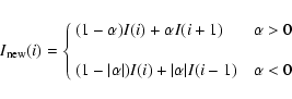
where
 |
(C.2) |
where
![\begin{figure}
\par\includegraphics[width=6.5cm,clip]{0143f28.eps}
\end{figure}](/articles/aa/full_html/2009/08/aa10143-08/img119.gif) |
Figure C.1:
A comparison of densities obtained from the Fe XII
|
| Open with DEXTER | |
The May 3 data set showed a number of compact features at different
temperatures however the Fe VIII comparison was compromised by the
blending of ![]() 185.21 and so the offset from the May 6 dataset was
preferred. Comparing several features, the offset between Fe XII
185.21 and so the offset from the May 6 dataset was
preferred. Comparing several features, the offset between Fe XII
![]() 186.88 and
186.88 and ![]() 196.64 was found to vary from 0.7 to 0.8 pixels -
we assume 0.75 here. For
196.64 was found to vary from 0.7 to 0.8 pixels -
we assume 0.75 here. For ![]() 195.12 and
195.12 and ![]() 203.72 the offset was 0.8 pixels, and for
203.72 the offset was 0.8 pixels, and for ![]() 192.39 and
192.39 and ![]() 195.12 it was 0.2 pixels.
195.12 it was 0.2 pixels.
Assuming that the grating tilt is linear, the offset for a given
wavelength is written as
| (C.3) |
where the offset is assumed to be zero at 195.12 Å. Computing the tilt from the four ratios and taking the average, we find m=-0.0792 pixels/Å.
To illustrate the consequence of the grating tilt on the derived densities, we consider a small brightening that appears at X-pixel 25 and Y-pixel 98 in the May 3 data set (see Fig. 17). Figure C.1 compares the densities derived from the two Fe XII density diagnostics in the vicinity of this brightening. The top panel shows the densities when no offsets are applied, the bottom panel shows the densities when the offsets have been applied. It is clearly seen that the peaks in density around pixels 96-100 do not coincide in the top panel, but do coincide in the bottom panel. The discrepancy in the top panel is striking and greater than would be expected simply from the sub-pixel spatial offsets derived for the lines. This is because taking the ratios of lines amplifies the effect of the intensity offsets.
Finally we note that there is some uncertainty in deriving the grating tilt due to the difficulty of co-aligning data at the sub-pixel level. This thus represents a possible systematic error in the derived density measurements that will be greatest for those lines with a large wavelength separation. It may affect density comparisons between ratios for small spatial features, but not the broad trends highlighted in Sect. 9.
References
- Aggarwal, K. M., & Keenan, F. P. 2004, A&A, 418, 371 [NASA ADS] [CrossRef] [EDP Sciences] (In the text)
- Aggarwal, K. M., & Keenan, F. P. 2005, A&A, 429, 1117 [NASA ADS] [CrossRef] [EDP Sciences] (In the text)
- Binello, A. M., Landi, E., Mason, H. E., Storey, P. J., & Brosius, J. W. 2001, A&A, 370, 1071 [NASA ADS] [CrossRef] [EDP Sciences] (In the text)
- Brickhouse, N. S., Raymond, J. C., & Smith, B. W. 1995, ApJS, 97, 551 [NASA ADS] [CrossRef] (In the text)
- Brooks, D. H., Warren, H. P., Ugarte-Urra, I., Matsuzaki, K., & Williams, D. R. 2007, PASJ, 59, S691 [NASA ADS] (In the text)
- Brosius, J. W., Davila, J. M., & Thomas, R. J. 1998, ApJS, 119, 255 [NASA ADS] [CrossRef] (In the text)
- Brown, C. M., Hara, H., Kamio, S., et al. 2007, PASJ, 59, S865 [NASA ADS] (In the text)
- Brown, C. M., Feldman, U., Seely, J. F., Korendyke, C. M., & Hara, H. 2008, ApJS, 176, 511 [NASA ADS] [CrossRef] (In the text)
- Chifor, C., Young, P. R., Isobe, H., et al. 2008, A&A, 481, L57 [NASA ADS] [CrossRef] [EDP Sciences] (In the text)
- Culhane, J. L., Harra, L. K., James, A. M., et al. 2007, Sol. Phys., 243, 19 [NASA ADS] [CrossRef] (In the text)
- Del Zanna, G., & Mason, H. E. 2003, A&A, 406, 1089 [NASA ADS] [CrossRef] [EDP Sciences]
- Del Zanna, G., & Mason, H. E. 2005, A&A, 433, 731 [NASA ADS] [CrossRef] [EDP Sciences] (In the text)
- Dere, K. P., & Mason, H. E. 1981, in Solar Active Regions, ed. F. Q. Orrall (Boulder: Colorado Associated Univ. Press), 129 (In the text)
- Dere, K. P., Landi, E., Mason, H. E., Monsignori-Fossi, B. C., & Young, P. R. 1997, A&AS, 125, 149 [CrossRef] [EDP Sciences] (In the text)
- Dere, K. P., Landi, E., Young, P. R., & Del Zanna, G. 2001, ApJS, 134, 331 [NASA ADS] [CrossRef] (In the text)
- Dere, K. P., Doschek, G. A., Mariska, J. T., et al. 2007, PASJ, 59, S721 (In the text)
- Doschek, G. A. 1984, ApJ, 279, 446 [NASA ADS] [CrossRef] (In the text)
- Doschek, G. A., Warren, H. P., Laming, J. M., et al. 1997, ApJ, 482, L109 [NASA ADS] [CrossRef]
- Doschek, G. A., Mariska, J. T., Warren, H. P., et al. 2007a, ApJ, 667, L109 [NASA ADS] [CrossRef] (In the text)
- Doschek, G. A., Mariska, J. T., Warren, H. P., et al. 2007b, PASJ, 59, S707 (In the text)
- Fawcett, B. C., & Mason, H. E. 1989, ADNDT, 43, 245 [NASA ADS] [CrossRef] (In the text)
- Feldman, U., Doschek, G. A., & Cohen, L. 1983 ApJ, 273, 822
- Flower, D. R. 1977, A&A, 54, 163 [NASA ADS] (In the text)
- Flower, D. R., & Nussbaumer, H. 1974, A&A, 31, 353 [NASA ADS] (In the text)
- Flower, D. R., & Pineau des Forêts, G. 1973, A&A, 24, 181 [NASA ADS] (In the text)
- Gupta, G. P., & Tayal, S. S. 1998, ApJ, 506, 464 [NASA ADS] [CrossRef] (In the text)
- Imada, S., Hara, H., Watanabe, T., et al. 2007, PASJ, 59, S793 (In the text)
- Keenan, F. P., Jess, D. B., Aggarwal, K. M., et al. 2007, MNRAS, 376, 205 [NASA ADS] [CrossRef] (In the text)
- Korendyke, C. M., Brown, C. M., Thomas, R. J., et al. 2006, Appl. Optics, 45, 8674 [NASA ADS] [CrossRef] (In the text)
- Jupén, C., Isler, R. C., & Träbert 1993, MNRAS, 264, 627 [NASA ADS] (In the text)
- Laming, J. M., Feldman, U., Schühle, U., et al. 1997, ApJ, 485, 911 [NASA ADS] [CrossRef] (In the text)
- Landi, E. 2002, A&A, 382, 1106 [NASA ADS] [CrossRef] [EDP Sciences] (In the text)
- Landi, E., Del Zanna, G., Young, P. R., et al. 2006, ApJS, 162, 261 [NASA ADS] [CrossRef]
- Landman, D. A. 1975, A&A, 43, 285 (In the text)
- Landman, D. A. 1978, ApJ, 220, 366 [NASA ADS] [CrossRef] (In the text)
- Mariska, J. T. 1992, The Solar Transition Region (CUP) (In the text)
- Mariska, J. T., Warren, H. P., Ugarte-Urra, et al. 2007, PASJ, 59, S713 (In the text)
- Neupert, W. M., Epstein, G. L., Thomas, R. J., & Thompson, W. T. 1992, Sol. Phys., 137, 87 [NASA ADS] [CrossRef] (In the text)
- Penn, M. J., & Kuhn, J. R. 1994, ApJ, 434, 807 [NASA ADS] [CrossRef] (In the text)
- Pike, C. D., & Harrison, R. A. 2000, A&A, 362, L21 [NASA ADS]
- Seely, J. F., Brown, C. M., Windt, D. L., Donguy, S., & Kjornrattanawanich, B. 2004, Appl. Opt., 43, 1463 [NASA ADS] [CrossRef] (In the text)
- Storey, P. J., Del Zanna, G., Mason, H. E., Zeippen, & C. J. 2005, A&A, 433, 717 [NASA ADS] [CrossRef] [EDP Sciences] (In the text)
- Tayal, S. S., Henry, R. J. W., Keenan, F. P., McCann, S. M., & Widing, K. G. 1991, ApJ, 369, 567 [NASA ADS] [CrossRef]
- Thompson, W. T., Haugan, S. V. H., & Young, P. R. 1998, CDS Software Note No. 46, version 2, available from http://solar.bnsc.rl.ac.uk/software/notes.shtml
- Watanabe, T., Hara, H., Culhane, J. L., et al. 2007, PASJ, 59, S669 (In the text)
- Young, P. R. 2004, A&A, 417, 785 [NASA ADS] [CrossRef] [EDP Sciences] (In the text)
- Young, P. R., & Esser, R. 1999a, Solar Wind Nine, AIP Conf. Proc., 471, 273
- Young, P. R., & Esser, R. 1999b, Space Sci. Rev., 87, 345 [NASA ADS] [CrossRef]
- Young, P. R., Landi, E., & Thomas, R. J. 1998, A&A, 329, 291 [NASA ADS] (In the text)
- Young, P. R., Klimchuk, J. A., & Mason, H. E. 1999, A&A, 350, 286
- Young, P. R., Del Zanna, G., Landi, E., et al. 2003, ApJS, 144, 135 [NASA ADS] [CrossRef] (In the text)
- Young, P. R., Del Zanna, G., Mason, H. E., et al. 2007a, PASJ, 59, S727 [NASA ADS] (In the text)
- Young, P. R., Del Zanna, G., Mason, H. E., et al. 2007b, PASJ, 59, S857 [NASA ADS] (In the text)
Footnotes
- ...
![[*]](/icons/foot_motif.gif)
- Present address: Space Science Division, Naval Research Laboratory, Washington, DC 20375, USA.
- ...Solarsoft
- Solarsoft is a set of integrated software libraries, databases, and system utilities that provide a common programming and data analysis environment for Solar Physics. It is available at http://www.lmsal.com/solarsoft.
- ... Markwardt
- http://astrog.physics.wisc.edu/~craigm/idl/idl.html
All Tables
Table 1: Transition information and CHIANTI wavelengths for the density diagnostics.
All Figures
| |
Figure 1:
Theoretical variation of emission line ratios versus electron
density for Fe XIII |
| Open with DEXTER | |
| In the text | |
| |
Figure 2:
The theoretical variation of the Fe XIII
|
| Open with DEXTER | |
| In the text | |
| |
Figure 3:
An example double-Gaussian fit to the Fe VIII |
| Open with DEXTER | |
| In the text | |
| |
Figure 4:
Spectrum from a single spatial pixel in the May 3 dataset
showing the wavelength window used to obtain the Fe XI
|
| Open with DEXTER | |
| In the text | |
| |
Figure 5:
The intensity ratio of S XI |
| Open with DEXTER | |
| In the text | |
| |
Figure 6:
Two example spectra from the May 3 data set showing the
emission lines neighbouring the strong Fe XII |
| Open with DEXTER | |
| In the text | |
| |
Figure 7:
An example double-Gaussian fit to Fe XIII |
| Open with DEXTER | |
| In the text | |
| |
Figure 8:
An example single Gaussian fit to the Fe XIII |
| Open with DEXTER | |
| In the text | |
| |
Figure 9:
An example fit to the feature at 203.8 Å that comprises
Fe XII |
| Open with DEXTER | |
| In the text | |
| |
Figure 10:
Theoretical variation of the Fe XIII
|
| Open with DEXTER | |
| In the text | |
| |
Figure 11:
Image of AR 10963 obtained in the Fe XII |
| Open with DEXTER | |
| In the text | |
| |
Figure 12:
The upper panel shows an image from the May 6 data set
obtained in the Fe XII |
| Open with DEXTER | |
| In the text | |
| |
Figure 13:
The same plot as Fig. 12 except for
Fe XIII. In the upper panel the image shown is from
Fe XIII |
| Open with DEXTER | |
| In the text | |
| |
Figure 14:
A comparison of densities derived from the Fe XII
|
| Open with DEXTER | |
| In the text | |
| |
Figure 15: Exactly analogous plot to Fig. 13, except the densities are derived using the Keenan et al. (2007) Fe XIII atomic model. |
| Open with DEXTER | |
| In the text | |
| |
Figure 16:
Context image of AR 10963 obtained on 2007 May 3 00:03 UT,
shortly before the raster analysed in
Sect. 7. The image was obtained by making a six
exposure raster with the 40
|
| Open with DEXTER | |
| In the text | |
| |
Figure 17:
The same plot as Fig. 12 except this time
for the May 3 data set. For the intensity curves from Fe XII
|
| Open with DEXTER | |
| In the text | |
| |
Figure 18:
The same plot as Fig. 13 except this time
for the May 3 data set. For the intensity curve from Fe XIII
|
| Open with DEXTER | |
| In the text | |
| |
Figure 19:
A comparison of densities derived from the Fe XII
|
| Open with DEXTER | |
| In the text | |
| |
Figure 20: Exactly analogous plot to Fig. 18, except the Fe XIII densities are derived using the Keenan et al. (2007) atomic model. |
| Open with DEXTER | |
| In the text | |
| |
Figure 21:
Comparisons of line widths and velocities for the density
diagnostic lines of Fe XII and Fe XIII from the May 6
and May 3 data sets. For Fe XII, |
| Open with DEXTER | |
| In the text | |
| |
Figure 22:
A comparison of the measured variation of the Fe XII |
| Open with DEXTER | |
| In the text | |
| |
Figure 23:
A comparison of the measured variation of the Fe XIII |
| Open with DEXTER | |
| In the text | |
| |
Figure 24:
A comparison of densities derived from
Fe XII |
| Open with DEXTER | |
| In the text | |
| |
Figure A.1:
A comparison of the full widths at half maxima (FWHM) of
Gaussian fits to the Fe XII |
| Open with DEXTER | |
| In the text | |
| |
Figure A.2:
A comparison of the measured variation of the Fe XII
|
| Open with DEXTER | |
| In the text | |
| |
Figure B.1:
Comparison of measured Fe XII |
| Open with DEXTER | |
| In the text | |
| |
Figure C.1:
A comparison of densities obtained from the Fe XII
|
| Open with DEXTER | |
| In the text | |
Copyright ESO 2009
Current usage metrics show cumulative count of Article Views (full-text article views including HTML views, PDF and ePub downloads, according to the available data) and Abstracts Views on Vision4Press platform.
Data correspond to usage on the plateform after 2015. The current usage metrics is available 48-96 hours after online publication and is updated daily on week days.
Initial download of the metrics may take a while.