


| Issue |
A&A
Volume 712, August 2026
|
|
|---|---|---|
| Article Number | A9 | |
| Number of page(s) | 10 | |
| Section | Planets, planetary systems, and small bodies | |
| DOI | https://doi.org/10.1051/0004-6361/202660649 | |
| Published online | 30 July 2026 | |
Spatial profiles and scale lengths of nickel, iron, and CN on the interstellar comet 3I/ATLAS
1
Università degli Studi di Padova (UNIPD), Dipartimento di Fisica e Astronomia “G. Galilei”,
Via F. Marzolo 8,
35131
Padova,
Italy
2
Istituto Nazionale di Astrofisica (INAF) – Osservatorio Astronomico di Padova,
Vicolo dell’Osservatorio 5,
35122
Padova,
Italy
3
Koyama Space Science Institute, Kyoto Sangyo University, Kamigamo Motoyama, Kita-ku, Kyoto,
Kyoto
603-8555,
Japan
4
Division of Science, Kyoto Sangyo University, Kamigamo Motoyama, Kita-ku, Kyoto,
Kyoto
603-8555,
Japan
5
Photocross Co., Ltd., Bldg. D, Iwakura-Chuzaichi-cho, Sakyo-ku,
Kyoto
606-0021,
Japan
6
Stazione Astronomica di Sozzago, Cascina Guascona,
28060
Sozzago (Novara),
Italy
★ Corresponding author: This email address is being protected from spambots. You need JavaScript enabled to view it.
Received:
27
April
2026
Accepted:
18
June
2026
Abstract
Context. Interstellar objects are the relics of planetary formation of extrasolar systems. They represent a unique opportunity to study insights of planetary formations around other stars. Since the discovery of 1I/‘Oumuamua in 2017, only two more interstellar objects have been found. 3I/ATLAS is the third, and its cometary nature was confirmed by early observations.
Aims. Long-slit spectra of comet 3I/ATLAS were obtained with the 1.22 m telescope at the Asiago Astrophysical Observatory. The 7’ slit provided sufficient spatial coverage through the coma to investigate the release of atomic and molecular species. We provide the first extensive spatial-distribution study of species in the coma of the interstellar comet 3I/ATLAS, with a total coverage of up to 2.8·105 km. Such spatial information has not previously been reported in the literature. We analysed the Fe I, Ni I, and CN emission features observed at 2.17 AU.
Methods. We extracted the two-dimensional long-slit spectrum and performed the wavelength and flux calibration. From the resulting spectrum, we analysed the cometary emission line spatial distribution and the production rates of the parent molecules through a Haser modelling approach.
Results. Several neutral iron and nickel lines were detected together with the CN B-X (0–0) band. Production rates of CN and C3 and 3σ NH upper limits were computed as well. We obtained the scale length of nickel, ld(Ni) = 8.26−1.48+2.12 105 km, and iron, ld(Fe) = 2.48−0.42+0.57 105 km. These results imply a slower outflow velocity with respect to Solar System comet values. The relative abundance was found: Ni/Fe = 0.20 ± 0.11. For CN, the obtained scale length is in agreement with typical values adopted for Solar System comets, but the CN parent scale length of lp(CN) = 4.52−0.03+0.03 104 km we found is notably shorter than the usual values assumed or fitted for the CN parent in the literature.
Conclusions. The iron and nickel scale lengths we computed suggest that they originate from a short-lived parent, with no indication of an extended source in the coma. The lifetime of atoms are compatible with photoionisation under active Sun conditions. Our analysis of the CN spatial profile provides the first evidence that CN production in an interstellar comet may not follow the standard behaviour observed in Solar System comets. Our results indicate that CN in 3I likely originates from a combination of known parent molecules together with an additional short-lived component or, alternatively, from a parent species with an outflow velocity significantly lower than typically inferred for Solar System comets.
Key words: comets: general / comets: individual: 3I/ATLAS
© The Authors 2026
 Open Access article, published by EDP Sciences, under the terms of the Creative Commons Attribution License (https://creativecommons.org/licenses/by/4.0), which permits unrestricted use, distribution, and reproduction in any medium, provided the original work is properly cited.
This article is published in open access under the Subscribe to Open model. This email address is being protected from spambots. You need JavaScript enabled to view it. to support open access publication.
1 Introduction
Interstellar objects offer a unique window into the formation environments of planetary systems beyond our own, and analysis of their compositions may provide critical information about planetary formation processes that differ from what is observed in our neighbourhood. The first two interstellar objects discovered are radically different from each other. The first, 1I/‘Oumuamua, behaves essentially as an asteroid. It shows no detectable activity and exhibits an unusually high aspect ratio (Meech et al. 2017; Micheli et al. 2018), although its trajectory has revealed non-gravitational accelerations that were tentatively linked to CO outgassing (Seligman et al. 2021). In contrast, 2I/Borisov is a comet in all respects, with properties closely resembling those of Solar System comets (Opitom et al. 2019; Jewitt & Luu 2019; Mazzotta Epifani et al. 2021; Cremonese et al. 2020; Fitzsimmons et al. 2019). On 1 July 2025, a third interstellar object was identified (Denneau et al. 2025). Early observations revealed the presence of a coma, establishing it as the second confirmed interstellar comet after 2I/Borisov. Precovery images from the Transiting Exoplanet Survey Satellite (TESS) indicate that activity may have begun almost at a heliocentric distance of approximately 6 AU (Feinstein et al. 2025). Several observing campaigns have begun to obtain an initial characterisation of this new visitor. Early observations at rh ~ 4 AU revealed a redder slope with respect to 2I/Borisov, consistent with D-type asteroids (de la Fuente Marcos et al. 2025; Seligman et al. 2025; Puzia et al. 2025; Bolin et al. 2025; Xing et al. 2025; Opitom et al. 2025) and in some cases comparable to that of Solar System comets (Santana-Ros et al. 2025). At this point, no emission bands in the visible range have been detected, and there are only upper limits for CN and OH (Alvarez-Candal et al. 2025).
In the near-infrared (NIR), the spectrum becomes flatter, and modelling suggests a grain distribution that differs from Solar System comets (Kareta et al. 2025) and the presence of water ice grains in the coma (Yang et al. 2025; Xing et al. 2025). Observations with the Hubble Space Telescope at 3.8 AU pre-perihelion revealed that the nucleus radius should not be larger than about 2.8 km and not less than ~0.22 km, assuming a CO-driven activity (Jewitt et al. 2025). Observations with the James Webb Space Telescope (JWST) at 3.32 AU report a CO2-dominated coma and detectable H2O, CO, water ice, and dust and a tentative identification of the OCS molecule. Cordiner et al. (2025) found a high CO2/H2O ratio, suggesting an intrinsically CO2-rich nucleus or suppressed water sublimation (Cordiner et al. 2025). More recent optical spectroscopic observations have detected the onset of CN activity as far out as 3.2 AU (Salazar Manzano et al. 2025; Lazzarin et al. 2026) as well as strong carbon-chain depletion. This depletion is no longer evident in the post-perihelion data, while marked depletion of NH2 (Kawakita et al. 2026) and NH have emerged (Jehin et al. 2025b). At radio and submillimetre wavelengths, pre-perihelion observations have revealed lines of HCN and CH3OH with ratios of HCN/H2O and CN/HCN compatible with Solar System comet values (Coulson et al. 2026) and CH3OH/HCN compatible with the upper limits of Solar System comet measurements (Roth et al. 2026). 3I revealed an extremely low sulphur-to-carbon abundance and an unusually low gas expansion velocity, which is compatible with the presence of heavy molecules such as CO2 in the inner coma (Biver et al. 2026). Iron and nickel lines in 3I have been observed preperihelion (Rahatgaonkar et al. 2025; Hutsemékers et al. 2026). Rahatgaonkar et al. (2025) observed unusually strong Ni I lines and the CN violet band near 3883 Å but no Fe I nor C2, C3, NH2, or [O I] from rh ~ 4.4–2.85 AU. They suggest that the steep rise of nickel and CN production towards the Sun is due to the release from low-energy dust-driven processes, such as photo-desorption or thermolysis of metal-bearing compounds such as iron- and nickel-carbonyls, rather than from sublimation from conventional metallic or sulphide phases. Hutsemékers et al. (2026) report strong Ni I emission in 3I/ATLAS at all observed distances and Fe I only closer to the Sun, revealing an initially extreme Ni/Fe ratio that later evolved to values typical of Solar System comets. In this context, the authors suggest that high metal production rates and the change in Ni/Fe ratio are best explained by the release of nickel and iron from volatile carbonyl compounds (Ni(CO4, Fe(CO)5), rather than by direct sublimation of refractory minerals.
In this study, we report the detection of iron and nickel lines as well as the CN B-X (0–0) and C3 A-X bands in the spectrum of comet 3I/ATLAS. The comet was observed at rh = 2.17 AU post-perihelion with the 1.22m Galileo telescope at the Asiago Astrophysical Observatory. The adopted setup allows for high spatial coverage of 3I’s coma up to a nucleocentric distance of ρ ~ 2.8 · 105 km. The spatial distribution of the molecules in 3I’s coma has not been investigated in detail to date, and our observations offer the first basis for a new characterisation of the spatial distribution of the observed species. The scale lengths of Ni, Fe, and CN in the interstellar comet 3I/ATLAS were derived from their spatial profiles, allowing us to discuss the nature of their parent molecules.
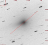 |
Fig. 1 Frame of 3I/ATLAS at 600s taken in the sloan r filter from the same observing session of spectroscopy with the 0.67/0.92 m Schmidt telescope (INAF-OAPD), Asiago. The orientation of the long-slit is shown. |
2 Observations and data reduction
Spectra of 3I/ATLAS were obtained with the 1.22m Galileo telescope at the Asiago Astrophysical Observatory (MPC-IAU code: 043) when the comet was at rh = 2.17 AU, with the 1200 lines/mm grating, which has dispersion of 0.6 Å/px. The grating angle was adjusted to access the UV configuration, which covers the 3300–4570 Å spectral range with a resolving power of R ~ 2000. The effective area of the charge-coupled device (CCD) is 435 × 2034 pixels, and each pixel has a size of 13.5 × 13.5 micron and a pixel scale of 1.00”/px. The spectrograph long-slit aperture has an effective length of 7.25′ and a width of 2.56” on the focal plane. The slit was oriented along the parallactic angle to avoid any differential flux loss due to atmospheric diffraction. In Fig. 1, the slit orientation during the observing run is shown. Comet 3I was observed in the context of a cometary monitoring project conducted at the Asiago Astrophysical Observatory1. Three spectra of 3I/ATLAS were obtained, each with an exposure time of 1200 s. Additional observations included a spectrum of the spectrophotometric standard star HR 7001 for flux calibration and the solar-analog star 16 Cygni B, which was used to characterise the contribution of reflected sunlight from cometary dust. We used standard Image Reduction and Analysis Facility (IRAF) routines (Tody 1986) for bias subtraction and flat-field correction. Wavelength calibration was performed using He-Fe-Ar hollow-cathode lamp spectra acquired immediately before and after the comet’s observations. The three comet exposures were co-added to increase the signal-to-noise ratio. Flux calibration was derived by comparing the observed HR 7001 spectrum with the corresponding ESO reference spectrum. A slit-loss correction factor was computed from the calibration star observations and applied to the final flux-calibrated comet spectrum to account for light losses at the slit. In order to remove the sky background, a median sky spectrum was extracted by combining two 20-pixel windows located at the bottom and top edges of the slit. We subtracted the final median sky spectrum from each row of the two-dimensional comet spectrum. The curvature of the sky lines was already corrected along with the wavelength calibration by the IRAF routine transform, a procedure which straightens the CCD rows while applying the wavelength solution. This minimised any residual flux from the sky lines. The approach of extracting a sky spectrum from the same frame as the target avoids the strong temporal variability of the night sky, which affects frames taken at different times, and therefore significantly improves the sky subtraction. Because the CN band emission extended across the entire slit, its wavelength region was excluded from the sky spectrum before subtracting it from the comet spectrum. Finally, the solar-analog spectrum was used to remove the solar features, and a polynomial fit was applied to subtract the residual dust continuum emission.
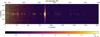 |
Fig. 2 Two-dimensional co-added spectrum of 3I/ATLAS with the sky and dust continuum removed. |
3 Data analysis and methodology
The two-dimensional co-added frame of 3I (Fig. 2) shows several iron and nickel lines (Table A.2), the CN band near 3883 Å, and the C3 band at 3920–4100 Å. The slit was centred on the nucleus, providing a spatial coverage of about 284 000 km in both directions. The two-dimensional frame was analysed to characterise the spatial distribution of atomic and molecular emissions in the coma. The derived one-dimensional summed spectrum (Fig. 3) was used to extract the integrated flux of each emission line or band. In the case of the C3 band, the received signal was not sufficient to allow for spatial distribution analysis, so the production rate was computed from the summed-up one-dimensional spectrum. The atomic and molecular spatial profiles were analysed within a Haser-model framework. The Haser model (Haser 1957) assumes a spherically symmetric coma, where parent molecules are uniformly emitted from the nucleus at a constant expansion velocity, ![Mathematical equation: $\[0.85 ~\mathrm{r}_{h}^{-0.5}\]$](/articles/aa/full_html/2026/08/aa60649-26/aa60649-26-eq4.png) km s−1 (Cochran & Schleicher 1993) and are subsequently photodissociated by solar radiation into daughter species. This model assumes that (a) collisions in the inner coma are negligible, (b) the medium is optically thin, and (c) the velocity kick imparted to the daughter species is not taken into account. The Haser model provides the simplest description of cometary comae and is widely used to interpret the observed atomic and molecular spatial profiles. Moreover, it allows one to investigate parent-daughter relationships, derive molecular and atomic production rates, and compare different comets (A’Hearn et al. 1995; Fink 2009; Langland-Shula & Smith 2011; Cochran et al. 2012; Munaretto et al. 2026).
km s−1 (Cochran & Schleicher 1993) and are subsequently photodissociated by solar radiation into daughter species. This model assumes that (a) collisions in the inner coma are negligible, (b) the medium is optically thin, and (c) the velocity kick imparted to the daughter species is not taken into account. The Haser model provides the simplest description of cometary comae and is widely used to interpret the observed atomic and molecular spatial profiles. Moreover, it allows one to investigate parent-daughter relationships, derive molecular and atomic production rates, and compare different comets (A’Hearn et al. 1995; Fink 2009; Langland-Shula & Smith 2011; Cochran et al. 2012; Munaretto et al. 2026).
3.1 Spatial distribution of iron and nickel
Concerning the analysis of spatial profiles, we selected the brightest individual iron and nickel lines, namely, the 3525 Å line for nickel and the 3720 Å line for iron. Their integrated flux was derived by averaging the flux at each nucleocentric distance in the two slit directions. As the 3720 Å iron line did not provide an S/N comparable to that of the 3525 Å nickel line, multiple iron lines (listed in Table A.1) were co-added to enhance the signal. The scale lengths of nickel and iron were derived following the procedure described in Guzik & Drahus (2021): their spatial distributions were modelled with a Haser profile, assuming that both species originate from a short-lived parent released near the nucleus, imposing lp < 1000 km. To constrain the Haser scale lengths, the observed radial profile was normalised to its maximum value to fit only the shape of the distribution. In this normalised framework, the production rate appears as a multiplicative constant, which was treated as a free scaling parameter (A). Model parameters were estimated using a Bayesian approach implemented with the affine-invariant ensemble sampler in emcee (Foreman-Mackey et al. 2013), which performs Markov chain Monte Carlo (MCMC) sampling of the posterior distribution. The best-fit parameters and uncertainties from an initial least-square fit were used to define informative Gaussian priors for the MCMC initialisation. Given that iron and nickel are also commonly described by a 1/ρ profile (Manfroid et al. 2021), we also considered it in our analysis (Fig. 6).
The iron and nickel emission lines were detected along the slit up to a nucleocentric distance of 101 428 km, beyond which the signal-to-noise ratio became too low for reliable tracking. This represents a larger spatial coverage than previously reported in the literature. The shortest nucleocentric radii were affected by the seeing, which varied along the night among 2.5” and 5”. Considering these variations, the seeing was included as a fitted parameter in our procedure, in terms of a Gaussian smoothing applied to the Haser model. Given the projected dimension of the seeing (~6000 km) and the widely accepted hypothesis that iron and nickel atoms are produced in the immediate vicinity of the nucleus (Manfroid et al. 2021), we did not assign any physical meaning to the inferred parent scale lengths. The fitted parameters are reported in Table 1. The fitted seeing value varies between species, and in particular it tends to be smaller for iron and nickel than for CN. Although some wavelength-dependence or instrumental effects could contribute to this behaviour, in the case of iron and nickel, the model also struggles to disentangle the parent scale length from the seeing, which likely biases the fitted seeing disk. This may lead to an underestimation of the seeing during the fit.
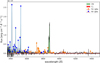 |
Fig. 3 One-dimensional co-added frame of 3I/ATLAS. The blue and orange delta functions indicate the nickel and iron transitions for which the g factors were computed. |
3.2 Iron and nickel abundances
Several iron and nickel lines were identified using the FlorPy fluorescence model. Of these, 11 Ni and 9 Fe transitions exhibited an adequate signal and negligible blending, making them suitable for Gaussian fitting. These lines are listed and described in Table A.2, and a representative plot is shown in Fig. 3. The FlorPy code (Bromley et al. 2021) performs a fluorescence equilibrium computation, assuming a collision-less and optically thin coma. This model was used to produce the population and fluorescence efficiency for all atomic lines and transitions reported in the Atomic Spectra Database of the National Institute of Standards and Technology2. With heliocentric and geocentric distances and velocities as inputs, FlorPy takes into account the solar irradiance at the comet’s position and relative velocity effects on the computed populations. It uses a composite solar spectrum (fully described in Bromley et al. 2021) to evaluate the radiation field at the comet’s position and with respect to the comet’s velocity. Since the observations were carried out during a phase of solar maximum, we examined the variability of the solar flux across our spectral range to assess how much this effect could influence the resulting g factors. According to Lean (2001), the solar variability from 200 to 1000 nm is of the order of a few tenths of a percent. For this reason, a 20% uncertainty was added in quadrature to the g-factor estimation. The relative g factor was associated with any observed line flux. With the obtained scale length, the total number of atoms in the aperture could be obtained by
![Mathematical equation: $\[n_d=\frac{F_{i j} 4 \pi \Delta^2}{g_{i j}},\]$](/articles/aa/full_html/2026/08/aa60649-26/aa60649-26-eq5.png) (1)
(1)
where Fij is the integrated flux of the single line (erg s−1 cm−2) and gij is the fluorescence efficiency of the same line computed through FlorPy (erg s−1). Each Fij value was determined by fitting the corresponding line with a Gaussian profile using a Levenberg–Marquardt minimiser (Press et al. 1992) implemented through the scipy library curve_fit function at the known line positions (Virtanen et al. 2020). The results of the Gaussian fit for any line are visible in Fig. A.1. The uncertainty of each integrated flux was obtained by combining the covariance-matrix errors on the Gaussian amplitude and width with the standard deviation of nearby continuum regions. The uncertainties on gij were provided by the FlorPy computation. From the total number of atoms, the production rate Q (atoms s−1) was computed as
![Mathematical equation: $\[Q=\frac{n_d ~v_{\text {out}}}{\mathrm{HF} ~l_d},\]$](/articles/aa/full_html/2026/08/aa60649-26/aa60649-26-eq6.png) (2)
(2)
where ‘HF’ is the Haser fraction (A’Hearn et al. 1995; Fink & Hicks 1996), which is needed to obtain the total number of atoms in the coma from the number of atoms inside the aperture; vout is the outflow velocity, assumed to be ![Mathematical equation: $\[0.85 ~\mathrm{r}_{h}^{-0.5}\]$](/articles/aa/full_html/2026/08/aa60649-26/aa60649-26-eq7.png) km s−1 (Cochran & Schleicher 1993); and ld (km) is the daughter scale length computed by fitting the spatial profile. Finally, the nickel and iron abundance ratio was computed with the following expression: Ni/Fe = log10(QNi/QFe).
km s−1 (Cochran & Schleicher 1993); and ld (km) is the daughter scale length computed by fitting the spatial profile. Finally, the nickel and iron abundance ratio was computed with the following expression: Ni/Fe = log10(QNi/QFe).
3.3 Spatial distribution of CN
For CN, the most straightforward approach was to use the band-integrated g factor computed by Schleicher (2010) and to fit Q, lp, and ld simultaneously, given that the band is largely unresolved. In this case, the flux measurements were not normalised. As before, an initial deterministic fit using the scipy curve_fit routine was performed to determine the priors for the subsequent MCMC analysis. For CN, the parent scale length is significantly larger than the seeing disk, so both the parent and daughter scale lengths are physically meaningful. To evaluate the influence of the seeing parameter on the retrieved production rate, a Q-curve analysis approach was used (see Disanti & Mumma (2008) for a review). In this method, the production rate, Q, is computed independently at each nucleocentric radius, thus allowing for the identification of the inner region size where the computed Q is highly sensitive to seeing. The innermost radii are affected because atmospheric seeing smooths the central divergence of the Haser profile and redistributes flux outside the aperture, preventing a direct comparison with the model. The resulting Q-curve indicated the radii at which the production rate is not reliably constrained. Excluding the first six points and fitting a straight line to the remaining values yielded an apertureindependent production rate. This result is consistent with the value obtained from the MCMC fit. To compute the C3 production rate and NH upper limit, a Fink & Hicks (1996) approach was used (Eq. (1)) with the scale lengths and g factors used in A’Hearn et al. (1995) and Cochran & Schleicher (1993).
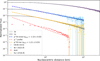 |
Fig. 4 Spatial distribution of iron, nickel, and the CN band. The solid line is the resulting MCMC best fit. The dashed lines are the best fit for the ρa profile. For comparison, the dust profile is also shown. The dust continuum used was 440–450 nm. |
Best–fit parameters for Ni I, Fe I, and CN.
4 Results
4.1 Iron and nickel
The strongest iron feature (3720 Å) has a measured integrated flux of (5.76 ± 0.37) 10−14 erg cm−2 s−1, and the strongest Ni line (3525 Å) was detected with an integrated flux of (2.25 ± 0.07) 10−13 erg cm−2 s−1. The radial distribution of iron and nickel was traced along the slit orientation and fitted with a Haser model. The same procedure was also applied to the CN band, resulting in an integrated flux of (7.94 ± 0.01) 10−13 erg cm−2 s−1. The results of the fit are shown in Fig. 4 and reported in Table 1. Using Eq. (1), the fluorescence equilibrium outputs from FlorPy were used to compute the total number of iron and nickel atoms within the aperture, with the following results: (1.22 ± 0.38) 1028 atoms for Fe I and (2.50 ± 0.56) 1028 atoms for Ni I. The production rates of nickel and iron were computed through Eq. (2), resulting in QNi = (1.13 ± 0.18) 1024 atoms s−1 and QFe = (7.06 ± 1.11) 1023 atoms s−1. The corresponding Ni/Fe abundance ratio derived from these values is log10(QNi/QFe) = 0.20 ± 0.11, which is in agreement with the value reported by Zhao et al. (2026). We compared the measured profile with the typically assumed ρ−1 distribution (Fig. 6). This fit produced a slightly steeper slope for both iron and nickel spatial distributions: −1.10 ± 0.02 for nickel and −1.21 ± 0.03 for iron.
4.2 CN spatial distribution and molecules production rate
For the CN production rate, the result of the MCMC fit produced QCN = ![Mathematical equation: $\[1.85_{-0.01}^{+0.01}\]$](/articles/aa/full_html/2026/08/aa60649-26/aa60649-26-eq28.png) 1025 molec s−1 at rh = 2.17 AU and scale lengths of ld =
1025 molec s−1 at rh = 2.17 AU and scale lengths of ld = ![Mathematical equation: $\[4.52_{-0.03}^{+0.03}\]$](/articles/aa/full_html/2026/08/aa60649-26/aa60649-26-eq29.png) 104 km and lp =
104 km and lp = ![Mathematical equation: $\[9.60_{-0.21}^{+0.21}\]$](/articles/aa/full_html/2026/08/aa60649-26/aa60649-26-eq30.png) 105 km, assuming an outflow velocity of
105 km, assuming an outflow velocity of ![Mathematical equation: $\[0.85 ~\mathrm{r}_{h}^{-0.5}\]$](/articles/aa/full_html/2026/08/aa60649-26/aa60649-26-eq31.png) km s−1 (Cochran & Schleicher 1993). The fitted QCN from Q-curve analysis is 1.89 ± 0.01 1025 molec s−1. For C3 the computed production rate is QC3 = 3.65 ± 0.03 1024 molec s−1, which leads to a logarithmic ratio with CN of log10(QC3/QCN) = 0.71. The computed 3σ upper limit for NH is <1.45 1025 molecules s−1, and the relative ratio to CN is −0.12.
km s−1 (Cochran & Schleicher 1993). The fitted QCN from Q-curve analysis is 1.89 ± 0.01 1025 molec s−1. For C3 the computed production rate is QC3 = 3.65 ± 0.03 1024 molec s−1, which leads to a logarithmic ratio with CN of log10(QC3/QCN) = 0.71. The computed 3σ upper limit for NH is <1.45 1025 molecules s−1, and the relative ratio to CN is −0.12.
5 Discussion
5.1 Iron and nickel
The observation of iron and nickel lines up to 3 AU is something that has also been observed in Solar System comets (Manfroid et al. 2021). This is a phenomenon that does not have a definitive explanation yet. Indeed, the first time that metal lines, such as iron, nickel, copper, and cobalt, were observed was in sungrazing comets such as Ikeya-Seki (Slaughter 1969) and the Great Comet of 1882 (Copeland & Lohse 1882), both below 0.01 AU. When a comet is in such proximity to the Sun, a reasonable explanation for metal lines is the direct sublimation from refractory compounds such as silicate, sulfide, and metal grains. This explanation is also coherent with the findings of in situ missions such as Giotto, Stardust, and Rosetta (Jessberger et al. 1988; Stenzel et al. 2017; Zolensky et al. 2006).
When comets exhibit metal lines far from the Sun, a different mechanism is needed since temperatures are too low to allow direct metal sublimation. Both 2I/Borisov and 3I/ATLAS have shown iron and nickel lines far beyond the distance where the sublimation of silicate, metal, and sulfide compounds is reasonable (Guzik et al. 2020; Opitom et al. 2021; Hutsemékers et al. 2021; Rahatgaonkar et al. 2025). The most credible explanation for how this happens is currently the one of Manfroid et al. (2021), which suggests the presence of complexes such as [Fe(PAH)]+ and carbonyls such as Fe(CO)5 and Ni(CO)4, already hypothesised by Klotz et al. (1996), that sublimate at high heliocentric distances. This interpretation is based on earlier work (e.g. Klotz et al. 1996) and on the sublimation behaviour of Fe(CO)5 and Ni(CO)4. Their sublimation rates make their presence in cometary comae plausible up to 3 AU and explains the observed relative Ni/Fe abundance. The photodissociation pathways required to release atomic Fe and Ni from these molecules were later explored in detail by Bromley et al. (2021), who constructed a framework relying on several assumptions, including that each absorbed UV photon removes a single CO molecule and that all intermediate fragments share the same absorption cross-section as the parent molecule. Under these conditions, sequential CO loss would fully strip the carbonyls within ~120–150 km of the nucleus. While this mechanism is plausible (Cole-Filipiak et al. 2021), it depends on unverified cross-sections for intermediate complexes, and laboratory studies show that prompt atomic emission from carbonyl dissociation is weak or absent (Ribar et al. 2015). Metal carbonyls therefore remain a possible but still unconfirmed source of cometary Fe and Ni atoms, and only further laboratory studies have the capability to confirm it. In this context, the analysis of the spatial distributions of iron and nickel plays an important role in constraining the mechanisms responsible for their emission. Our data reveal that the spatial profile of both atoms is correctly reproduced by a short-lived parent. No evidence was found for any extended-source production. To further assess this point, the usual 1000 km upper limit on lp was removed, and the parameter was allowed to vary freely over a wider range. The seeing was estimated from the standard-star spectrum and adopted as a lower bound; we note that this value does not include additional broadening from telescope-tracking errors, which are relevant during comet observations. All the results are reported in Table 1. If the lp is left free to vary, its value adjusts to values that are still below 1000 km, which is within the seeing disk. Beyond this region, the model requires only the daughter distribution, suggesting that any parent species must be released within the 4” seeing disk.
To assess consistency with published photoionisation values at 1 AU under active-Sun conditions, the lifetimes of 5.35 · 105 s for nickel and 5.13 · 104 s for iron from Huebner & Mukherjee (2015) were converted to scale lengths at 2.17 AU (Eq. (3)). Agreement with these values was explored by adopting different values for the gas outflow velocity. Figure 5 shows the computed values for the iron and nickel scale lengths. Using the outflow velocity derived for HCN by Biver et al. (2026) (0.32–0.43 km s−1 at 1.37 AU), we obtained a corresponding range of parent scale lengths. The values inferred from ALMA observations (Roth et al. 2026) fall near the midpoint of the Biver et al. (2026) confidence interval. For comparison, we also computed the scale lengths using the standard ![Mathematical equation: $\[0.85 ~r_{h}^{-0.5}\]$](/articles/aa/full_html/2026/08/aa60649-26/aa60649-26-eq33.png) km s−1 outflow velocity law. This comparison highlights how strongly the assumed outflow velocity, and in particular its heliocentric scaling, affects the resulting parent scale lengths. The
km s−1 outflow velocity law. This comparison highlights how strongly the assumed outflow velocity, and in particular its heliocentric scaling, affects the resulting parent scale lengths. The ![Mathematical equation: $\[\mathrm{r}_{h}^{-0.5}\]$](/articles/aa/full_html/2026/08/aa60649-26/aa60649-26-eq34.png) scaling is derived from observations of Solar System comets, and its applicability to the present case is not guaranteed. Consequently, the conversion of lifetimes and scale lengths from 1 AU to the observed heliocentric distance may introduce a systematic bias if the true velocity law deviates from this assumption. In line with this matter, the 1/ρ profile fit (Fig. 4) showing steeper slopes may be indicative of a different radial behaviour. In particular, a steeper slope may suggest a lower density in the outer coma. This interpretation is consistent with the slow inner coma expansion velocity expected in the presence of heavy molecules, as in Biver et al. (2026). In Fig. 4 the dust profile is also shown for comparison, which appears steeper with respect to the iron and nickel profiles. Finally, our Ni/Fe ratio agrees with the modelling of the Ni/Fe ratio expected from carbonyls, as explained in Hutsemékers et al. (2026).
scaling is derived from observations of Solar System comets, and its applicability to the present case is not guaranteed. Consequently, the conversion of lifetimes and scale lengths from 1 AU to the observed heliocentric distance may introduce a systematic bias if the true velocity law deviates from this assumption. In line with this matter, the 1/ρ profile fit (Fig. 4) showing steeper slopes may be indicative of a different radial behaviour. In particular, a steeper slope may suggest a lower density in the outer coma. This interpretation is consistent with the slow inner coma expansion velocity expected in the presence of heavy molecules, as in Biver et al. (2026). In Fig. 4 the dust profile is also shown for comparison, which appears steeper with respect to the iron and nickel profiles. Finally, our Ni/Fe ratio agrees with the modelling of the Ni/Fe ratio expected from carbonyls, as explained in Hutsemékers et al. (2026).
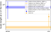 |
Fig. 5 Comparison between the computed iron and nickel parent scale lengths (with 3σ error bars) and the photoionisation values from Huebner & Mukherjee (2015). Different outflow velocities are shown: the highlighted region corresponds to the range of parent scale lengths obtained using the HCN outflow velocity from Biver et al. (2026); the segmented lines indicate the HCN scale lengths derived from ALMA observations (Roth et al. 2026); and the solid lines represent the scale lengths computed using the standard |
![Mathematical equation: $\[0.85 ~r_{h}^{-0.5}\]$](/articles/aa/full_html/2026/08/aa60649-26/aa60649-26-eq32.png)
5.2 Ni/Fe and NH depletion
Another relevant point is the potential correlations between carbon-chain depletion, NH depletion, and an enhanced Ni/Fe abundance ratio (Hutsemékers et al. 2021). This is particularly relevant in light of the variations observed in 3I/ATLAS, both in its Ni/Fe ratio and in its degree of carbon-chain depletion before and after perihelion. It is also notable that, although the carbon depletion disappears in the post-perihelion data, no trace of NH2 or NH has ever been detected on 3I at any point along its orbit (Jehin et al. 2025a). To test whether a such correlation holds, we evaluated and correlated the 3σ upper limits of NH with Ni/Fe abundance (Fig. 6). In the spectral range of the NH band, there are two moderately strong Ni lines. The fluorescence model was used to retrieve the flux of these lines and remove the contamination from the NH wavelength region. The resulting abundance ratio is log10(QNH/QCN) < 0.36. This value indicates a high NH depletion. In Fig. 6, 3I abundances are compared to 2I/Borisov values. The figure shows that they tend to align with the correlations suggested by Hutsemékers et al. (2021). A comparison with Solar System NH abundance is shown in Fig. A.2. In particular, the measured NH abundance of 3I is compared with the dataset of Cochran et al. (2012).
Photodissociation rates of proposed CN parent molecules at 1 AU.
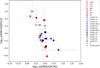 |
Fig. 6 Reproduction of the plot of correlation between Q(Ni)/Q(Fe) and Q(NH)/Q(CN) from Hutsemékers et al. (2021) but including the results computed here. |
5.3 CN
The fitted CN parent scale length revealed an unexpected difference compared to Solar System comets. Our parent scale length of lp = (![Mathematical equation: $\[4.52_{-0.03}^{+0.03}\]$](/articles/aa/full_html/2026/08/aa60649-26/aa60649-26-eq35.png) ) 104 km remains significantly smaller than expected compared to both standard
) 104 km remains significantly smaller than expected compared to both standard ![Mathematical equation: $\[\mathrm{r}_{h}^{2}\]$](/articles/aa/full_html/2026/08/aa60649-26/aa60649-26-eq36.png) scaling (Cochran & Schleicher 1993) and, for example, the scaling presented in Langland-Shula & Smith (2011). The fitted scale length from Table 10 of Langland-Shula & Smith (2011), lp(CN) = (3.0 ± 0.5)· 104 km at 1 AU, and their fitted rh scaling law from Table 9,
scaling (Cochran & Schleicher 1993) and, for example, the scaling presented in Langland-Shula & Smith (2011). The fitted scale length from Table 10 of Langland-Shula & Smith (2011), lp(CN) = (3.0 ± 0.5)· 104 km at 1 AU, and their fitted rh scaling law from Table 9, ![Mathematical equation: $\[r_{h}^{1.3}\]$](/articles/aa/full_html/2026/08/aa60649-26/aa60649-26-eq37.png) , were used to determine lp(CN) = (8.2 ± 2.3)· 104 km at 2.17 AU, which is still higher than our estimate.
, were used to determine lp(CN) = (8.2 ± 2.3)· 104 km at 2.17 AU, which is still higher than our estimate.
There is evidence in the literature that the outflow velocity of 3I’s parent molecules is unusually low. Roth et al. (2026) report a measurement of the HCN pre-perihelion with ALMA covering a range of heliocentric distances of 2.6–1.7 AU pre-perihelion. Their HCN detection produced a gas expansion velocity of 0.2 km s−1. Also Coulson et al. (2026) detected HCN at 2.4–2.2 AU pre-perihelion, and they computed an HCN expansion velocity of v = 0.46 ± 0.14 km s−1. Biver et al. (2026) detected HCN at perihelion with an asymmetric profile producing velocities ranging from 0.32 to 0.43 km s−1 at 1.37 AU. Finally, ALMA observations produce an outflow velocity for HCN of 0.276 ± 0.015 km s−1 (Roth et al. 2026). The typical values used and computed in the literature for HCN and CH3CN in Solar System comets are in the range of 0.6–0.85 ![Mathematical equation: $\[\mathrm{r}_{h}^{-0.5}\]$](/articles/aa/full_html/2026/08/aa60649-26/aa60649-26-eq38.png) km s−1 (Bergman et al. 2022). By assuming this low outflow velocity, the photodissociation rate of the parent β (s−1) can be computed from lp by
km s−1 (Bergman et al. 2022). By assuming this low outflow velocity, the photodissociation rate of the parent β (s−1) can be computed from lp by
![Mathematical equation: $\[\beta=\frac{v_{\text {out }}}{l_p}.\]$](/articles/aa/full_html/2026/08/aa60649-26/aa60649-26-eq39.png) (3)
(3)
In Table 2, we list the photodissociation rates of candidate CN parents (Fray et al. 2005; Bockelee-Morvan & Crovisier 1985; Hänni et al. 2021; Halpern 1987) for comparison. When assuming photodissociation from a single parent and adopting vout < 0.4 km s−1, the inferred CN parent photodissociation rate is compatible only with the HC3N photodissociation rate. So one possible explanation is that CN is produced from a single parent with a slower expansion velocity with respect to Solar System examples. In the case of a multiple parents production scenario, the CN in 3I’s coma might be produced by a mixture of a known CN parent molecule, such as HCN, containing an unusually high abundance of a short-lived known parent, such as C2N2 and HC3N. For an object formed outside the Solar System, the relevant parent molecules may include species that are not present or not commonly observed in Solar System comets. One option is C4N2, which has a high photodissociation rate and produces CN (Table 2) via the following:
![Mathematical equation: $\[\mathrm{C}_4 \mathrm{N}_2+\mathrm{h} \nu \longrightarrow \mathrm{CN}+\mathrm{C}_3 \mathrm{N}.\]$](/articles/aa/full_html/2026/08/aa60649-26/aa60649-26-eq40.png) (4)
(4)
This molecule was also cited as a probable CN parent by Halpern (1987). C4N2 has not been detected in cometary comae, but it was proposed in circumstellar chemistry (Petrie et al. 2003) and in Titan’s atmosphere (Petrie & Osamura 2004) as a CN-bearing species, making it a chemically reasonable yet unconfirmed gaseous contributor to the CN parent scale length. Notably, while the ice phase C4N2 is strongly detected in Titan’s atmosphere (Samuelson et al. 1997), it has not been detected in the gas phase (McQueen et al. 2025). Also ammonium salts such as NH4CN can produce NH2CN under comet-like conditions (Wilkins et al. 2025), and NH2CN photodissociates into CN and NH2 (Hye-Lee et al. 2008). The presence of such salts was suggested in 67P (Altwegg et al. 2020). However, the strong NH2 depletion observed in 3I excludes ammonium salts as a viable CN source.
In the end, the variability of the known scale lengths during periods of high solar activity combined with the absence of a reliable rh-scaling for the outflow velocity are likely major contributors to this problem. Nevertheless, our analysis suggests the CN parent in 3I has a slow outflow velocity. To better characterise its parent species, we encourage future studies to establish precise outflow speeds of possible parent species. We suggest that this shorter lifetime for CN parents in the 3I coma may be caused by a slow outflow velocity or by a mixture of CN parents where one has a shorter lifetime with respect to known CN parents.
6 Conclusions
We have presented measurements and analysis of iron, nickel, CN, and C3 emission features in the spectrum of the interstellar comet 3I/ATLAS observed between 1.93 and 2.31 AU post-perihelion with the 1.22 m Galileo telescope at the Asiago Astrophysical Observatory. These data enabled a spatial distribution study of the species in the coma and the computation of relative production rates. Overall, 3I/ATLAS exhibits some behaviour that departs from that commonly observed in Solar System comets:
The photoionisation scale lengths for iron and nickel and CN were computed with a Haser coma modelling. The result of the fit suggests that the atoms are likely emitted by a short-lived parent and rule out possible extended sources, in agreement with iron- and nickel-carbonyls sublimation;
Iron and nickel lifetimes can be reconciled with the literature value for photoionisation in active Sun conditions if one assumes a slower outflow velocity. In the case of nickel, adopting unusually low outflow velocities, as observed in the submillimetre domain, makes the computed lifetime more compatible with the pure photoionisation process. The situation is apparently different for iron;
Concerning the spatial distribution of CN, we observed a CN parent scale length that appears shorter than the frequently used values for Solar System comets. The reason for this discrepancy is not explained by our data. One possibility is that the CN parent in the case of 3I comprises a mixture of a known CN parent and a short-lived one. Another possibility is that the outflow velocity of the CN parent is somehow slower than what is usually observed in Solar System comets, which would be much more consistent with the results shown for iron and nickel.
Acknowledgements
HK was financially supported by JSPS KAKENHI Grant Number JP26K00771.
References
- A’Hearn, M. F., Millis, R. C., Schleicher, D. G., Osip, D. J., & Birch, P. V. 1995, Icarus, 118, 223 [CrossRef] [Google Scholar]
- Altwegg, K., Balsiger, H., Hänni, N., et al. 2020, Nat. Astron., 4, 533 [NASA ADS] [CrossRef] [Google Scholar]
- Alvarez-Candal, A., Rizos, J. L., Lara, L. M., et al. 2025, A&A, 700, L10 [NASA ADS] [CrossRef] [EDP Sciences] [Google Scholar]
- Bergman, P., Lerner, M. S., Olofsson, A. O. H., et al. 2022, A&A, 660, A118 [NASA ADS] [CrossRef] [EDP Sciences] [Google Scholar]
- Biver, N., Bockelée-Morvan, D., Moreno, R., et al. 2026, A&A, 708, L16 [Google Scholar]
- Bockelee-Morvan, D., & Crovisier, J. 1985, A&A, 151, 90 [NASA ADS] [Google Scholar]
- Bolin, B. T., Belyakov, M., Fremling, C., et al. 2025, MNRAS, 542, L139 [Google Scholar]
- Bromley, S. J., Neff, B., Loch, S. D., et al. 2021, PSJ, 2, 228 [Google Scholar]
- Cochran, A. L., & Schleicher, D. G. 1993, Icarus, 105, 235 [Google Scholar]
- Cochran, A., Barker, E., & Gray, C. 2012, Icarus, 218, 144 [Google Scholar]
- Cole-Filipiak, N. C., Troß, J., Schrader, P., McCaslin, L. M., & Ramasesha, K. 2021, J. Chem. Phys., 154, 134308 [Google Scholar]
- Copeland, R., & Lohse, J. G. 1882, Copernicus, 2, 225 [Google Scholar]
- Cordiner, M. A., Roth, N. X., Kelley, M. S. P., et al. 2025, ApJ, 991, L43 [Google Scholar]
- Coulson, I. M., Kuan, Y.-J., Charnley, S. B., et al. 2026, MNRAS, 546, stag063 [Google Scholar]
- Cremonese, G., Fulle, M., Cambianica, P., et al. 2020, ApJ, 893, L12 [Google Scholar]
- de la Fuente Marcos, R., Alarcon, M. R., Licandro, J., et al. 2025, A&A, 700, L9 [NASA ADS] [CrossRef] [EDP Sciences] [Google Scholar]
- Denneau, L., Siverd, R., Tonry, J., et al. 2025, Minor Planet Electronic Circulars, 2025-N12 [Google Scholar]
- Disanti, M. A., & Mumma, M. J. 2008, Space Sci. Rev., 138, 127 [Google Scholar]
- Feinstein, A. D., Noonan, J. W., & Seligman, D. Z. 2025, ApJ, 991, L2 [Google Scholar]
- Fink, U. 2009, Icarus, 201, 311 [Google Scholar]
- Fink, U., & Hicks, M. D. 1996, ApJ, 459, 729 [Google Scholar]
- Fitzsimmons, A., Hainaut, O., Meech, K. J., et al. 2019, ApJ, 885, L9 [Google Scholar]
- Foreman-Mackey, D., Hogg, D. W., Lang, D., & Goodman, J. 2013, PASP, 125, 306 [Google Scholar]
- Fray, N., Bénilan, Y., Cottin, H., Gazeau, M.-C., & Crovisier, J. 2005, Planet. Space Sci., 53, 1243 [NASA ADS] [CrossRef] [Google Scholar]
- Guzik, P., & Drahus, M. 2021, Nature, 593, 375 [Google Scholar]
- Guzik, P., Drahus, M., Rusek, K., et al. 2020, Nat. Astron., 4, 53 [Google Scholar]
- Halpern, J. B. 1987, in ESA Special Publication, 278, Diversity and Similarity of Comets, eds. E. J. Rolfe, B. Battrick, M. Ackerman, M. Scherer, & R. Reinhard, 159 [Google Scholar]
- Hänni, N., Altwegg, K., Balsiger, H., et al. 2021, A&A, 647, A22 [NASA ADS] [CrossRef] [EDP Sciences] [Google Scholar]
- Haser, L. 1957, Bull. Soc. Roy. Sci. Liege, 43, 740 [NASA ADS] [Google Scholar]
- Huebner, W. F., & Mukherjee, J. 2015, Planet. Space Sci., 106, 11 [Google Scholar]
- Hutsemékers, D., Manfroid, J., Jehin, E., Opitom, C., & Moulane, Y. 2021, A&A, 652, L1 [NASA ADS] [CrossRef] [EDP Sciences] [Google Scholar]
- Hutsemékers, D., Manfroid, J., Jehin, E., et al. 2026, A&A, 706, A43 [Google Scholar]
- Hye-Lee, J., Kang, T. Y., Hwang, H., Kwon, C. H., & Kim, H. L. 2008, Bull. Korean Chem. Soc., 29, 1685 [Google Scholar]
- Jehin, E., Hmiddouch, S., Aravind, K., et al. 2025a, The Astronomer’s Telegram, 17538, 1 [Google Scholar]
- Jehin, E., Hmiddouch, S., Aravind, K., et al. 2025b, The Astronomer’s Telegram, 17515, 1 [Google Scholar]
- Jessberger, E. K., Christoforidis, A., & Kissel, J. 1988, Nature, 332, 691 [Google Scholar]
- Jewitt, D., & Luu, J. 2019, ApJ, 886, L29 [Google Scholar]
- Jewitt, D., Hui, M.-T., Mutchler, M., Kim, Y., & Agarwal, J. 2025, ApJ, 990, L2 [Google Scholar]
- Kareta, T., Champagne, C., McClure, L., et al. 2025, ApJ, 990, L65 [Google Scholar]
- Kawakita, H., Tsujimoto, K., Shinnaka, Y., et al. 2026, ApJ, 1000, L60 [Google Scholar]
- Klotz, A., Marty, P., Boissel, P., et al. 1996, Planet. Space Sci., 44, 957 [Google Scholar]
- Langland-Shula, L. E., & Smith, G. H. 2011, Icarus, 213, 280 [CrossRef] [Google Scholar]
- Lazzarin, M., Mura, A. C., La Forgia, F., et al. 2026, ApJ, 998, L30 [Google Scholar]
- Lean, J. 2001, in Astronomical Society of the Pacific Conference Series, 223, 11th Cambridge Workshop on Cool Stars, Stellar Systems and the Sun, eds. R. J. Garcia Lopez, R. Rebolo, & M. R. Zapaterio Osorio, 109 [Google Scholar]
- Manfroid, J., Hutsemékers, D., & Jehin, E. 2021, Nature, 593, 372 [Google Scholar]
- Mazzotta Epifani, E., Dotto, E., Perna, D., et al. 2021, Planet. Space Sci., 208, 105341 [Google Scholar]
- McQueen, Z. C., Nixon, C. A., de Witt, C., et al. 2025, Planet. Sci. J., 6, 287 [Google Scholar]
- Meech, K. J., Kleyna, J. T., Hainaut, O., et al. 2017, ApJ, 849, L8 [NASA ADS] [CrossRef] [Google Scholar]
- Micheli, M., Farnocchia, D., Meech, K. J., et al. 2018, Nature, 559, 223 [Google Scholar]
- Munaretto, G., Cambianica, P., Cremonese, G., et al. 2026, Icarus, 117124 [Google Scholar]
- Opitom, C., Fitzsimmons, A., Jehin, E., et al. 2019, A&A, 631, L8 [NASA ADS] [CrossRef] [EDP Sciences] [Google Scholar]
- Opitom, C., Jehin, E., Hutsemékers, D., et al. 2021, A&A, 650, L19 [EDP Sciences] [Google Scholar]
- Opitom, C., Snodgrass, C., Jehin, E., et al. 2025, MNRAS, 544, L31 [Google Scholar]
- Petrie, S., & Osamura, Y. 2004, J. Phys. Chem. A, 108, 3623 [NASA ADS] [CrossRef] [Google Scholar]
- Petrie, S., Millar, T. J., & Markwick, A. J. 2003, MNRAS, 341, 609 [Google Scholar]
- Press, W. H., Teukolsky, S. A., Vetterling, W. T., & Flannery, B. P. 1992, Numerical Recipes in Fortran 77 (Cambridge: Cambridge University Press) [Google Scholar]
- Puzia, T. H., Rahatgaonkar, R., Carvajal, J. P., Nayak, P. K., & Luco, B. 2025, ApJ, 990, L27 [Google Scholar]
- Rahatgaonkar, R., Carvajal, J. P., Puzia, T. H., et al. 2025, ApJ, 995, L34 [Google Scholar]
- Ribar, A., Danko, M., Országh, J., et al. 2015, Eur. Phys. J. D, 69, 117 [Google Scholar]
- Roth, N. X., Cordiner, M. A., Bockelée-Morvan, D., et al. 2026, ApJ, 999, L32 [Google Scholar]
- Salazar Manzano, L. E., Lin, H. W., Taylor, A. G., et al. 2025, ApJ, 993, L23 [Google Scholar]
- Samuelson, R. E., Mayo, L. A., Knuckles, M. A., & Khanna, R. J. 1997, Planet. Space Sci., 45, 941 [NASA ADS] [CrossRef] [Google Scholar]
- Santana-Ros, T., Ivanova, O., Mykhailova, S., et al. 2025, A&A, 702, L3 [Google Scholar]
- Schleicher, D. G. 2010, AJ, 140, 973 [Google Scholar]
- Seligman, D. Z., Levine, W. G., Cabot, S. H. C., Laughlin, G., & Meech, K. 2021, ApJ, 920, 28 [Google Scholar]
- Seligman, D. Z., Micheli, M., Farnocchia, D., et al. 2025, ApJ, 989, L36 [Google Scholar]
- Slaughter, C. D. 1969, AJ, 74, 929 [Google Scholar]
- Stenzel, O. J., Hilchenbach, M., Merouane, S., et al. 2017, MNRAS, 469, S492 [Google Scholar]
- Tody, D. 1986, SPIE Conf. Ser., 627, 733 [Google Scholar]
- Virtanen, P., Gommers, R., Oliphant, T. E., et al. 2020, Nat. Methods, 17, 261 [Google Scholar]
- Wilkins, O. H., Yocum, K. M., Esposito, V. J., et al. 2025, Planet. Sci. J., 6, 10 [Google Scholar]
- Xing, Z., Oset, S., Noonan, J., & Bodewits, D. 2025, ApJ, 991, L50 [Google Scholar]
- Yang, B., Meech, K. J., Connelley, M., Zhao, R., & Keane, J. V. 2025, ApJ, 992, L9 [Google Scholar]
- Zhao, R., Zhang, X., Yang, B., et al. 2026, ApJ, 1004, L24 [Google Scholar]
- Zolensky, M. E., Zega, T. J., Yano, H., et al. 2006, Science, 314, 1735 [Google Scholar]
Appendix A Additional tables and figures
Detected iron lines summed for extracting the spatial profile.
Detected Fe and Ni lines used for Gaussian fits to compute the number of atoms in the coma.
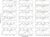 |
Fig. A.1 Individual gaussian fit for iron and nickel lines. In the case of blended features, deblending is performed by fitting a sum of two Gaussian components. |
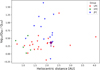 |
Fig. A.2 Comparison between 3I NH abundance with Cochran et al. (2012) database. |
All Tables
Detected Fe and Ni lines used for Gaussian fits to compute the number of atoms in the coma.
All Figures
|
Fig. 1 Frame of 3I/ATLAS at 600s taken in the sloan r filter from the same observing session of spectroscopy with the 0.67/0.92 m Schmidt telescope (INAF-OAPD), Asiago. The orientation of the long-slit is shown. |
| In the text | |
|
Fig. 2 Two-dimensional co-added spectrum of 3I/ATLAS with the sky and dust continuum removed. |
| In the text | |
|
Fig. 3 One-dimensional co-added frame of 3I/ATLAS. The blue and orange delta functions indicate the nickel and iron transitions for which the g factors were computed. |
| In the text | |
|
Fig. 4 Spatial distribution of iron, nickel, and the CN band. The solid line is the resulting MCMC best fit. The dashed lines are the best fit for the ρa profile. For comparison, the dust profile is also shown. The dust continuum used was 440–450 nm. |
| In the text | |
|
Fig. 5 Comparison between the computed iron and nickel parent scale lengths (with 3σ error bars) and the photoionisation values from Huebner & Mukherjee (2015). Different outflow velocities are shown: the highlighted region corresponds to the range of parent scale lengths obtained using the HCN outflow velocity from Biver et al. (2026); the segmented lines indicate the HCN scale lengths derived from ALMA observations (Roth et al. 2026); and the solid lines represent the scale lengths computed using the standard |
| In the text | |
|
Fig. 6 Reproduction of the plot of correlation between Q(Ni)/Q(Fe) and Q(NH)/Q(CN) from Hutsemékers et al. (2021) but including the results computed here. |
| In the text | |
|
Fig. A.1 Individual gaussian fit for iron and nickel lines. In the case of blended features, deblending is performed by fitting a sum of two Gaussian components. |
| In the text | |
|
Fig. A.2 Comparison between 3I NH abundance with Cochran et al. (2012) database. |
| In the text | |
Current usage metrics show cumulative count of Article Views (full-text article views including HTML views, PDF and ePub downloads, according to the available data) and Abstracts Views on Vision4Press platform.
Data correspond to usage on the plateform after 2015. The current usage metrics is available 48-96 hours after online publication and is updated daily on week days.
Initial download of the metrics may take a while.