


| Issue |
A&A
Volume 711, July 2026
|
|
|---|---|---|
| Article Number | A279 | |
| Number of page(s) | 9 | |
| Section | The Sun and the Heliosphere | |
| DOI | https://doi.org/10.1051/0004-6361/202659875 | |
| Published online | 21 July 2026 | |
Fine-scale downflows above flare ribbons captured by Solar Orbiter/EUI
1
School of Earth and Space Sciences, Peking University,
Beijing
100871,
PR
China
2
State Key Laboratory of Solar Activity and Space Weather, National Space Science Center, Chinese Academy of Sciences,
Beijing
100190,
PR
China
3
Leibniz Institute for Astrophysics Potsdam,
An der Sternwarte 16,
Potsdam
14482,
Germany
4
Plasma Dynamics Group, School of Electrical and Electronic Engineering, University of Sheffield,
Sheffield,
S1 3JD,
UK
5
Institute of Physics and Astronomy, University of Potsdam,
Karl-Liebknecht-Str. 24/25,
14476
Potsdam-Golm,
Germany
6
State Key Laboratory of Solar Activity and Space Weather, National Astronomical Observatories, Chinese Academy of Sciences,
Beijing
100101,
PR
China
7
Centre for Mathematical Plasma Astrophysics, KU Leuven,
Celestijnenlaan 200B,
3001
Leuven,
Belgium
★ Corresponding author: This email address is being protected from spambots. You need JavaScript enabled to view it.
Received:
15
March
2026
Accepted:
16
June
2026
Abstract
In solar flares, flare ribbons map chromospheric footpoints where flare energy deposition occurs. These locations are associated with field-aligned energy transport from the corona that results from energy liberated during magnetic reconnection. Recent chromospheric observations in the Hα and Hβ bands have revealed fine-scale downflow structures above flare ribbons, referred to as riblets. In this study, we identify similar downflow structures in the extreme-ultraviolet (EUV) wavelength using high-resolution observations from Solar Orbiter/EUI. These fine-scale downflows appear as downward-propagating, bright, and thread-like structures. They exhibit typical velocities of ~100 km s−1, lifetimes of ~15 s, and lengths of ~1.6 Mm. Based on their morphological and dynamical properties, we interpret these observed downflows as the EUV counterparts of the riblets that have previously been reported from chromospheric observations. This study presents EUV imaging of ~106 K downflows above flare ribbons. We interpret these downflows as a result of (1) the energisation and subsequent compression of pre-existing chromospheric fibrils due to particle beams or (2) adiabatic or shock-driven compression induced by the downward-propagating plasma from the corona. These fine-scale EUV riblets provide a new diagnostic tool for probing the dynamics of magnetic reconnection as well as energy transport and deposition during solar flares.
Key words: Sun: activity / Sun: atmosphere / Sun: corona / Sun: flares
© The Authors 2026
 Open Access article, published by EDP Sciences, under the terms of the Creative Commons Attribution License (https://creativecommons.org/licenses/by/4.0), which permits unrestricted use, distribution, and reproduction in any medium, provided the original work is properly cited.
This article is published in open access under the Subscribe to Open model. This email address is being protected from spambots. You need JavaScript enabled to view it. to support open access publication.
1 Introduction
Solar flares are magnetically driven, impulsive events that can release up to 1032 erg and radiate from radio to gamma rays (Fletcher et al. 2011; Benz 2017; Li et al. 2025). Despite extensive observations, the details of energy conversion from magnetic free energy to heating, particle acceleration, and mass motions are not yet fully understood. In the 2D CSHKP framework, the rising of a flux rope forms a current sheet beneath itself; reconnection proceeds within that sheet, and the released energy travels along field lines to the lower atmosphere where it is deposited (Carmichael 1964; Sturrock 1966; Hirayama 1974; Kopp & Pneuman 1976). Modern 3D studies extend this picture by emphasizing the roles of flux rope topology, quasi-separatrix layers (QSLs), and slipping reconnection in the energy release processes (Demoulin et al. 1996; Titov & Démoulin 1999; Isenberg & Forbes 2007; Aulanier et al. 2012; Li & Zhang 2014, 2015; Sun et al. 2023; Xing et al. 2024; Li et al. 2024; Xing et al. 2025; Tan et al. 2025b).
The principal agents for field-aligned energy transport in flares are still hotly debated. Beams of energetic particles (Holman et al. 2011; Krucker et al. 2011; Battaglia et al. 2015; Druett et al. 2017) and thermal conduction (Zarro & Lemen 1988; Brosius 2012; Ashfield & Longcope 2021; Kerr et al. 2026) are the most widely studied mechanisms, with some studies also investigating the potential of Alfvénic waves to deliver a non-negligible fraction of the energy (Fletcher & Hudson 2008; Russell & Fletcher 2013; Reep & Russell 2016). Transport of energy from the reconnection site via a combination of beams of energetic particles and thermal conduction has been proposed to deposit energy in the lower atmosphere when encountering higher-density structures. This energy deposition ionises, excites, and heats the local plasma, and also transfers momentum to the plasma within the flux tube. The beam-particle model has been supported by observations of strong hard X-ray (HXR) bremsstrahlung footpoints observed in flares (Hoyng et al. 1981; Fletcher & Hudson 2002). The brightening of the lower atmospheric emission at these sites leads to the appearance of elongated structures called flare ribbons.
Ribbons form in the chromosphere on opposite sides of the polarity inversion line (PIL), and subsequently elongate and separate (Fletcher & Hudson 2002; Fletcher et al. 2011). Many observations and 3D eruption models show that ribbons frequently exhibit a double-J morphology (Demoulin et al. 1996; Titov & Démoulin 1999; Titov 2007; Masson et al. 2009; Aulanier et al. 2012; Zhao et al. 2016; Janvier 2017; Sun et al. 2025). Observations of emission from ribbons have been interpreted in terms of energy deposition via thermal conduction and beams of particles in 1D models (Brown 1973; Emslie 1978; Somov et al. 1981; Ricchiazzi & Canfield 1983; Fisher et al. 1985; Canfield & Gayley 1987; Druett et al. 2017; Allred et al. 2020) and multi-dimensional models (Ruan et al. 2020; Druett et al. 2023, 2024). One critical feature that tests, and also predicts, behaviours via the modelled energy deposition methods is the generation of bi-directional field-aligned flows known as chromospheric evaporation (upflows) and condensation (downflows). Importantly, the characteristic plasma temperatures of observations that show upflows and downflows during ribbon formation and evolutions have supported a general picture of chromospheric and cool transition region lines (log (T/K) ≈ 4.0–5.0) with downflows (Milligan & Dennis 2009; Druett et al. 2017; Kerr 2022; Li et al. 2022; Polito et al. 2023), and hotter coronal lines (log (T/K) ≈ 6.3–7.2) with upflows (Zarro & Lemen 1988; Milligan & Dennis 2009; Tian et al. 2014, 2015; Li et al. 2019b, 2022, 2023). Lines in the log (T/K) ≈ 6.0 range have typically been reported to show redshifts, e.g. OVI–FeXIII lines (Milligan & Dennis 2009), but little imaging evidence exists to corroborate this.
Recently, high-resolution observations have offered the capability to resolve the fine-scale structure of flare ribbons. Previous studies have reported compact, rapidly evolving kernels or blobs that drift along flare ribbons (e.g. Young et al. 2013; Sharykin & Kosovichev 2014; Lörinčík et al. 2022; Thoen Faber et al. 2025; Zhang et al. 2025; French et al. 2025). In addition, Pietrow et al. (2024b) used the Swedish 1-m Solar Telescope (SST; Scharmer et al. 2003) to examine the spectral characteristics of substructures within flare ribbons. The effect of these substructures on the average flare spectrum was later followed up in both observations (Pietrow et al. 2024a; De Wilde et al. 2025) and simulations (Yu et al. 2025). Several studies have identified fine-scale upflow or downflow features located above flare ribbons through imaging observations. Using observations from the Interface Region Imaging Spectrograph (IRIS, De Pontieu et al. 2014) and the Atmospheric Imaging Assembly (AIA, Lemen et al. 2012) on board the Solar Dynamics Observatory (SDO, Pesnell et al. 2012), Li et al. (2019a) detected jet-like upflows with average velocities of approximately 70 km s−1, interpreted as signatures of chromospheric evaporation. Singh et al. (2025) analysed high-resolution Hα observations from the SST and reported ubiquitous ribbon-localized downflows during an X1.5 flare, with speeds of several tens of km s−1. They termed these features ‘riblets’ and suggested that they correspond to the redshifted structures observed at the leading edge of flare ribbons (Druett et al. 2017; Pietrow et al. 2024b). Thoen Faber et al. (2026) further conducted a statistical study of riblets using SST observations and identified redshifted emission components with line-of-sight velocities of 16–21 km s−1 and vertical extents of 620–1220 km in Hβ. While Chitta et al. (2026) recently presented high-cadence, high-resolution imaging from Solar Orbiter showing similar fine-scale downflowing structures in the EUV regime, a detailed quantitative analysis of these features remains absent. In this paper, we analyse the same eruptive event as Chitta et al. (2026) to further investigate these EUV downflows. By utilizing data from Solar Orbiter, we aim to fill the imaging gap in the existing literature regarding ribbon formation dynamics at the ~106 K level. Furthermore, we inspect the physical connectivity between ribbon substructures at chromospheric temperatures (log(T/K) ≈ 4.0) and those at coronal temperatures (log(T/K) ≥ 6.0).
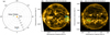 |
Fig. 1 Overview of the positions (a) and viewing geometry from Solar Orbiter (b), and SDO (c). The cyan square denotes the field of view (FoV) of HRIEUV. Since the HRIEUV FoV partially lies outside the solar disk, we define a smaller on-disk region (green square) within the FoV and re-project this region onto the SDO perspective. |
2 Observations
On 2024 September 30, an eruptive event occurred in NOAA AR 13842 near the west limb from the perspective of Solar Orbiter, and on the east limb as seen from Earth (see Fig. 1). This event was captured by the High Resolution Imager in the EUV (HRIEUV) telescope of the Extreme Ultraviolet Imager (EUI; Rochus et al. 2020) instrument on board the Solar Orbiter. During this time, the spacecraft was located 0.29 au from the Sun, corresponding to a spatial sampling of approximately 0.105 Mm per pixel, a factor of four above the typical AIA resolution of 0.43 Mm per pixel.
HRIEUV recorded a continuous sequence of images in 174 Å which is most sensitive to plasma around log(T/K) ≈ 6.0 (Berghmans et al. 2021; Chen et al. 2021). The data set covers nearly 1 hour of observations, from 22:55 to 23:55 UT, with a cadence of 2 s and an exposure time of 1.65 s. This exceptional combination of high spatial and temporal resolution enables a detailed inspection of the fine-scale structures of the flare ribbon. The flux rope began to rise around 23:20 UT and underwent a rapid eruption that continued until approximately 23:55 UT. During the main phase of this activity, an M7.6 flare developed within active region NOAA 13842. The mechanism of energy release associated with this event has been investigated by Chitta et al. (2026). During the eruption, the filament exhibited a clear untwisting motion and generated a number of smallscale coronal jets, which have been analysed in recent studies (Gao et al. 2025; Bura et al. 2025; Tan et al. 2025a; Wallace & Antolin 2025). We also employed full-disk 174 Å imaging from the EUI/Full Sun Imager (FSI) on board Solar Orbiter to provide a global context of the event. A comparison between the full-disk observations from Solar Orbiter and SDO is shown in Figures 1c and 1d. To investigate the flare evolution, we also used soft X-ray (SXR) flux observations from the GOES/XRS instrument and HXR observations from the Spectrometer/Telescope for Imaging X-rays (STIX; Krucker et al. 2020) on board Solar Orbiter. The GOES/XRS data provide the temporal evolution of the flare emission, while STIX observations are used to identify the timing of the impulsive energy release.
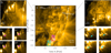 |
Fig. 2 Overview of the downflows in this event. Panel (a) shows the field of view of the HRIEUV observation. The boxes labelled R1 and R2 mark two different flare-ribbon regions. Panels (b) and (c) present zoomed-in views of regions R1 and R2. Panels (b1–b4) and (c1–c4) display the detailed temporal evolution of two selected individual downflows. The fields of view of these panels are indicated by the black squares in panels (b) and (c), respectively. The blue arrows indicate the trajectories of the downflows. The pink and cyan arrows mark the locations of the downflows in the corresponding frame. (An online animation is available for this figure.) |
3 Results
As the filament rises, the flare ribbons appear and develop into several segments of flare ribbons. Fine-scale recurrent downflows above the flare ribbons become discernible starting from approximately 23:38 UT, as also reported by Chitta et al. (2026). Figure 2 provides an overview of these downflows. We focus our analysis on two specific areas, Region 1 (R1) and Region 2 (R2), as indicated in the figure. Panels b1–b4 and c1–c4 show zoomed-in views of the evolution of two individual downflows in Region 1 and Region 2. These downflows appear as thread-like, slender structures that are bright in 174 Å and move toward the flare ribbon. Their morphology and occurrence above the ribbons closely resemble the riblet structures reported by Singh et al. (2025) and Thoen Faber et al. (2026). Figure 3 further shows the corresponding locations of the downflows in SDO/AIA 171 Å and 1600 Å. The ribbons corresponding to regions R1 and R2 are indicated by the pink and cyan arrows, respectively. The 1600 Å images show that the downflows occur in two spatially separated ribbon regions, denoted as R1 and R2. Moreover, it should be noted that the downflows in this event are difficult to resolve with the spatial resolution of AIA. However, some faint brightenings may be present in the unsaturated portions of the flare ribbon, although the available AIA observations do not allow a reliable identification of their nature.
Figures 4a–d show the temporal evolution of Region 2. The downflow locations are not stationary, but instead exhibit a gradual displacement over time. This behaviour may correspond to successive reconnection between the erupting flux rope and progressively higher overlying magnetic field lines. In panel e, we plot the temporal evolution of the SXR and HXR emission of the flare. From the figure, we can see that the downflows observed by Solar Orbiter occur during the impulsive phase of the flare.
We note that the riblet-like features in the HRIEUV images evolve rapidly, making it inaccurate to extract the physical parameters of the downflows by placing fixed slices along their trajectories. To account for this rapid evolution, we instead analysed each downflow manually on a frame-by-frame basis using the open-source software Tracker1. This approach allows us to determine the lifetime, characteristic width, and projected velocity of individual downflowing features more accurately. An example of the tracking procedure and parameter measurements is presented in Appendix A. In total, we identified 43 unambiguous downflows in Region 1 and 48 in Region 2. The statistical distributions of their properties are shown in Fig. 5. Since the results from the two regions are basically consistent, we infer that the downflows likely share the same physical origin. Compared with Singh et al. (2025), who adopted a similar measurement strategy, the average lifetimes of the downflows in our event are 14.7 and 16.7 s for Regions 1 and 2, respectively – close to their reported value of ~12 s. Such short timescales indicate that these features are difficult to detect with SDO/AIA, which has a cadence of 12 s. The lengths of the downflows are 1.5 and 1.7 Mm, slightly larger than the ~0.95 Mm reported by Singh et al. (2025), and 0.62–1.2 Mm measured by Thoen Faber et al. (2026). The averaged velocities, 91 and 100 km s−1 for the two regions, exceed the ~47 km s−1 reported in Singh et al. (2025). The starting times of the downflows are distributed almost uniformly throughout the entire eruption.
Overall, the observed lifetimes, lengths, and velocities resemble the properties of the riblets identified in chromospheric lines by Singh et al. (2025) and Thoen Faber et al. (2026). We therefore interpret the fine-scale downflows reported here as the EUV counterparts of riblets.
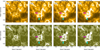 |
Fig. 3 Overview of the same active region as in Fig. 2, observed with SDO/AIA 171 Å and 1600 Å at four different times. The pink and cyan arrows mark the same locations as in Fig. 2. |
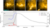 |
Fig. 4 Temporal evolution of Region 2 observed by EUI and the SXR and HXR emission of the flare. Panels (a)–(d) show the evolution of Region 2, while panel (e) displays the GOES 1–8 Å SXR light curve together with the STIX 4–10 keV and 25–50 keV HXR light curves. Details of the HXR data processing are described in Tan et al. (2025a). The grey shaded region indicates the EUI observing time span. The vertical dashed lines mark the times corresponding to panels (a)–(d). |
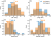 |
Fig. 5 Histograms of the statistical properties of the downflows identified in Region 1 and Region 2. The values marked in each panel indicate the corresponding mean values. The starting time in panel (d) corresponds to the first appearance of the downflow. |
4 Discussion
In this section, we discuss our observations and outline several possible physical origins of these manifestations, together with suggestions for future observations that could help discriminate between these scenarios.
4.1 EUV ribbon substructures and the association with chromospheric riblets
This set of observations extends the observational coverage of flare-related downflows from previously reported condensation at temperatures of ~105 K to evaporation at coronal temperatures of ~1 × 10⁶ K for flare ribbon formation such as Milligan & Dennis (2009), Polito et al. (2023), and Pietrow et al. (2024b). We observe widespread downflowing plasma in the ~1 × 10⁶ K range at the footpoints of flare loops. This information is critical to test, validate and discriminate among energy transport, deposition, and atmospheric response theories via simulations.
Additionally, thanks to recent sub-second chromospheric imaging of riblets we are able to compare the dynamics of ~1 × 10⁶ K plasma with that of ~1 × 10⁴ K plasma (Singh et al. 2025; Thoen Faber et al. 2026). The structures we report have sufficiently similar morphology, lifetimes, and locations to infer that these features are likely EUV riblets, that are higher, hotter extensions of chromospheric riblet fine structures. It should also be noted that the 174 Å passband has a broad temperature response extending well beyond its peak sensitivity near ~1 MK. Therefore, the structures identified here may correspond to the same physical features previously observed in cooler chromospheric lines, viewed through a different temperature response regime. Differences in reported lengths and velocity may arise from (1) the gradients in the evolving plasma, where the physically higher, longer, and hotter components have greater velocities than the lower, cooler, regions which have stronger pressure gradients or (2) from different projection geometries between these events. Again, this issue could be more conclusively addressed through coordinated multi-wavelength observations covering a broader temperature range, combining Solar Orbiter with chromosphere-targeting telescopes and future spectroscopic diagnostics (e.g. MUSE, EUVST).
4.2 Physical interpretation of the riblets
Such connected fine structures imply that flare energy deposition drives coherent plasma structures propagating downwards during ribbon formation that contains multi-thermal plasma with temperatures between ~1 × 10⁴ K and ~1 × 10⁶ K. Previous chromospheric riblet studies have attempted to explain the physical origin of riblets: Singh et al. (2025) suggested that the riblets correspond to redshifted destruction of chromospheric structures at the expanding edges of flare ribbons (Druett et al. 2017; Pietrow et al. 2024b), whereas Thoen Faber et al. (2026) proposed that riblets are associated with tearing-mode instabilities in the reconnection current sheet (Dahlin et al. 2025) to account for the recurrent nature of the downflows. However, these interpretations primarily focus on the association with magnetic reconnection but do not explicitly address the mechanisms by which flare energy is transported to the lower atmosphere to produce the observed downflows. In the following, we propose two scenarios to explain these observations.
4.2.1 Possible Scenario 1: energisation and compression of fibrils
If flare ribbon formation compresses former active region chromospheric structures to lower geometric heights, then the main candidates showing correspondence with riblets are the fibrils (or spicules when seen from the side). Chromospheric fibrils extend upward from the chromosphere toward the low corona. Dynamic fibrils in active regions have typical lengths of ~1250 km, but can vary with local conditions, ranging from 400 to 5200 km when observed in Hα (De Pontieu et al. 2007; Samanta et al. 2019; Joshi et al. 2026; Chen 2026) or analysed in magnetohydrodynamic simulations (Hansteen et al. 2006; Chandra et al. 2025). Under normal conditions they are theorised to be launched due to the actions of p-modes or magnetic reconnection, and have parabolic paths in height-time diagrams with maximum ascent or descent velocities achieved near launch or termination, of 15–20 km s−1 but reaching to 35 km s−1 in some cases. Fibrils are ubiquitously distributed throughout active regions (see Fig. 7 of Pietrow et al. 2024b). The lengths of these structures are consistent with the observed features. However, the observed higher velocities and non-parabolic height-time trajectories suggest that these flows are driven by additional energy deposition and plasma compression from the flare, rather than the simple ballistic collapse of existing structures. Additionally this picture is corroborated by the lower subsequent formation heights of flare ribbon emission (Martínez Oliveros et al. 2012; Krucker et al. 2015; Li et al. 2016; Kuridze et al. 2020; Pietrow et al. 2024b) as well as geometric observational arguments from overlapping structures in flare observations (Pietrow et al. 2024b).
When newly reconnected flare field lines in the current sheet retract and relax, they form coronal loops anchored at their chromospheric footpoints, which correspond to the leading edges of the flare ribbons. This magnetic restructuring significantly alters the surrounding environment of the pre-existing fibrils. Energy is deposited via field-aligned thermal conduction or non-local transport by energetic particle beams from the reconnection site, leading to the ionization, excitation, and heating of the flux-tube plasma, as well as the transfer of momentum. Under the thermal conduction scenario, the observed downward motion may not represent a bulk physical plasma flow, but rather the propagation of a heating front (De Pontieu et al. 2017). In this framework, the downflow is an apparent motion where the transition region is pushed toward lower, denser atmospheric layers. For this interpretation to be viable, the measured downward velocities of the bright features must be consistent with the propagation speed of a conduction front as it heats the plasma to EUV-emitting temperatures. On the other hand, recent on-disk Doppler shift observations by Pietrow et al. (2024b) and side-view observations by Singh et al. (2025); Thoen Faber et al. (2026) show mutually consistent downflow velocities, suggesting that these features are likely associated with real plasma motions. Given the strong morphological similarities between those chromospheric riblets and the structures reported here, our observations may also favour a physical downflow interpretation. Nevertheless, we cannot fully exclude that some of the observed motions are related to the propagation of heating fronts. A schematic illustration of the beam-driven scenario is presented in Figure 6a.
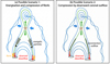 |
Fig. 6 Cartoon scenarios of the observed downflows. The five-pointed star symbol indicates the magnetic reconnection site. This sketch is adapted from Lysenko et al. (2020). |
4.2.2 Possible Scenario 2: compression by downward coronal outflow
When magnetic reconnection occurs high in the corona, reconnection outflows are generated (Kopp & Pneuman 1976; Priest & Forbes 2000). These outflows may then propagate downward along the newly formed post flare loops into the denser lower atmosphere (e.g. Tian et al. 2014). During this process, they can undergo adiabatic compression, which increases the plasma density and temperature and may lead to the formation of bright downflowing structures within the flux tube. Another related possibility is that the enhanced density in the low atmosphere reduces the local Alfvén speed relative to that in the corona (Hollweg 1981; van Ballegooijen et al. 2011). In this case, the downward outflows may exceed the local Alfvén speed near the chromosphere and form a termination shock (Shibata & Tanuma 2001; Aurass et al. 2002; Mann et al. 2009; Cai et al. 2019). Such a shock would compress the ambient plasma and increase its temperature and density (Forbes & Priest 1983; Takasao et al. 2015), allowing the downflows to appear as bright EUV structures in low altitudes. In addition, similar to Scenario 1, the observed downward motion may not necessarily correspond entirely to bulk plasma flows. Part of the apparent motion could also be associated with the propagation of a heating or compression front along the magnetic structure, which may contribute to the observed EUV brightening. The cartoon illustration of this scenario is shown in Figure 6b.
An alternative possible origin of the observed downflows is coronal rain, which also consists of downflowing plasma along post-flare loops, typically occurring during the decay phase of flares (Scullion et al. 2016; Ruan et al. 2021; Şahin & Antolin 2024). To examine this possibility, we compare the occurrence times of the downflows with the GOES soft X-ray and STIX hard X-ray light curves (Figure 4). We find that the downflows appear almost simultaneously with the flare onset, and a large number of downflows are already present during the impulsive phase. This temporal behaviour is inconsistent with the typical evolution of coronal rain, which is generally associated with cooling processes during the later decay phase (e.g. Martínez Oliveros et al. 2014; Chen et al. 2022; Qiao et al. 2024). Therefore, we consider it unlikely that coronal rain is the dominant mechanism responsible for the downflows analysed in this work.
The coronal-outflow-driven compression scenario is also supported by large-scale downflow observations (Sun et al. 2024; Wu et al. 2025). Sun et al. (2024) observed large-scale downflows near the footpoints of a polar crown filament. The downflows can be observed across all SDO/AIA passbands with speeds of 92–144 km s−1, and similar phenomena were later found in several filament eruptions (Wu et al. 2025). These downflows share several key features with the riblet-like structures reported here: they occur along flare ribbons, manifest as EUV bright structures, appear only at relatively low altitudes, exhibit thread-like EUV morphology, and show recurrent behaviour. In those events, the heights of the downflows are far beyond the scale of chromospheric fibrils and therefore cannot be explained by Scenario 1. Instead, they were interpreted as a consequence of the conversion of kinetic energy from falling filament material into thermal energy, supported by the clear observational evidence that the downflows originate directly from the descending filament material (see Fig. 2g in Sun et al. 2024). By analogy, a similar physical mechanism may operate in our event. However, instead of a massive amount of filament material falling back to the lower atmosphere, the falling structures here would represent downward reconnection outflows. Because reconnection outflows are far less massive than filament plasma, the resulting downflows would naturally be smaller in scale and less pronounced than those associated with filament eruptions.
Additional hints supporting this scenario might also be found in flare numerical simulations (e.g. Ruan et al. 2023; Ye et al. 2023; Druett et al. 2024). These models show that reconnection outflows impact the top of the flare arcade and subsequently propagate downward along the arcade. However, whether such downward-propagating flows can further compress plasma at lower heights and manifest as the downflows observed here remains unclear, and will require future numerical simulations to be investigated in detail.
4.3 Connection to three-dimensional eruption models
In Figs. 4a–d, we observe continuous drifts in the locations of the downflows. This behaviour may correspond to successive reconnection between the erupting flux rope and progressively higher overlying magnetic field lines, causing the corresponding magnetic footpoints to move farther away from the eruption centre. This suggests that such downflows could serve as observational tracers of the evolution of magnetic reconnection during eruptive flares and may help us better understand the different reconnection processes involved in flux rope eruptions.
Additionally, the recurrent nature of the observed downflows may be explained by tearing-mode instabilities developing in the reconnection current sheet, as also suggested by Thoen Faber et al. (2026). Dahlin et al. (2025) performed three-dimensional magnetohydrodynamic eruption simulations and found that tearing-mode instabilities arise naturally in turbulent current sheets. The resulting intermittent reconnection can produce recurrent fine structures in flare ribbons. However, their analysis focused primarily on horizontal ribbon substructures, rather than on vertical motions such as the downflows reported here. Nevertheless, if reconnection energy release is intermittent, it is expected to generate intermittent particle beams and downward reconnection outflows (plasmoids) as well. These intermittent energy and momentum injections could then lead to the recurrent downflows observed in this work. If this interpretation is correct, the waiting times and occurrence frequencies of the downflows may provide valuable observational constraints on tearing-mode-driven magnetic reconnection.
5 Conclusion
In this work, we use Solar Orbiter/EUI observations to report fine-scale downflow structures above flare ribbons in EUV 174 Å. These features appear as downward-moving, bright, thread-like structures with speeds of ~100 km s−1, lifetimes of ~15 s, and lengths of ~1.6 Mm. We interpret these structures as EUV riblets, the coronal ~106 K fine structure extensions of the chromospheric ~104 K ribbon fine-structures observed in chromospheric lines (Singh et al. 2025; Thoen Faber et al. 2026). Their spatial and temporal scales are extremely small, making such fine structures difficult to be resolved with SDO/AIA. In contrast, the high-resolution EUV observations from Solar Orbiter/EUI allow us to identify these downflows clearly.
We discuss two possible scenarios for the formation of these structures: Flare-related energy release, in the form of energetic particle beams (Scenario 1) or downward plasma drains (Scenario 2), can lead to energy deposition at relatively low atmospheric heights, manifesting observationally as the downflows reported here. The observed downward motions may correspond to real plasma flows or to the propagation of heating fronts, and the current observations do not allow us to directly distinguish between these possibilities. Because both scenarios are intrinsically linked to magnetic reconnection, these downflows are expected to occur at reconnection footpoints, that is, along flare ribbons. The recurrent nature of the downflows may further be explained by tearing-mode instabilities operating in the reconnection current sheet.
We suggest that such fine-scale downflows may be a ubiquitous phenomenon accompanying solar flares. Confirming this possibility will require additional high-resolution observations, particularly those capable of resolving the relevant spatial and temporal scales. Systematic campaigns with Solar Orbiter/EUI and co-observations with high-resolution ground-based telescopes capable of observing the chromosphere will be essential to determine how commonly these structures occur and how they relate to the energy release and plasma dynamics in flares. Moreover, ~106 K downflows provide an observational constraint that simulations should test, namely whether plasma in this temperature response channel can produce downflowing substructures when energy is transported primarily via the proposed mechanisms. This helps improve our understanding of energy transport processes during solar flares.
Data availability
Movie associated to Fig. 2 is available at https://www.aanda.org.
Acknowledgements
This work is supported by the Strategic Priority Research Program of the Chinese Academy of Sciences (grant no. XDB0560000), the National Natural Science Foundation of China(12425301, 425B2024), China’s Space Origins Exploration Program, and the Specialized Research Fund for State Key Laboratory of Solar Activity and Space Weather. A.P. is supported by grant PI 2102/1-1 from the Deutsche Forschungsgemeinschaft (DFG). H.T. is also supported by the New Cornerstone Science Foundation through the Xplorer Prize. S.T. was supported by the German Space Agency (DLR), grant number 50 OT 2304.
References
- Allred, J. C., Alaoui, M., Kowalski, A. F., & Kerr, G. S. 2020, ApJ, 902, 16 [NASA ADS] [CrossRef] [Google Scholar]
- Ashfield, W. H., & Longcope, D. W. 2021, ApJ, 912, 25 [Google Scholar]
- Aulanier, G., Janvier, M., & Schmieder, B. 2012, A&A, 543, A110 [NASA ADS] [CrossRef] [EDP Sciences] [Google Scholar]
- Aurass, H., Vršnak, B., & Mann, G. 2002, A&A, 384, 273 [NASA ADS] [CrossRef] [EDP Sciences] [Google Scholar]
- Battaglia, M., Kleint, L., Krucker, S., & Graham, D. 2015, ApJ, 813, 113 [Google Scholar]
- Benz, A. O. 2017, Liv. Rev. Sol. Phys., 14, 2 [Google Scholar]
- Berghmans, D., Auchère, F., Long, D. M., et al. 2021, A&A, 656, L4 [NASA ADS] [CrossRef] [EDP Sciences] [Google Scholar]
- Brosius, J. W. 2012, ApJ, 754, 54 [Google Scholar]
- Brown, J. C. 1973, Sol. Phys., 28, 151 [NASA ADS] [CrossRef] [Google Scholar]
- Bura, A., Shrivastav, A. K., Patel, R., et al. 2025, ApJ, 988, L65 [Google Scholar]
- Cai, Q., Shen, C., Raymond, J. C., et al. 2019, MNRAS, 489, 3183 [Google Scholar]
- Canfield, R. C., & Gayley, K. G. 1987, ApJ, 322, 999 [NASA ADS] [CrossRef] [Google Scholar]
- Carmichael, H. 1964, in NASA Special Publication, 50, ed. W. N. Hess, 451 [Google Scholar]
- Chandra, S., Cameron, R., Przybylski, D., et al. 2025, A&A, 701, A294 [NASA ADS] [CrossRef] [EDP Sciences] [Google Scholar]
- Chen, C. 2026, Earth Planet. Phys., 10, 438 [Google Scholar]
- Chen, Y., Przybylski, D., Peter, H., et al. 2021, A&A, 656, L7 [NASA ADS] [CrossRef] [EDP Sciences] [Google Scholar]
- Chen, H., Tian, H., Li, L., et al. 2022, A&A, 659, A107 [NASA ADS] [CrossRef] [EDP Sciences] [Google Scholar]
- Chitta, L. P., Pontin, D. I., Priest, E. R., et al. 2026, A&A, 705, A113 [NASA ADS] [CrossRef] [EDP Sciences] [Google Scholar]
- Dahlin, J. T., Antiochos, S. K., Wyper, P. F., Qiu, J., & DeVore, C. R. 2025, ApJ, 993, 31 [Google Scholar]
- De Pontieu, B., Hansteen, V. H., Rouppe van der Voort, L., van Noort, M., & Carlsson, M. 2007, ApJ, 655, 624 [Google Scholar]
- De Pontieu, B., Title, A. M., Lemen, J. R., et al. 2014, Sol. Phys., 289, 2733 [Google Scholar]
- De Pontieu, B., De Moortel, I., Martinez-Sykora, J., & McIntosh, S. W. 2017, ApJ, 845, L18 [NASA ADS] [CrossRef] [Google Scholar]
- De Wilde, M., Pietrow, A. G. M., Druett, M. K., et al. 2025, A&A, 700, A275 [NASA ADS] [CrossRef] [EDP Sciences] [Google Scholar]
- Demoulin, P., Henoux, J. C., Priest, E. R., & Mandrini, C. H. 1996, A&A, 308, 643 [NASA ADS] [Google Scholar]
- Druett, M., Scullion, E., Zharkova, V., et al. 2017, Nat. Commun., 8, 15905 [NASA ADS] [CrossRef] [Google Scholar]
- Druett, M. K., Ruan, W., & Keppens, R. 2023, Sol. Phys., 298, 134 [NASA ADS] [CrossRef] [Google Scholar]
- Druett, M., Ruan, W., & Keppens, R. 2024, A&A, 684, A171 [NASA ADS] [CrossRef] [EDP Sciences] [Google Scholar]
- Emslie, A. G. 1978, ApJ, 224, 241 [NASA ADS] [CrossRef] [Google Scholar]
- Fisher, G. H., Canfield, R. C., & McClymont, A. N. 1985, ApJ, 289, 414 [NASA ADS] [CrossRef] [Google Scholar]
- Fletcher, L., & Hudson, H. S. 2002, Sol. Phys., 210, 307 [Google Scholar]
- Fletcher, L., & Hudson, H. S. 2008, ApJ, 675, 1645 [Google Scholar]
- Fletcher, L., Dennis, B. R., Hudson, H. S., et al. 2011, Space Sci. Rev., 159, 19 [Google Scholar]
- Forbes, T. G., & Priest, E. R. 1983, Sol. Phys., 84, 169 [Google Scholar]
- French, R. J., Kazachenko, M. D., Berghmans, D., et al. 2025, ApJ, 995, L54 [Google Scholar]
- Gao, Y., Tian, H., Berghmans, D., et al. 2025, ApJ, 985, L12 [Google Scholar]
- Hansteen, V. H., De Pontieu, B., Rouppe van der Voort, L., van Noort, M., & Carlsson, M. 2006, ApJ, 647, L73 [Google Scholar]
- Hirayama, T. 1974, Sol. Phys., 34, 323 [Google Scholar]
- Hollweg, J. V. 1981, Sol. Phys., 70, 25 [Google Scholar]
- Holman, G. D., Aschwanden, M. J., Aurass, H., et al. 2011, Space Sci. Rev., 159, 107 [NASA ADS] [CrossRef] [Google Scholar]
- Hoyng, P., Duijveman, A., Boelee, A., et al. 1981, ApJ, 244, L153 [Google Scholar]
- Isenberg, P. A., & Forbes, T. G. 2007, ApJ, 670, 1453 [NASA ADS] [CrossRef] [Google Scholar]
- Janvier, M. 2017, J. Plasma Phys., 83, 535830101 [NASA ADS] [CrossRef] [Google Scholar]
- Joshi, R., Rouppe van der Voort, L., Aulanier, G., et al. 2026, A&A, 706, A369 [NASA ADS] [CrossRef] [EDP Sciences] [Google Scholar]
- Kerr, G. S. 2022, Front. Astron. Space Sci., 9, 1060856 [NASA ADS] [CrossRef] [Google Scholar]
- Kerr, G. S., Krucker, S., Allred, J. C., et al. 2026, Nat. Astron., 10, 202 [Google Scholar]
- Kopp, R. A., & Pneuman, G. W. 1976, Sol. Phys., 50, 85 [Google Scholar]
- Krucker, S., Hudson, H. S., Jeffrey, N. L. S., et al. 2011, ApJ, 739, 96 [NASA ADS] [CrossRef] [Google Scholar]
- Krucker, S., Saint-Hilaire, P., Hudson, H. S., et al. 2015, ApJ, 802, 19 [CrossRef] [Google Scholar]
- Krucker, S., Hurford, G. J., Grimm, O., et al. 2020, A&A, 642, A15 [NASA ADS] [CrossRef] [EDP Sciences] [Google Scholar]
- Kuridze, D., Mathioudakis, M., Heinzel, P., et al. 2020, ApJ, 896, 120 [NASA ADS] [CrossRef] [Google Scholar]
- Lemen, J. R., Title, A. M., Akin, D. J., et al. 2012, Sol. Phys., 275, 17 [Google Scholar]
- Li, T., & Zhang, J. 2014, ApJ, 791, L13 [NASA ADS] [CrossRef] [Google Scholar]
- Li, T., & Zhang, J. 2015, ApJ, 804, L8 [NASA ADS] [CrossRef] [Google Scholar]
- Li, Y., Qiu, J., Longcope, D. W., Ding, M. D., & Yang, K. 2016, ApJ, 823, L13 [Google Scholar]
- Li, X., Zhang, J., Yang, S., & Hou, Y. 2019a, PASJ, 71, 14 [Google Scholar]
- Li, Y., Ding, M. D., Hong, J., Li, H., & Gan, W. Q. 2019b, ApJ, 879, 30 [NASA ADS] [CrossRef] [Google Scholar]
- Li, D., Hong, Z., & Ning, Z. 2022, ApJ, 926, 23 [NASA ADS] [CrossRef] [Google Scholar]
- Li, D., Li, C., Qiu, Y., et al. 2023, ApJ, 954, 7 [Google Scholar]
- Li, D., Hou, Z., Bai, X., et al. 2024, Sci. China E: Technol. Sci., 67, 1592 [Google Scholar]
- Li, Y., Huang, S., Xu, S., et al. 2025, Earth Planet. Phys., 9, 171 [Google Scholar]
- Lörinčík, J., Polito, V., De Pontieu, B., Yu, S., & Freij, N. 2022, Front. Astron. Space Sci., 9, 334 [Google Scholar]
- Lysenko, A. L., Frederiks, D. D., Fleishman, G. D., et al. 2020, Phys. Usp., 63, 818 [CrossRef] [Google Scholar]
- Mann, G., Warmuth, A., & Aurass, H. 2009, A&A, 494, 669 [NASA ADS] [CrossRef] [EDP Sciences] [Google Scholar]
- Martínez Oliveros, J.-C., Hudson, H. S., Hurford, G. J., et al. 2012, ApJ, 753, L26 [CrossRef] [Google Scholar]
- Martínez Oliveros, J.-C., Krucker, S., Hudson, H. S., et al. 2014, ApJ, 780, L28 [Google Scholar]
- Masson, S., Pariat, E., Aulanier, G., & Schrijver, C. J. 2009, ApJ, 700, 559 [Google Scholar]
- Milligan, R. O., & Dennis, B. R. 2009, ApJ, 699, 968 [NASA ADS] [CrossRef] [Google Scholar]
- Pesnell, W. D., Thompson, B. J., & Chamberlin, P. C. 2012, Sol. Phys., 275, 3 [Google Scholar]
- Pietrow, A. G. M., Cretignier, M., Druett, M. K., et al. 2024a, A&A, 682, A46 [NASA ADS] [CrossRef] [EDP Sciences] [Google Scholar]
- Pietrow, A. G. M., Druett, M. K., & Singh, V. 2024b, A&A, 685, A137 [NASA ADS] [CrossRef] [EDP Sciences] [Google Scholar]
- Polito, V., Kerr, G. S., Xu, Y., Sadykov, V. M., & Lorincik, J. 2023, ApJ, 944, 104 [NASA ADS] [CrossRef] [Google Scholar]
- Priest, E., & Forbes, T. 2000, Magnetic Reconnection: MHD Theory and Applications (Cambridge, UK: Cambridge University Press) [Google Scholar]
- Qiao, F., Li, L., Tian, H., et al. 2024, ApJ, 973, 57 [Google Scholar]
- Reep, J. W., & Russell, A. J. B. 2016, ApJ, 818, L20 [Google Scholar]
- Ricchiazzi, P. J., & Canfield, R. C. 1983, ApJ, 272, 739 [Google Scholar]
- Rochus, P., Auchère, F., Berghmans, D., et al. 2020, A&A, 642, A8 [NASA ADS] [CrossRef] [EDP Sciences] [Google Scholar]
- Ruan, W., Xia, C., & Keppens, R. 2020, ApJ, 896, 97 [NASA ADS] [CrossRef] [Google Scholar]
- Ruan, W., Zhou, Y., & Keppens, R. 2021, ApJ, 920, L15 [NASA ADS] [CrossRef] [Google Scholar]
- Ruan, W., Yan, L., & Keppens, R. 2023, ApJ, 947, 67 [NASA ADS] [CrossRef] [Google Scholar]
- Russell, A. J. B., & Fletcher, L. 2013, ApJ, 765, 81 [Google Scholar]
- Şahin, S., & Antolin, P. 2024, ApJ, 970, 106 [Google Scholar]
- Samanta, T., Tian, H., Yurchyshyn, V., et al. 2019, Science, 366, 890 [NASA ADS] [CrossRef] [Google Scholar]
- Scharmer, G. B., Bjelksjo, K., Korhonen, T. K., Lindberg, B., & Petterson, B. 2003, in Proc. SPIE, 4853, Innovative Telescopes and Instrumentation for Solar Astrophysics, eds. S. L. Keil, & S. V. Avakyan, 341 [Google Scholar]
- Scullion, E., Rouppe van der Voort, L., Antolin, P., et al. 2016, ApJ, 833, 184 [NASA ADS] [CrossRef] [Google Scholar]
- Sharykin, I. N., & Kosovichev, A. G. 2014, ApJ, 788, L18 [NASA ADS] [CrossRef] [Google Scholar]
- Shibata, K., & Tanuma, S. 2001, Earth Planets Space, 53, 473 [NASA ADS] [CrossRef] [Google Scholar]
- Singh, V., Scullion, E., Botha, G. J. J., et al. 2025, arXiv e-prints [arXiv:2507.01169] [Google Scholar]
- Somov, B. V., Syrovatskii, S. I., & Spektor, A. R. 1981, Sol. Phys., 73, 145 [Google Scholar]
- Sturrock, P. A. 1966, Nature, 211, 695 [Google Scholar]
- Sun, Z., Li, T., Tian, H., et al. 2023, ApJ, 953, 148 [CrossRef] [Google Scholar]
- Sun, Z., Tian, H., Li, T., Liu, R., & Duan, Y. 2024, ApJ, 974, 205 [NASA ADS] [CrossRef] [Google Scholar]
- Sun, Z., Li, T., Bian, X., et al. 2025, ApJ, 990, 45 [Google Scholar]
- Takasao, S., Matsumoto, T., Nakamura, N., & Shibata, K. 2015, ApJ, 805, 135 [NASA ADS] [CrossRef] [Google Scholar]
- Tan, G., Hou, Y., & Tian, H. 2022, MNRAS, 516, 3120 [Google Scholar]
- Tan, S., Warmuth, A., Schuller, F., et al. 2025a, A&A, 702, A189 [NASA ADS] [CrossRef] [EDP Sciences] [Google Scholar]
- Tan, S., Warmuth, A., Schuller, F., et al. 2025b, A&A, 702, A88 [NASA ADS] [CrossRef] [EDP Sciences] [Google Scholar]
- Thoen Faber, J., Joshi, R., Rouppe van der Voort, L., et al. 2025, A&A, 693, A8 [NASA ADS] [CrossRef] [EDP Sciences] [Google Scholar]
- Thoen Faber, J., Joshi, R., Rouppe van der Voort, L., et al. 2026, A&A, 705, A174 [NASA ADS] [CrossRef] [EDP Sciences] [Google Scholar]
- Tian, H., Li, G., Reeves, K. K., et al. 2014, ApJ, 797, L14 [Google Scholar]
- Tian, H., Young, P. R., Reeves, K. K., et al. 2015, ApJ, 811, 139 [NASA ADS] [CrossRef] [Google Scholar]
- Titov, V. S. 2007, ApJ, 660, 863 [Google Scholar]
- Titov, V. S., & Démoulin, P. 1999, A&A, 351, 707 [NASA ADS] [Google Scholar]
- van Ballegooijen, A. A., Asgari-Targhi, M., Cranmer, S. R., & DeLuca, E. E. 2011, ApJ, 736, 3 [Google Scholar]
- Wallace, T., & Antolin, P. 2025, MNRAS, 544, 1758 [Google Scholar]
- Wu, Y., Liu, R., Luo, R., & Wang, W. 2025, ApJ, 987, 115 [Google Scholar]
- Xing, C., Aulanier, G., Cheng, X., Xia, C., & Ding, M. 2024, ApJ, 966, 70 [Google Scholar]
- Xing, C., Cheng, X., Aulanier, G., & Ding, M. 2025, ApJ, 986, 37 [Google Scholar]
- Ye, J., Raymond, J. C., Mei, Z., et al. 2023, ApJ, 955, 88 [NASA ADS] [CrossRef] [Google Scholar]
- Young, P. R., Doschek, G. A., Warren, H. P., & Hara, H. 2013, ApJ, 766, 127 [NASA ADS] [CrossRef] [Google Scholar]
- Yu, H. C., Hong, J., & Ding, M. D. 2025, A&A, 694, A315 [NASA ADS] [CrossRef] [EDP Sciences] [Google Scholar]
- Zarro, D. M., & Lemen, J. R. 1988, ApJ, 329, 456 [NASA ADS] [CrossRef] [Google Scholar]
- Zhang, Y., Li, T., Hou, Y., et al. 2025, ApJ, 982, L9 [Google Scholar]
- Zhao, J., Gilchrist, S. A., Aulanier, G., et al. 2016, ApJ, 823, 62 [Google Scholar]
Appendix A An example of the parameter measurement
To determine the projected velocities and lifetimes of the downflows, we manually tracked the front of each feature on a frame-by-frame basis using the open-source software Tracker. The software serves as an interactive tool to facilitate the identification of feature trajectories, while the underlying method remains a manual tracking procedure similar to those adopted in previous studies (e.g. Tan et al. 2022; Singh et al. 2025; Tan et al. 2025a).
Since Tracker operates on video files, the original dataset was first converted into a video and then imported into the software. An x–y coordinate system and spatial scale were added. In the present analysis, the absolute choice of the coordinate origin and axis orientation is not important, since we only require the relative displacement of the tracked features. After these steps, the front of each downflow feature was manually identified and tracked throughout its evolution. Figure A.1 shows a representative example of the tracking procedure adopted in this work. Using the manually selected front positions in successive frames, we calculated the projected speed of the downflow. Since no clear acceleration or deceleration was found in most cases, we simply averaged the measured speeds among all the frames and used this value as the characteristic speed of the downflow. The lifetime was determined from the total duration over which the downflow can be identified. To estimate the downflow length, we used the last frame of the observed downflow. The spine of the downflow was manually approximated with a straight line. We then defined the edge of the downflow as the position where the intensity decreases to 30% of the brightest front intensity along the spine direction. The resulting distance was adopted as the length of the downflow.
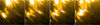 |
Fig. A.1 Example of the frame-by-frame tracking procedure. The dark blue squares indicate the manually identified front of the downflow in successive frames, while the black dashed line in the last panel indicates the manually measured length of the downflow. |
All Figures
|
Fig. 1 Overview of the positions (a) and viewing geometry from Solar Orbiter (b), and SDO (c). The cyan square denotes the field of view (FoV) of HRIEUV. Since the HRIEUV FoV partially lies outside the solar disk, we define a smaller on-disk region (green square) within the FoV and re-project this region onto the SDO perspective. |
| In the text | |
|
Fig. 2 Overview of the downflows in this event. Panel (a) shows the field of view of the HRIEUV observation. The boxes labelled R1 and R2 mark two different flare-ribbon regions. Panels (b) and (c) present zoomed-in views of regions R1 and R2. Panels (b1–b4) and (c1–c4) display the detailed temporal evolution of two selected individual downflows. The fields of view of these panels are indicated by the black squares in panels (b) and (c), respectively. The blue arrows indicate the trajectories of the downflows. The pink and cyan arrows mark the locations of the downflows in the corresponding frame. (An online animation is available for this figure.) |
| In the text | |
|
Fig. 3 Overview of the same active region as in Fig. 2, observed with SDO/AIA 171 Å and 1600 Å at four different times. The pink and cyan arrows mark the same locations as in Fig. 2. |
| In the text | |
|
Fig. 4 Temporal evolution of Region 2 observed by EUI and the SXR and HXR emission of the flare. Panels (a)–(d) show the evolution of Region 2, while panel (e) displays the GOES 1–8 Å SXR light curve together with the STIX 4–10 keV and 25–50 keV HXR light curves. Details of the HXR data processing are described in Tan et al. (2025a). The grey shaded region indicates the EUI observing time span. The vertical dashed lines mark the times corresponding to panels (a)–(d). |
| In the text | |
|
Fig. 5 Histograms of the statistical properties of the downflows identified in Region 1 and Region 2. The values marked in each panel indicate the corresponding mean values. The starting time in panel (d) corresponds to the first appearance of the downflow. |
| In the text | |
|
Fig. 6 Cartoon scenarios of the observed downflows. The five-pointed star symbol indicates the magnetic reconnection site. This sketch is adapted from Lysenko et al. (2020). |
| In the text | |
|
Fig. A.1 Example of the frame-by-frame tracking procedure. The dark blue squares indicate the manually identified front of the downflow in successive frames, while the black dashed line in the last panel indicates the manually measured length of the downflow. |
| In the text | |
Current usage metrics show cumulative count of Article Views (full-text article views including HTML views, PDF and ePub downloads, according to the available data) and Abstracts Views on Vision4Press platform.
Data correspond to usage on the plateform after 2015. The current usage metrics is available 48-96 hours after online publication and is updated daily on week days.
Initial download of the metrics may take a while.