| Issue |
A&A
Volume 709, May 2026
|
|
|---|---|---|
| Article Number | A177 | |
| Number of page(s) | 14 | |
| Section | Astronomical instrumentation | |
| DOI | https://doi.org/10.1051/0004-6361/202659395 | |
| Published online | 13 May 2026 | |
Simulations of a 2 × 1.5D coded aperture camera for X-ray astronomy
1
SRON Space Research Organization Netherlands,
Niels Bohrweg 4,
2333 CA
Leiden,
The Netherlands
2
INAF-IAPS Roma,
via Fosso del Cavaliere 100,
00133
Rome,
Italy
3
Institute of Space Sciences (ICE-CSIC),
Campus UAB,
08193
Cerdanyola del Vallès (Barcelona),
Spain
4
Institut d’Estudis Espacials de Catalunya (IEEC),
Barcelona,
Spain
★ Corresponding author: This email address is being protected from spambots. You need JavaScript enabled to view it.
Received:
10
February
2026
Accepted:
16
March
2026
Abstract
The concept of two perpendicular, 1D coded aperture cameras, necessitated by the imaging capability of the detector, is applied in the design of the Wide Field Monitor (WFM). The goal of this instrument is to monitor the variable X-ray sky for transient activity. Each camera features a fine angular resolution in one direction (typically 5 arcmin) and a coarse one in the other (5 degrees). The coarse perpendicular resolution makes the camera “1.5D”. The WFM has been studied for a number of space-bound X-ray observatory concepts: the Large Observatory For Timing (LOFT), the enhanced X-ray and Timing Polarimetry mission (eXTP), the Spectroscopic Time-Resolving Observatory for Broadband X-rays (Strobe-X), the Astrophysics of Relativistic Compact Object mission (ARCO), and now the Lunar Electromagnetic Monitor in X-rays (LEM-X). We report a study of two decoding algorithms for this instrument and its imaging performance. Detector responses to the X-ray sky are simulated, including the signal processing. The decoding algorithms are the iterative removal of sources (IROS), in combination with cross-correlation, and the maximum-likelihood method (MLM). IROS is most suited to the determination of the point-source configuration of the observed sky and MLM for the optimum determination of the source fluxes. The simulation results show that despite the 1.5D imaging of each camera, the reconstruction of scientific data is as if each camera pair were replaced by a single 2D camera with the same angular-resolution specification and a detector size equal to that of the two in the pair, except that source confusion is somewhat higher in the former. Thus, the WFM is a high-performance monitoring instrument with straightforward and proven technology that enables the identification of new cosmic X-ray sources, like X-ray novae, gamma-ray bursts, electromagnetic counterparts to gravitational-wave events, and interesting behavior of persistent X-ray sources, like accretion-disk state changes.
Key words: instrumentation: miscellaneous / methods: numerical / techniques: image processing / telescopes
© The Authors 2026
 Open Access article, published by EDP Sciences, under the terms of the Creative Commons Attribution License (https://creativecommons.org/licenses/by/4.0), which permits unrestricted use, distribution, and reproduction in any medium, provided the original work is properly cited.
This article is published in open access under the Subscribe to Open model. This email address is being protected from spambots. You need JavaScript enabled to view it. to support open access publication.
1 Introduction
Apart from rotation, the sky seems static to the naked eye, but this is far from true. Particularly in X-rays, it is vibrant, with variability and transient activity on all timescales. This became clear early in the 1960s with the dawn of X-ray astronomy through instrumentation specifically designed for detecting transient activity on Earth (atmospheric nuclear weapons tests) through the Vela satellites (e.g., Klebesadel et al. 1973). This motivated the implementation of a long series of X-ray all-sky monitors (ASMs) throughout history, the most recent examples being the Monitoring All-sky X-ray Imager (MAXI) launched in 2009 to the International Space Station (ISS; Matsuoka et al. 2009), the cubesats Ninjasat (Tamagawa et al. 2025) and Black-cat (Falcone et al. 2024), the Wide Field X-ray Telescope (WXT) on the Einstein Probe (EP) launched in 2024 (Yuan et al. 2022), and the Ensemble de Caméras à LArge champ sur Interféromètre Réparti en Scintillateurs (ECLAIRs) on the Space Variable Objects Monitor (SVOM; Godet et al. 2014; Givaudan et al. 2024), also launched in 2024. This will continue in the future. The modernization of the ASM fleet concentrates on the extension of the bandpass to longer wavelengths than the classical X-ray regime (i.e., >1 nm) and higher sensitivity and higher duty cycles (i.e., larger fields of view); it thus collects larger exposure times per point on the sky per day. Reaching larger fields of view is accomplished by coded aperture imaging, a technique applied since the late 1970s and currently widely used through, for instance, the Burst Alert Telescope (BAT) on the Swift satellite (Barthelmy et al. 2005) and ECLAIRs; time multiplexing, such as in MAXI; and lobster-eye optics, a technique that has only been applied for a few years through the Lobster Eye Imager for Astronomy (LEIA; Zhang et al. 2022) and WXT. Coded aperture imaging (Dicke 1968; Ables 1968) is a relatively simple and low-cost technique. Although it is less sensitive than direct focusing techniques by a few orders of magnitude, it is sensitive enough to detect many interesting transients in our own galaxy (e.g., accreting stellar black holes, thermonuclear flashes on neutron stars, and stellar flares) and beyond (e.g., gamma-ray bursts). This technique has therefore been very successful.
Coded aperture cameras (for reviews, see Caroli et al. 1987; in’t Zand 1992; Skinner 2008; Braga 2020; Goldwurm & Gros 2022) are usually based on a planar detector with identical spatial resolutions in both dimensions, yielding identical angular resolutions in those dimensions. This is a convenient setup. However, this is not strictly necessary. For example, the Super-AGILE instrument on the Astro-Rivelatore Gamma a Immagini LEggero satellite (AGILE; Feroci et al. 2010; Evangelista 2010) consisted of two pairs of identical cameras with each camera having a high resolution in only one dimension and a coarse resolution in the other. By co-aligning both cameras to the same field of view (FOV), but orthogonally with respect to each other, the 1D cameras accomplish a high angular resolution in both dimensions. This more involved setup was necessitated by the 1D nature of the silicon microstrip detectors, but it also has a number of advantages in terms of weight and power consumption. The present paper concerns an instrument concept similar to that of SuperAGILE, but involving better performing silicon drift detectors (SDDs) and more pairs of orthogonal cameras to increase the FOV. It is called the Wide-Field Monitor (WFM). While other WFM publications focus on the hardware implementation of this instrument, we here focus on the principles of the software implementation: the development of an image and spectral-reconstruction algorithm customized for the pair of coded aperture camera setup, the investigation of the performance with these algorithms, and a comparison with a would-be 2D setup. This paper focuses on principles and first-order assessments of performance, and as such it is a state-of-the-art study. In the future, software development needs to continue and simulations need to reach a higher level of fidelity, ultimately culminating in analysis software for real data.
After introducing the WFM in more detail in Sect. 2, we summarize decoding algorithms both in general and specifically for the WFM in Sect. 3. In Sect. 4, we explain how we approached the simulations of the sources, background, and the instrument response. In Sect. 5, we discuss the simulation results of the images and what this says about the performance of the WFM; in Sect. 6, we discuss the spectral simulations. We end in Sect. 7 with the conclusions of our study and the way forward with regards to the treatment of WFM data once the instrument is launched.
Specifications of WFM relevant for imaging.
2 The Wide Field Monitor
The concept of the WFM instrument was conceived one and a half decade ago and first applied in the proposal for the Large Observatory For Timing (LOFT; Feroci et al. 2012; Brandt et al. 2014), followed by concept studies for the enhanced X-ray Timing and Polarimetry mission (eXTP; Zhang et al. 2019; Hernanz et al. 2018, 2022, 2024; Zwart et al. 2022), the Spectroscopic Time-Resolving Observatory for Broadband X-rays (STROBE-X; Ray et al. 2024; Remillard et al. 2024), the Astrophysics of Relativistic Compact Object mission (ARCO) submitted to the call for F3 mission concepts for ESA in 2025, and the Lunar Electromagnetic Monitor in X-rays (LEM-X; Del Monte et al. 2024). It is an array of wide-field cameras for monitoring transient activity in the X-ray sky at photon energies between 2 and 50 keV. The FOV of each camera is 20% of the full sky, and an array therefore enables exceptionally high duty-cycle monitoring. The instrument consists of N pairs of orthogonal 1D coded aperture cameras. They are often referred to as 1.5D cameras because the SDDs have a resolution, albeit coarse, in the perpendicular dimension (e.g., Hernanz et al. 2018). Table 1 summarizes the characteristics of one WFM camera as designed for eXTP. A prototype of such a camera is currently under construction at ICE-CSIC (Barcelona).
Each WFM camera hosts 2 × 2 SDDs in one detector plane that have a high spatial resolution in one direction and a coarse resolution in the other (see Fig. 1). Each of the four detectors has a sensitive area of 6.5 × 7.0 cm2. The 2 × 2 detector array is inter-spaced by 1.3 cm along the coarse direction and 2.8 cm along the fine direction. This space is a dead area in the detector plane. The detector plane is sensitive within a 15.8 × 15.3 cm2 boundary. A coded mask of 26.0 × 26.0 cm2 is 20.29 cm above the detector plane. The mask pattern thus consists of 1040 × 16 elements of 0.025 × 1.64 cm2 after ignoring the first and last ribs (see below) covering 26.0 × 26.0 cm2 (here, X is assumed along the fine direction and Y along the coarse). The space between mask and detector plane is shielded by a collimator to prevent photons from reaching the detector without passing through the mask. Each camera has a FOV of 90 × 90 square degrees of which the central 29 × 29 square degrees illuminate the full detector array (with part of the mask) and is (somewhat confusingly) called the “fully coded” field of view (FCFOV). The optical design of the camera remains unchanged since 2010 (e.g., Donnarumma et al. 2012; Brandt et al. 2014). To produce a setup with equal high angular resolution in both dimensions, each camera is paired with an identical camera rotated by 90 degrees along the optical axis. The ultimate WFM configuration consists of N pairs of cameras, each pointed at a different position on the sky. In LOFT, N=4, in eXTP N=3 (see Fig. 2), in STROBE-X N=4, in ARCO N=1, and in LEM-X N=7.
The mask pattern is based on a cyclic difference set from biquadratic residues of primes v = 4x2 + 1 with x odd (theorem 5.16 in Baumert 1971; see also Gottesman & Fenimore 1989), where the set elements are j =mod(i4,v) for i = 1..v. This yields that 25% of the numbers between 1 and v are a member. At those positions the mask pattern is defined as open, and at all the others it is closed. For the mask in the WFM, v was chosen to be 16 901 (x = 65). This mask pattern is folded in two dimensions over a 1040 × 16 array of 0.25 mm × 16.4 mm elements with the last 261 members of the biquadratic residue set not used. The mask incorporates 2.4 mm closed ribs within the 16.4 mm long slits, so the effective open area of the mask becomes 21.6%; see Fig. 3.
The WFM is, as all coded aperture cameras (and perhaps even more so because of its 2 × 1.5D nature), an indirect-imaging instrument. In contrast to focusing telescopes, the signal of all cosmic sources is coded and mixed, which gives rise to the disadvantage that there is cross talk between sources and decreased sensitivity for the same photon-collecting area. An essential ingredient of a coded aperture camera is the algorithm to decode the signal from the coded detector domain to the decoded sky domain. The purpose of the present paper is to discuss methods to treat the data through such algorithms and verify through detailed simulations the expected performance.
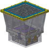 |
Fig. 1 WFM camera shown with the shielding made slightly transparent. In purple, the four SDDs are depicted; the mask is shown on top. |
3 Algorithms to decode detector data into sky data
Various successful algorithms to accomplish the reconstruction of sky data from coded aperture detector data are discussed in the literature (e.g., Rideout 1995). This includes cross-correlation (Brown 1974; Fenimore & Cannon 1978), the maximum-likelihood method (MLM; Skinner & Nottingham 1993; Nottingham 1993), the maximum-entropy method (Willingale 1981), Wiener filtering (Sims et al. 1980; Rideout & Skinner 1996), and machine-learning techniques (Meißner et al. 2023). The cross-correlation method has been extended with iterative removal of sources (IROS; Hammersley 1986; Hammersley et al. 1992; in’t Zand 1992), fine sampling, and delta decoding (Fenimore & Cannon 1981). We developed the IROS method and the MLM for application in the WFM. These methods have different purposes. IROS excels in fast sky-image reconstruction and searches for previously unknown point sources. The MLM excels in the best determination of fluxes and positions. IROS provides a map of the complete FOV by the fast cross-correlation technique using FFTs. The MLM can provide a sky map by calculating detector images for every possible sky location, which is a slower process. Our approach to the handling of WFM data is to first find all point sources through IROS and then characterize all those point sources (i.e., determine positions, light curves, and spectra) through the MLM.
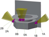 |
Fig. 2 A schematic of the WFM configuration foreseen for eXTP as an example. The narrow-field instruments of eXTP are pointed upward, so the WFM pair “0” covers the pointing of those instruments at the center of the FOV. |
3.1 Iterative Removal of Sources
3.1.1 Outline
Iterative Removal Of Sources is an analog of the “clean” algorithm in interferometric radio-astronomy imaging (Högbom 1974). The basis of IROS (Hammersley 1986) is a cross-correlation of the detector image with a mathematical version of the mask pattern that ensures the expected flux at any pixel where there is no source is zero and is properly normalized to phot s−1 cm−2 for any source pixel. The geometrical response of the instrument needs to be taken into account to properly normalize by cm2, for instance obscuration by support structures of the detector or mask. Any photon energy-dependent response parameters of the instrument – such as detector spatial resolution, mask transparency, and shadowing – need to be taken into account through, for example, modeling of the point-spread function (PSF) in the sky and detector domains.
A typical feature of cross-correlation images is “coding noise”. Mask patterns are chosen such that their autocorrelation is a delta function (Palmieri 1974; Fenimore & Cannon 1978). This requires the application of patterns based on pseudo-random arrays, such as cyclic difference sets, and the proper folding of a 1D array in 2D. Figure 3 shows the mask pattern of the WFM envisaged for eXTP. Even with a pseudo-random pattern, the autocorrelation is only two-valued if the full pattern is involved in coding any sky position. There are some camera configurations with which this has been accomplished, for instance by applying a repeated ideal mask pattern and putting a collimator on the detector that limits the FOV from any position on the detector to one complete cycle of such a pattern (Hammersley 1986). However, in many practical applications (e.g., when sensitivity or FOV is critical) this is not the case, and coding noise is present, with a variance that is proportional to the portion of the basic pattern not used in coding a sky position. This also pertains to the WFM. The mask pattern is larger than the detector, so it is never completely recorded. The portion of the FOV that uses the complete detector we call the FCFOV. However, in the WFM this is actually not coded with the complete mask pattern, so it has coding noise. Outside the FCFOV only part of the detector is illuminated, and the coding noise becomes worse, although less so than for a random mask pattern. Generally speaking, the local coding noise standard deviation is a fraction of the random case that is equal to the square root of the fraction of the mask pattern employed in coding that locality. Ergo, we expect the base level of coding-noise standard deviation to be  of that for a random mask pattern, with NSSD = 4 being the number of SDDs, ASDD = 6.5 × 7.0 cm2 the sensitive area per SDD, and Amask = 26.0 × 26.0 cm2 the area of the mask. The expression under the square root represents the minimum fraction of the complete mask pattern not used during the coding of a sky source. Coding noise is a systematic and deterministic noise, meaning that it does not diminish with exposure time as opposed to statistical noise. However, one can eliminate or minimize it with IROS. IROS entails the following critical steps (see also Fig. 4):
Cross-correlate the detector image with a mathematical version of the mask pattern of a sky image – properly normalized so that each pixel has phot s−1 cm−2 as unit – and an accompanying error image of the statistical standard deviation in each pixel based on Poisson photon-count statistics (see, e.g., in’t Zand 1992).
Identify significantly detected point sources in the cross-correlation image where significance is determined with respect to the local image’s standard deviation after a PSF fit that yields their fluxes (e.g., in’t Zand et al. 1994).
Model the detector image for these point sources and exposure time.
Subtract the model detector from the observed detector image.
Cross-correlate the residual detector image with a mathematical representation of the mask pattern into a sky image. The sky image will still have systematic biases because the initial flux determination is subject to coding noise, but the coding noise will be smaller than after the previous iteration.
Go back to step 2 while preserving the original error image and iterate until there are no more significant point sources remaining.
Re-introduce the PSF models of all iterations and sources back in the last cross-correlation image and perform a PSF fit to determine the best-estimate fluxes.
The convergence of the iterative process of IROS can be significantly improved if one takes into account the knowledge about known point sources in the FOV; that is, in other words, if one uses an X-ray catalog and the accurate pointing direction of the camera (usually provided by optical star trackers on board). After all, the known point sources concern the brightest sources, except for an incidental new transient, and are the dominant source of coding noise. Furthermore, one can keep the positions of these frozen during the PSF fits. Freezing the positions of the bright sources leaves fewer parameters to fit and eases the iteration process, particularly in crowded fields (likely in wide-field applications) because the coding noise can become large. If there is no pointing information available or its accuracy is compromised, the camera’s X-ray data can be used for plate-solving constellations of X-ray stars, and pointing information can be recovered.
In IROS, we chose to fit the model to the data in the sky domain. Alternatively, one could do this in the detector domain, but in principle this does not matter as the translation of detector data into sky data is a cross-correlation procedure that is a linear combination of detector data into sky data; this is independent for every sky pixel.
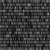 |
Fig. 3 WFM mask. The cyclic difference set is laid down starting from the bottom left, going first from left to right and then bottom to top. |
3.1.2 Implementation
We list the particularities of our implementation of IROS for the WFM below.
The WFM data are provided on an event-by-event basis and include positions with a readout accuracy that is a fraction of the 60 µm fine resolution. We chose to bin these data to detector bins of 0.25 mm × 0.25 mm, which is commensurate with the fine mask-element size, yielding a total detector image size of 632 × 632 pixels (filling up dead areas between SDDs or along their edges with zeros to obtain paired detector images for X and Y cameras) and a sky image size of 1671 × 1671 pixels.
The cross-correlation images of the X and Y cameras are added in step 1, resulting in a cross-like PSF that is fit to simultaneously obtain accurate estimates for locations in X as well as Y and flux in step 2, while the treatment of the detector images of X and Y in steps 3 and 4 remains separate. Thus, uncertainty about the coarse position of each source can be avoided, and the iterative process is more efficient.
If in step 3 the center of the PSF of one source is on the PSF of another, only the most significant source is included in the current iteration. In a subsequent iteration, the ignored source will likely be the most significant one.
If a source was “subtracted” in a previous iteration, negative fluxes are allowed to be subtracted if they are significant. This corrects possible overestimates of the flux in a previous iteration (due to coding noise).
The PSF looks as in Fig. 5. Due the shadowing by the mask thickness (150 µm) for an off-axis source, the PSF along the fine direction in particular has a plateau that depends on the off-axis angle and is off-centered. Since we chose to use 0.25 mm × 0.25 mm, there is no oversampling, which in principle introduces ambiguity in source positions; however, this can be avoided by fixing the point source locations (except for unknown sources) and oversampling in the MLM to accurately determine the position of new sources.
It is noted that IROS can be run independently on the X or the Y camera. The sensitivity decreases by a factor of  , and the source confusion increases along the coarse direction, but a high level of redundancy is preserved. Something similar happens for the multiple detectors in one detector plane.
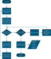 |
Fig. 4 Flow diagram of IROS. |
3.1.3 Verification
One step in IROS is the calculation of the model detector image for a given source configuration (step 3). This is done through a geometric calculation of the projection of the mask on the discretized detector. This analytical step enabled us to verify the self-consistency of IROS: what one puts in should come out. This implies that source fluxes should be reproduced exactly and the standard deviation of any reconstructed sky image after source subtraction should be zero since no count statistics are involved. We first tested this with just a single point source and then in the most complicated sky configuration possible, namely that of the Galactic center (GC) field.
The test for the single point source was done in various positions in the FOV and was ideal every time (standard deviation zero). For the GC field, this is not the case. We find that IROS is able to diminish the standard deviation of the full significance image without point sources generally to 1–10% of the value that would be expected from Poisson noise for a 10 ksec exposure, or equivalent to the Poisson noise for a 1 Ms exposure of the GC. Figure 6 shows the results in terms of standard deviation of significance images for 658 different observation pointing realizations.
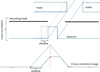 |
Fig. 5 PSF formation along the “fine” direction. In the top section of the figure, the rays of an off-axis source illuminate the thick mask somewhat sideways and introduce a shadow on one side of the projection of the mask element on the detector (middle blue graph). When cross-correlating with the decoding mask (moving the decoding mask from left to right over the detector; see middle blue graph), this introduces (bottom blue graph) (1) a flat top to the PSF which is off-centered; (2) a lower PSF peak representative of a less sensitive area; and (3) a narrower PSF. The red dots indicate where the discrete cross-correlation would sample the PSF if the sampling is equal to the mask element size. The sampled cross-correlation looks like there is no shadowing, but its integral is actually smaller. |
3.2 Maximum-likelihood method
3.2.1 Outline
Once all sources of detector events have been identified, in other words once all point and extended sources have been localized and the backgrounds calibrated, it may become desirable to apply further diagnostics on the sources: determine the time history of the fluxes (i.e., the light curves) and measure the spectrum, if need be, as a function of time or phase. This implies determination of source fluxes at many times and photon energies. In principle one can run IROS for every time and energy bin and keep source positions fixed, but this will require many computations and long processing times. This is basically because with IROS the flux is calculated in each of the almost 3 million sky pixels (in our WFM application), while one only needs the flux for around 100 sources. Therefore, one should resort to a method that is better suited, and that method is the MLM.
In the MLM, the measured detector image Di (in units of event counts per detector bin) for a given measured energy band is compared to a theoretical model consisting of a background component (or multiple background components, not considered here) and a combination of Nsrc point sources at different sky locations, all with free scale factors and taking into account the Poissonian nature of the counting process. Optimizing these scale factors by maximizing the likelihood ℒ gives the source strengths and associated uncertainties of the involved sources as well as an estimate for the background plus its uncertainty. In detail, for detector bin i we can write the expectation value Ei as
 (1)
(1)
where Mij is the PSF at that detector bin, i, for source j; Sj the source flux in sky bin j; Bi the background image in detector bin i; and β the scale factor of the total background component. The likelihood ℒ, taking into account the Poisson statistics, is defined as
 (2)
(2)
Assuming for simplicity that we are dealing with one source and one constant background model, Bi, ignoring times when the Earth eclipses part of the FOV, we consider two hypotheses: a) the zero hypothesis, ℋ0, stating that the data are described by background only (i.e.,  ), and we have
 (3)
(3)
and b) the alternative hypothesis, ℋ1, stating that the data are described in terms of a constant background and a point-source (i.e.,  ), resulting in
 (4)
(4)
Maximizing the natural logarithm of  with respect to β and S 1 and the natural logarithm of
  with respect to β, we can define the maximum-likelihood ratio (MLR), Q, as
 (5)
(5)
This (test) statistic is successfully used in high-energy astrophysics, particularly in the gamma-ray domain, for parameter optimization and hypothesis testing. More information on the basic principles, the method, and caveats can be found in Wilks (1938), Eadie et al. (1971), and Cash (1979), while its application to high-energy data analysis procedures is described in detail in Pollock et al. (1981), Mattox et al. (1996), de Boer et al. (1992), and Abdo et al. (2009) for the Cosmic Ray Satellite “option B”, the Energetic Gamma-Ray Experiment Telescope and the Compton Telescope on the Compton Gamma-Ray Observatory, and the Large Area Telescope on the Fermi Gamma-Ray Space Telescope, respectively. An application of the method to the Giuseppe “Beppo” Occhialini Satellite per Astronomia a raggi X (BeppoSAX) X-ray data is given in in’t Zand et al. (2000).
In our case the quantity Q is distributed as χ2 for one degree of freedom under proper conditions. Therefore, at known source locations (e.g., from source catalogs) Q values of 9, 16, 25, and so on correspond to 3σ, 4σ, 5σ, and so on detection significances.
If we do not know, a priori, the location of a source, we can scan the sky on a grid by assuming a source location at each grid point and evaluate the quantity Q, thus constituting a map (i.e., the MLR significance map). To assess the significance of prominent new-source features in the MLR map we have to take into account the number of trials; that is, the number of independent spatial-resolution elements (∼4′×4′) searched for in the map, which degrades the detection significance compared to the assumption of the one degree-of-freedom significance at the particular location. The construction of this map is a tedious and CPU-time-consuming process given the nonlinear nature of the optimization procedure and the many scan locations (preferentially sampled at step sizes smaller than the angular resolution of the camera) involved to build the map, requiring a different detector model each time. This procedure is feasible as long it is limited to a small region around a new source for the sake of its identification, but the computations quickly become unsustainable for a large FOV. Appendix A shows an example of a subregion of the WFM FOV.
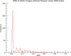 |
Fig. 6 Histogram of standard-deviation values of significance images of the GC field solution without Poisson noise for 658 different pointings (i.e., rotating from 0 to 359 deg in steps of 1 deg and for stepping diagonally over the image in 299 steps at one rotation angle). |
3.2.2 Implementation
The practical implementation is as follows. At first, the events in the detector plane (for a measured energy band) are binned in 30 µm by 3.5 mm detector pixels along the fine and coarse directions, respectively, which is sufficiently small to sample sufficiently dense the 60 µm and 8 mm FWHM resolution in the fine and coarse directions of the detector. This results in a 2170 × 20 binning mesh per detector plane given its (X,Y) sizes. This detector image is denoted by Di.
The next step is to accurately determine the pixel illumination factor (PIF) for each pixel in the detector plane for a given source scan direction. For this purpose we subdivided each detector pixel into M × M elements to boost the detector image resolution and determine whether the (centers of) these elements are blocked by a mask element or not when back projecting to that source in the sky. M is typically 3. We performed this procedure for both the upper and lower mask plane (the mask is 150 µm thick). The current implementation yields a 1 or 0 for an open and blocked element, respectively. In principle, the method can include energy-dependent absorption effects (the mask is more opaque at lower X-ray energies) by the Tungsten mask elements using the measured energy of the events as a proxy for the photon energy, yielding fractional values between 0 and 1.
We also took into account the averaged penetration depth, dpen, of the photons in the silicon detector material, effectively making the detector–mask distance larger by dpen. Finally, we blurred it through convolution of the detector image, as derived above for the case in which we know the (X, Y)-location of the absorbed photon in the detector plane precisely, with a 2D-distribution that accurately describes the blurring of the charge cloud reconstruction produced by the absorbed photon. This description is a “modified” sech(x) function (secans hyperbolicus) of the form
 (6)
(6)
where x is the spatial dependence and a is a four-element parameter array describing the model PSF. Only the “shape” parameters, a2 and a3, are relevant for the normalized distribution used in the convolution process. Thus, we have the necessary elements: (a) the measured detector Di; (b) the PSF Mij for a source at the scan location; and (c) a background estimate assumed to be homogeneous for isotrope diffuse emission to calculate the maximum likelihood ratio, Qk, for each scan location, k. The square root of this number yields the significance image.
Due to the additive nature of lnℒ (i.e., the multiplicative character of the likelihood ℒ), the method can easily be extended to analyze an orthogonal camera pair assuming that both components are identical and operate simultaneously under similar observation conditions. In that case, we can assume that the same fit (scale) parameters for the models hold for each component of the camera pair. In practice, one should correct for possible slightly different exposure times and misalignments of each camera.
4 Simulation approach
4.1 Simulation of sky
Our baseline for the simulation of point sources is the catalog of cosmic X-ray point sources, as compiled from observations with the Bruno Rossi X-ray Timing Explorer (RossiXTE) ASM (Levine et al. 1996, 2006, 2011) and BeppoSAX Wide Field Camera instrument (WFC; Jager et al. 1997). This includes 1.5–12 keV photon fluxes of those point sources averaged over the 16 year lifetime of the RossiXTE mission (1996–2012), the best-known positions – often from optical or radio observations – and average spectra measured with BeppoSAX-WFC (Verrecchia et al. 2007). The fluxes were normalized to the flux of the Crab and then multiplied with its calculated photon flux expected in the WFM in the bandpass of 2–30 keV (2.4 phot s−1 cm−2 based on the Crab spectral model of Kirsch et al. 2005). It is noted that this is an educated estimate of those fluxes with an assumed accuracy of a few tens of percent, but this is enough for our purposes to assess the WFM imaging capability and sensitivity.
We simulated the sky background by calculating the detector response to an isotropic background. This local response of the detector depends on the FOV as seen from that position on the detector since the FOV can be modulated by shadowing with any mechanical structure above it, including the mask. Our simulation entails a calculation of that FOV and a scaling that is determined from a Monte Carlo simulation of the cosmic diffuse X-ray background (CXB), which is 215 phot s−1 cam−1 for the full bandpass and is in line with CXB model in Marshall et al. (1980). Apart from the sky background, real observations will also include particle-induced background (Campana et al. 2012) and the Galactic-ridge emission (Valinia & Marshall 1998). However, the photon rates of these contributions are expected to be less than 10% of the CXB and, hence, negligible at the current level of fidelity.
We employed two sky fields as test cases:
The faint field. This is pointed at the Large Magellanic Cloud, particularly the point source LMC X-1. The combined photon count rate of all point sources is smaller than the background. The typical flux of a bright source in this FOV is a few tens of mCrabs. The brightest object is Cen X-3 at 53 mCrab at an off-axis angle of 34◦. The CXB count rate encompasses 97.6% of the total and so is dominant.
The bright field, which is pointed at the GC. The combined photon count rate of point sources far exceeds that of the background. In particular, this field contains Sco X-1 at an off-axis angle of 24◦, which is 10◦ outside the FCFOV. The average count rate of Sco X-1 is 11 times higher than the next brightest source in the field, GX 5-1, which is at an off-axis angle of 5◦. This field is an excellent test of systematic errors in the reconstruction. The CXB count rate encompasses 19.7% of the total and, therefore, is of secondary magnitude.
4.2 Simulation of detector response
Simulations of the WFM detector response were calculated per (array of) cameras with the physics-based software tool “WFM Imaging Simulation Environment for Montecarlo and ANalytical modeling” (WISEMAN). This tool is comprehensively described in Ceraudo et al. (2024). We summarize it in the next section.
4.2.1 The simulation process
Photons from astrophysical sources (hereafter, primary photons) are generated in the FOV of the camera starting from the ASM catalog of X-ray point sources and the diffuse emission of the CXB. Extended sources such as the Galactic ridge, supernova remnants, and galaxy clusters are not included. Primary photons (tagged with celestial coordinates, photon energy, and time of arrival) are projected uniformly on the top surface of the camera, and their direction is converted to the local frame of reference.
The first loss of primary photons flux occurs above the mask, where the presence of the multilayer insulator (MLI) foil was simulated, with the photons surviving the passage according to a stochastic process based on the overall transparency of the MLI. Afterward, the trajectory of each photon was traced through the mask, and the path into each (portion of) closed element was recorded so that the transmission of each photon may be calculated via a random process. All surviving photons were then traced to the detector plane, via a polypropylene foil between the mask and detector plane, and only those whose trajectories intersected with the detectors were followed further.
If the photon survives the passage through the inert layers of the top of the sensor, the interaction of a photon with the sensitive bulk is evaluated according to its energy and the path it actually traces, which depends on its direction of approach. If the photon is absorbed via a photo-electric effect in the sensor, its energy is modified by the Fano noise in silicon, and then the drift of the liberated electrons is simulated. During the drift, the initially point-like charge cloud expands under the effect of diffusion, so the charge, ψi, collected by an anode in position xi is
![Mathematical equation: ${\psi _i} = {1 \over 2}E\left[ {{\rm{erf}}\left( {{{{x_i} + p/2 - X} \over {\sigma \sqrt 2 }}} \right) - {\rm{erf}}\left( {{{{x_i} - p/2 - X} \over {\sigma \sqrt 2 }}} \right)} \right],$](/articles/aa/full_html/2026/05/aa59395-26/aa59395-26-eq13.png) (7)
(7)
where p is the anode pitch (169 µm), X and Y are the coordinates of the interaction of the photon with the detector, E is its energy, and σ is the width of the charge distribution due to diffusion; this is expressed by
 (8)
(8)
with D the diffusion coefficient, t the drift time, σ0 the initial width of the charge cloud, T the detector temperature, µ the electron mobility, ϵ the electric field, q the elementary charge, and kB Boltzmann’s constant (Campana et al. 2011).
Readout is implemented by adding noise to each anode reading, converting the continuous energy values to the integer units of the analog-to-digital converter and adding channel-wise offsets as well as an event-dependent baseline.
The final step of the simulation essentially consists of estimating the parameters of the interacting photon (X, Y, and E) from the recorded list of digitized anode readings. This procedure involves the application of user-provided calibration tables (e.g., gain, offset etc.) as well as a fit of the recorded charge profile.
At the end of the simulation, an output file resembling the actual data stream of an operating instrument is provided, featuring the list of the inferred energies and impact (X, Y) positions of the photons.
4.2.2 Strengths and limitations
The WISEMAN simulator can be employed to estimate the scientific performances of an arbitrary arrangement of WFM cameras; hence, it is not limited to a specific configuration (e.g., LOFT, eXTP, STROBE-X, ARCO, or LEM-X). Moreover, since nearly every camera subsystem is implemented, parametric simulations can be performed to perfect the design as a function of geometry, building materials, general characteristics, and performances of the various components (e.g., electronic noise and defective readout channels).
Deviations from the ideal geometric configuration may also be investigated, since each subsystem may be freely positioned around its baseline location, allowing us to simulate 3D shifts and rotations of mask and detectors, and therefore their impact on the scientific performances of the instrument. Likewise, the sensitivity of the reconstruction algorithms to deviations from the baseline configurations that are unaccounted for may be assessed in this way.
At the current stage of development, the simulator features some limitations. For example, all primary photons (and associated detected events) are treated completely independently of each another, implying the impossibility to quantify such effects as pile up and dead time, although that is expected to be limited. Additionally, only photons from astrophysical sources are simulated, and their energy and direction stay constant until the final interaction with the detector: no particle background or particle-induced photon background are implemented, and primaries are not reprocessed via scattering. Likewise, events derived from electronic noise were not considered. Finally, as previously mentioned, the astrophysical photons sources are currently limited to point sources (provided via a catalog) and the CXB. No Galactic ridge has been included. Also, at the current stage of development, the model that is used for simulating input for the IROS tests assumes infinitely dense masks and detectors and real photon absorption positions. The algorithm to derive photon detector positions is not developed yet at a sufficiently high fidelity to avoid large-scale low-amplitude features in detector images that are noticeable in IROS images. For the MLM simulations, the model is sufficient and avoids these idealizations, because the focus there is on (spectra of) bright sources.
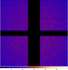 |
Fig. 7 Image of X detector (fine resolution along X) for LMC field for an observation with an exposure time of 10 ks. Unit is photon counts per 0.25 mm × 0.25 mm bin. The color-scale bar of the pixel values is shown at the bottom. The cross is due to the spaces between the four SDD tiles in the detector plane. |
5 Image simulations
5.1 IROS on the LMC field
The detector image of the WFM X camera of the simulated 10 ksec observation on the LMC is shown in Fig. 7. This simulation involves 2.7 million photons. It has the following features:
A thick, vertical running center bar and a thin horizontal one. This aligns with the spaces between the 4 SDDs. The space is larger in X because there is more hardware along those edges of the SDDs.
No obvious exposures of point sources, because their count rates are negligible with respect to that of the CXB.
A large-scale non-uniformity peaking at the center of the detector. This is due to the FOV as seen from the center of the detector being approximately 20% larger than from the corners.
The Y camera shows a similar detector image (not shown) but rotated by 90◦. The IROS solution of this observation is shown in Fig. 8, zooming in on 40% of the total image with the six most significant sources. The weakest source is LMC X-4 (not shown) at a significance of 3.1, suggesting a five-sigma detection limit of 7 mCrab for this field.
5.2 IROS on GC field
Figure 9 shows the detector image of the X camera for the 10 ks simulated observation of the GC. This measurement with the X camera includes 11 million photons, 21% from the CXB and 44% from Sco X-1 – the brightest point source in the FOV. The Y camera image (not shown) is similar. Many of the 163 catalog sources in the FOV leave photons on the detector.
This observation is in juxtaposition to the one on the LMC. It is dominated by the brightest point sources and as such represents the least sensitive field in the sky. This is clear from the detector image, which is dominated by the illumination by Sco X-1 at an off axis angle of 24◦. This illumination also clearly shows a shadowgram of the coded mask with the 14 mm long mask elements and the 2.4 mm ribs between them along the same axis. The CXB is not discernable, as opposed to the image of the LMC field (Fig. 7).
In Fig. 10, the IROS solution is shown for this observation. This 10 ksec observation reveals detections of 41 point sources. IROS is effective in that it brings down the overall standard deviation in the significance image down from 28 to 1.1, the large initial standard deviation being due to coding noise from mostly Sco X-1. After the first IROS iteration, involving only the subtraction of Sco X-1, the standard deviation already goes down to 6. The significance of Sco X-1 is very high at about 1400. The significance of a source very close to the GC, 1E1747.0-2942, is 2.3. This translates to a five-sigma sensitivity of 25 mCrab, which is roughly three times less sensitive than the faint LMC field, which therefore shows the dynamic range of sensitivities for any WFM observation within the same exposure time.
Sco X-1 is 24◦ from the GC. With a single camera pair FOV of 90 × 90 square degrees, it is cumbersome to keep Sco X-1 outside the FOV while keeping focused on the GC. It would imply that the GC needed to be placed some 25 degrees from the edge of the FOV, or 20–30 degrees from the center, depending whether it would be moved towards a corner or not. Since the FCFOV is the central 29 × 29 square-degree part of the camera field, the loss in detector area covering the GC would be limited to 15–30%.
The detrimental effect of Sco X-1 on the sensitivity was calculated by doing the same GC simulation while “turning off” Sco X-1. This shows a 40% improvement in the sensitivity of the 10 ksec GC observation for the on-axis position and less when far away from Sco X-1. Because Sco X-1 is outside the FCFOV, there are parts in the sky image opposite to where Sco X-1 resides that are not affected by the presence of Sco X-1, but the vast majority of the Galactic-bulge sources are within reach of the Sco X-1 cross talk. In Appendix B we show a simulation of a complete WFM instrument for the eXTP configuration (N=3) as an illustration.
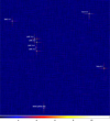 |
Fig. 8 Part of the sky image of the LMC observation as obtained through IROS, between –28◦ and +40◦ in the local frame along X and –39◦ and +25◦ in Y, zooming in on 40% of the total image (i.e., the fraction of sky pixels), showing the strongest sources in the FOV. The pixel unit is significance. Only sources brighter than 13 mCrab are labeled. The cross-like PSF of a source is not always apparent, because its narrowness is not clear at this image reproduction; it is clearer when zooming in on the pdf version of this paper. |
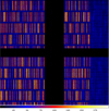 |
Fig. 9 Image of X detector for an observation of 10 ks exposure of GC field. The illumination by Sco X-1 is obvious. Unit is photon counts per 0.25 mm × 0.25 mm bin. |
5.3 Special test: imaging with 1 × 2D instead of 2 × 1.5D
In order to assess how the WFM 2 × 1.5D configuration compares to a 1 × 2D configuration with similar capabilities, we set up a simulation with a 2D camera that has twice the detector area, but an identical FOV and angular resolution to the 2 × 1.5D configuration. This implies a simple scaling of all linear sizes by a factor of  . The result is shown in Fig. 11. Essentially, the significances of all sources are similar as are the positional uncertainties for non-cataloged sources, but the source confusion in the 2 × 1.5D configuration is substantially worse if two sources are located on each other’s PSF cross, which extends over an ∼256 times larger part of the FOV. This is particularly relevant for faint transients in the the Galactic bulge.
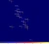 |
Fig. 10 Part of the sky image of the GC observation as obtained through IROS, between –44◦ and +45◦ in in the local frame along X and –35◦ and +35◦ in Y, zooming in on 70% of the total image (i.e., the fraction of sky pixels) showing the strongest sources in the FOV. The pixel unit is significance. Only sources brighter than 80 mCrab are labeled. The cross-like PSF of a source is not always apparent because its narrowness does not show well at this image reproduction; it is clearer when zooming in the pdf version of this paper. |
6 Spectral simulations
While IROS is most effective in image processing and will provide a complete list of point sources detected in the FOV with flux inferences at an accuracy typically up to a few percent (e.g., Goldwurm & Gros 2022), MLM, although also capable of producing images but at high CPU cost (see Appendix A), excels in the detailed analysis of those sources, in particular the determination of the high-resolution time history of their flux and their spectrum. We here show the spectral capability of MLM. One of the sources in the GC field, GRO J1655-40, is simulated with the following spectral ingredients that are inspired by the spectra of black-hole X-ray binaries in their hard state (e.g., see the review by Kalemci et al. 2022):
A continuum consisting of a power law with a photon index of Γ =1.86 and a normalization of 1.14 phot s−1 cm−2 keV−1 at 1 keV. This implies a brightness of 200 mCrab for this source, ignoring the line contributions specified below, which are substantially smaller.
Interstellar absorption with NH = 0.61 · 1022 cm−2 through the photoionization cross-sections of Verner & Yakovlev (1995) and Verner et al. (1996) and the abundances of Anders & Grevesse (1989).
A narrow Gaussian emission line at 6.4 keV with an intensity of 0.00263 phot s−1 cm−2. This line has an equivalent width of 60 eV.
A Laor emission line profile at 6.91 keV from an accretion disk surface with an emissivity dependence that is proportional to R−3, an inner radius of 1.235 GM/c2, an outer radius of 400 GM/c2, an inclination of the disk to the line of sight of 30 degrees, and an intensity of 0.0189 phot s−1 cm−2. This line has an equivalent width of 600 eV.
We applied the MLM to reconstruct the spectrum for GRO J1655-40 and model it with the four components mentioned above using XSPEC version 12.15.1 (Arnaud 1996) with the public response functions for the WFM. The result is shown in Fig. 12. We were able to reproduce the free model parameters as follows: NH = (1.63 ± 0.44) · 1022 cm−2 = +2.3σ, Γ = 1.90 ± 0.03 = +1.2σ, PL-normalization=1.268 ± 0.104 phot s−1 cm−2 keV−1 = +1.2σ, narrow Gaussian line E = 6.40 ± 0.08 keV=0.0σ, narrow Gaussian line intensity 0.0026 ± 0.0008 = −0.1σ, Laor line E = 6.90 ± 0.06 keV=−0.1σ, and Laor line intensity 0.0238 ± 0.003 phot s−1 cm−2 = +1.6σ. Therefore, the MLM reproduces the multicomponent spectrum of this 200 mCrab source accurately.
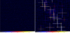 |
Fig. 11 Comparison of sky reconstructions of the GC field between the 2 × 1.5D configuration (right) and the 1 × 2D configuration (left), zooming in on the central quarter of the FOV. |
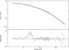 |
Fig. 12 Top panel: MLM reconstruction of the spectrum of GRO J1655-40 (data points) and best-fit model spectrum (drawn histogram). For details, see main text. Bottom panel: comparison between data points and model, after setting the normalizations of the two spectral lines to zero. |
7 Conclusion and future work
We developed and verified the performance of three independent software packages for application in the WFM: WISEMAN, to simulate the instrument complete signal chain from celestial X-ray sources to event data streams; IROS, to quickly and iteratively reconstruct the sky image from the coded detector data for a particular observation; and MLM, to quickly determine the fluxes for all X-ray sources in the FOV for any time interval within the observation and any photon energy interval. We find consistent results throughout, which supports the validation of all three software packages.
Experimentation with the software has shown that the concept of a pair of identical orthogonal 1.5D coded aperture cameras performs equally as well as one 2D coded camera of the same fine angular resolution, with the same FOV and an equal detector area to both 1.5D cameras combined, except for faint transients in the Galactic bulge. The advantages of this 2 × 1.5D setup are that it is possible to use lightweight, low-power consumption SDDs and that some level of redundancy is innate. The disadvantage is that the larger, cross-like PSF introduces an increased level of source confusion and cross talk between sources when they are on each other’s PSFs, but in the brightness range in which such a camera would be active, the source confusion is not a significant issue, except perhaps in the GC region.
Our work confirms, end-to-end, the feasibility of the WFM concept. Its modularity makes it easily adaptable to any mission or observatory concept, and it is low risk due to the implicit redundancy.
The simulation software makes it possible to test different configurations of the WFM and the mask pattern and vulnerability to imperfections such as slight misalignments between SDDs in one camera, the mask and detector plane, and the cameras in a pair. Regarding the latter, the independent functionality of a single camera comes in handy. Future work will focus on the verification of the alignment budget and experimentation with the mask’s pattern resolution to align with improvements in SDD spatial resolution, with timing resolution and with spectral resolution in the signal chain.
Acknowledgements
This work was performed by the eXTP-WFM Simulations Working Group that was active in 2020–2024 until the WFM instrument was removed from eXTP. Support was provided by INAF Rome, SRON and ICE-CSIC Barcelona. The employed software builds on earlier software written for missions BeppoSAX, AGILE, CGRO and INTEGRAL. We acknowledge all colleagues that were involved in writing the code. It is noted that no AI tool has been employed in the coding, data analysis or manuscript preparation.
References
- Abdo, A. A., Ackermann, M., Ajello, M., et al. 2009, ApJS, 183, 46 [NASA ADS] [CrossRef] [Google Scholar]
- Ables, J. G. 1968, PASA, 1, 172 [Google Scholar]
- Anders, E., & Grevesse, N. 1989, Geochim. Cosmochim. Acta, 53, 197 [Google Scholar]
- Arnaud, K. A. 1996, in Astronomical Society of the Pacific Conference Series, 101, Astronomical Data Analysis Software and Systems V, eds. G. H. Jacoby, & J. Barnes, 17 [NASA ADS] [Google Scholar]
- Barthelmy, S. D., Barbier, L. M., Cummings, J. R., et al. 2005, Space Sci. Rev., 120, 143 [Google Scholar]
- Baumert, L. D. 1971, Cyclic Difference Sets Braga, J. 2020, PASP, 132, 012001 [Google Scholar]
- Brandt, S., Hernanz, M., Alvarez, L., et al. 2014, SPIE Conf. Ser., 9144, 91442V [Google Scholar]
- Brown, C. 1974, J. Appl. Phys., 45, 1806 [Google Scholar]
- Campana, R., Zampa, G., Feroci, M., et al. 2011, Nucl. Instrum. Methods Phys. Res. A, 633, 22 [Google Scholar]
- Campana, R., Feroci, M., Del Monte, E., et al. 2012, SPIE Conf. Ser., 8443, 84435O [Google Scholar]
- Caroli, E., Stephen, J. B., Di Cocco, G., Natalucci, L., & Spizzichino, A. 1987, Space Sci. Rev., 45, 349 [Google Scholar]
- Cash, W. 1979, ApJ, 228, 939 [Google Scholar]
- Ceraudo, F., Evangelista, Y., Hernanz, M., et al. 2024, SPIE Conf. Ser., 13093, 130936T [Google Scholar]
- de Boer, H., Bennett, K., Bloemen, H., et al. 1992, in Data Analysis in Astronomy, eds. V. di Gesu, L. Scarsi, R. Buccheri, & P. Crane, 241 [Google Scholar]
- Del Monte, E., Ceraudo, F., Della Casa, G., et al. 2024, SPIE Conf. Ser., 13093, 130931U [Google Scholar]
- Dicke, R. H. 1968, ApJ, 153, L101 [Google Scholar]
- Donnarumma, I., Evangelista, Y., Campana, R., et al. 2012, SPIE Conf. Ser.,. 8443, 84435Q [Google Scholar]
- Eadie, W. T., Drijard, D., & James, F. E. 1971, Statistical Methods in Experimental Physics, 231 [Google Scholar]
- Evangelista, Y. 2010, PhD thesis, Universitá Degli Studi Di Roma ‘La Sapienza’ [Google Scholar]
- Falcone, A. D., Colosimo, J. M., Wages, M., et al. 2024, SPIE Conf. Ser., 13093, 1309317 [Google Scholar]
- Fenimore, E. E., & Cannon, T. M. 1978, Appl. Opt., 17, 337 [CrossRef] [Google Scholar]
- Fenimore, E. E., & Cannon, T. M. 1981, Appl. Opt., 20, 1858 [Google Scholar]
- Feroci, M., Costa, E., Del Monte, E., et al. 2010, A&A, 510, A9 [NASA ADS] [CrossRef] [EDP Sciences] [Google Scholar]
- Feroci, M., Stella, L., van der Klis, M., et al. 2012, Exp. Astron., 34, 415 [Google Scholar]
- Givaudan, A., Bégoc, S., Bertoli, W., et al. 2024, SPIE Conf. Ser., 13093, 1309370 [Google Scholar]
- Godet, O., Nasser, G., Atteia, J., et al. 2014, SPIE Conf. Ser., 9144, 914424 [Google Scholar]
- Goldwurm, A., & Gros, A. 2022, in Handbook of X-ray and Gamma-ray Astrophysics, eds. C. Bambi, & A. Sangangelo, 15 [Google Scholar]
- Gottesman, S. R., & Fenimore, E. E. 1989, Appl. Opt., 28, 4344 [CrossRef] [Google Scholar]
- Hammersley, A. 1986, PhD thesis, University of Birmingham [Google Scholar]
- Hammersley, A., Ponman, T., & Skinner, G. 1992, Nucl. Instrum. Methods Phys. Res. A, 311, 585 [Google Scholar]
- Hernanz, M., Brandt, S., Feroci, M., et al. 2018, SPIE Conf. Ser., 10699, 1069948 [Google Scholar]
- Hernanz, M., Brandt, S., in’t Zand, J., et al. 2022, SPIE Conf. Ser., 12181, 121811Y [Google Scholar]
- Hernanz, M., Feroci, M., Evangelista, Y., et al. 2024, SPIE Conf. Ser., 13093, 130931Y [Google Scholar]
- Högbom, J. A. 1974, A&AS, 15, 417 [Google Scholar]
- in’t Zand, J. J. M. 1992, PhD thesis, Netherlands Institute for Space Research [Google Scholar]
- in’t Zand, J. J. M., Heise, J., & Jager, R. 1994, A&A, 288, 665 [Google Scholar]
- in’t Zand, J. J. M., Kuiper, L., Amati, L., et al. 2000, ApJ, 545, 266 [Google Scholar]
- Jager, R., Mels, W. A., Brinkman, A. C., et al. 1997, A&AS, 125, 557 [Google Scholar]
- Kalemci, E., Kara, E., & Tomsick, J. A. 2022, in Handbook of X-ray and Gammaray Astrophysics, eds. C. Bambi, & A. Sangangelo, 9 [Google Scholar]
- Kirsch, M. G., Briel, U. G., Burrows, D., et al. 2005, SPIE Conf. Ser., 5898, 22 [NASA ADS] [Google Scholar]
- Klebesadel, R. W., Strong, I. B., & Olson, R. A. 1973, ApJ, 182, L85 [NASA ADS] [CrossRef] [Google Scholar]
- Levine, A. M., Bradt, H., Cui, W., et al. 1996, ApJ, 469, L33 [NASA ADS] [CrossRef] [Google Scholar]
- Levine, A. M., Bradt, H., Morgan, E. H., Remillard, R., & MIT/GSFC ASM Team 2006, Adv. Space Res., 38, 2970 [Google Scholar]
- Levine, A. M., Bradt, H. V., Chakrabarty, D., Corbet, R. H. D., & Harris, R. J. 2011, ApJS, 196, 6 [NASA ADS] [CrossRef] [Google Scholar]
- Marshall, F. E., Boldt, E. A., Holt, S. S., et al. 1980, ApJ, 235, 4 [NASA ADS] [CrossRef] [Google Scholar]
- Matsuoka, M., Kawasaki, K., Ueno, S., et al. 2009, PASJ, 61, 999 [Google Scholar]
- Mattox, J. R., Bertsch, D. L., Chiang, J., et al. 1996, ApJ, 461, 396 [Google Scholar]
- Meißner, T., Rozhkov, V., Hesser, J., Nahm, W., & Loew, N. 2023, J. Instrum., 18, P01006 [Google Scholar]
- Nottingham, M. R. 1993, PhD thesis, University of Birmingham [Google Scholar]
- Palmieri, T. M. 1974, Ap&SS, 28, 277 [Google Scholar]
- Pollock, A. M. T., Bignami, G. F., Hermsen, W., et al. 1981, A&A, 94, 116 [Google Scholar]
- Ray, P. S., Roming, P. W. A., Argan, A., et al. 2024, J. Astron. Telesc. Instrum. Syst., 10, 042504 [Google Scholar]
- Remillard, R. A., Hernanz, M., in’t Zand, J. J. M. et al. 2024, J. Astron. Telesc. Instrum. Syst., 10, 042505 [Google Scholar]
- Rideout, R. M. 1995, PhD thesis, University of Birmingham [Google Scholar]
- Rideout, R. M., & Skinner, G. K. 1996, A&AS, 120, 579 [Google Scholar]
- Sims, M., Turner, M. J. L., & Willingale, R. 1980, Space Sci. Instrum., 5, 109 [Google Scholar]
- Skinner, G. K. 2008, Appl. Opt., 47, 2739 [Google Scholar]
- Skinner, G. K., & Nottingham, M. R. 1993, Nucl. Instrum. Methods Phys. Res. A, 333, 540 [Google Scholar]
- Tamagawa, T., Enoto, T., Kitaguchi, T., et al. 2025, PASJ, 77, 466 [Google Scholar]
- Valinia, A., & Marshall, F. E. 1998, ApJ, 505, 134 [NASA ADS] [CrossRef] [Google Scholar]
- Verner, D. A., & Yakovlev, D. G. 1995, A&AS, 109, 125 [Google Scholar]
- Verner, D. A., Ferland, G. J., Korista, K. T., & Yakovlev, D. G. 1996, ApJ, 465, 487 [Google Scholar]
- Verrecchia, F., in’t Zand, J. J. M., Giommi, P., et al. 2007, A&A, 472, 705 [NASA ADS] [CrossRef] [EDP Sciences] [Google Scholar]
- Wilks, S. S. 1938, Ann. Math. Statist., 9, 60 [CrossRef] [Google Scholar]
- Willingale, R. 1981, MNRAS, 194, 359 [Google Scholar]
- Yuan, W., Zhang, C., Chen, Y., & Ling, Z. 2022, in Handbook of X-ray and Gamma-ray Astrophysics, eds. C. Bambi, & A. Sangangelo, 86 [Google Scholar]
- Zhang, S., Santangelo, A., Feroci, M., et al. 2019, Sci. China Phys. Mech. Astron., 62, 29502 [Google Scholar]
- Zhang, C., Ling, Z. X., Sun, X. J., et al. 2022, ApJ, 941, L2 [Google Scholar]
- Zwart, F., Tacken, R., in’t Zand, J. J. M., et al. 2022, SPIE Conf. Ser., 12181, 1218167 [Google Scholar]
Appendix A MLM on GC field
MLM can be employed to generate images. An example is shows in Fig. A.1, for part of the GC sky image. For this exercise, GX 5-1 was included in ℋ0 and the image was generated by scanning the FOV for deviations from ℋ0. As said, this is a computationally intensive exercise. The generation of this image, which covers only 8% of the FOV, took approximately 24 hr on a Linux Debian system with a 12th generation Intel(R) Core(TM) i7-12700K CPU.
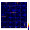 |
Fig. A.1 MLM solution of the central 25 × 25 square degrees of the GC observation, projected on an R.A.-Decl. plane (Eq. 2000.0). Sources are 4U 1820-30 at (R.A., Decl.)=(275.9,-30.4), GX 9+1 at (270.4,-20.5), GX 3+1 at (267.0,-26.5), GX 9+9 at (262.2,-17.0), GX 13+1 at (273.6,-17.2), GX 354-0 at (263.0,-33.8), GX 349+2 at (256.4,-36.4) and partially GRO J1655-40 at (353.5,-39.8). GX 5-1 is missing at (270.3,-25.1) because it is included in ℋ0. The pixel scale is Q (proxy for significance). |
Appendix B Complete eXTP-WFM simulation
In order to show what the potential is of a complete WFM instrument, we have simulated an observation centered close to the GC (i.e., GX 3+1) for the Sun position on March 15 for 3 camera pairs as would have been applicable for eXTP. The IROS solution is shown in Fig. B.1. This single observation covers the Galactic plane between −100 and +100 degrees in Galactic longitude and a substantial range of latitudes above and below the plane. It covers 40% of the sky (5.0 sr). It also covers 75% of all RossiXTE ASM sources and bright Galactic X-ray sources and 83% of all bright ASM sources (i.e., with an average flux higher than 10 mCrab). There are a few sources which are in overlapping FOVs of 2 adjacent camera pairs. These show double crosses at a small angle. Thus, the source confusion increases somewhat in these overlap regions but is partly compensated by an increased sensitivity.
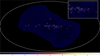 |
Fig. B.1 Example of an IROS solution of a 10 ksec eXTP-WFM (N=3) observation of GX 3+1 for the Sun position on March 15, mapped in an Aitoff projection in Galactic coordinates. The color scale is mapped between 0 and 8 significance. The inset shows a zoomed-in region where the FOVs of two camera pairs overlap. |
All Tables
All Figures
|
Fig. 1 WFM camera shown with the shielding made slightly transparent. In purple, the four SDDs are depicted; the mask is shown on top. |
| In the text | |
|
Fig. 2 A schematic of the WFM configuration foreseen for eXTP as an example. The narrow-field instruments of eXTP are pointed upward, so the WFM pair “0” covers the pointing of those instruments at the center of the FOV. |
| In the text | |
|
Fig. 3 WFM mask. The cyclic difference set is laid down starting from the bottom left, going first from left to right and then bottom to top. |
| In the text | |
|
Fig. 4 Flow diagram of IROS. |
| In the text | |
|
Fig. 5 PSF formation along the “fine” direction. In the top section of the figure, the rays of an off-axis source illuminate the thick mask somewhat sideways and introduce a shadow on one side of the projection of the mask element on the detector (middle blue graph). When cross-correlating with the decoding mask (moving the decoding mask from left to right over the detector; see middle blue graph), this introduces (bottom blue graph) (1) a flat top to the PSF which is off-centered; (2) a lower PSF peak representative of a less sensitive area; and (3) a narrower PSF. The red dots indicate where the discrete cross-correlation would sample the PSF if the sampling is equal to the mask element size. The sampled cross-correlation looks like there is no shadowing, but its integral is actually smaller. |
| In the text | |
|
Fig. 6 Histogram of standard-deviation values of significance images of the GC field solution without Poisson noise for 658 different pointings (i.e., rotating from 0 to 359 deg in steps of 1 deg and for stepping diagonally over the image in 299 steps at one rotation angle). |
| In the text | |
|
Fig. 7 Image of X detector (fine resolution along X) for LMC field for an observation with an exposure time of 10 ks. Unit is photon counts per 0.25 mm × 0.25 mm bin. The color-scale bar of the pixel values is shown at the bottom. The cross is due to the spaces between the four SDD tiles in the detector plane. |
| In the text | |
|
Fig. 8 Part of the sky image of the LMC observation as obtained through IROS, between –28◦ and +40◦ in the local frame along X and –39◦ and +25◦ in Y, zooming in on 40% of the total image (i.e., the fraction of sky pixels), showing the strongest sources in the FOV. The pixel unit is significance. Only sources brighter than 13 mCrab are labeled. The cross-like PSF of a source is not always apparent, because its narrowness is not clear at this image reproduction; it is clearer when zooming in on the pdf version of this paper. |
| In the text | |
|
Fig. 9 Image of X detector for an observation of 10 ks exposure of GC field. The illumination by Sco X-1 is obvious. Unit is photon counts per 0.25 mm × 0.25 mm bin. |
| In the text | |
|
Fig. 10 Part of the sky image of the GC observation as obtained through IROS, between –44◦ and +45◦ in in the local frame along X and –35◦ and +35◦ in Y, zooming in on 70% of the total image (i.e., the fraction of sky pixels) showing the strongest sources in the FOV. The pixel unit is significance. Only sources brighter than 80 mCrab are labeled. The cross-like PSF of a source is not always apparent because its narrowness does not show well at this image reproduction; it is clearer when zooming in the pdf version of this paper. |
| In the text | |
|
Fig. 11 Comparison of sky reconstructions of the GC field between the 2 × 1.5D configuration (right) and the 1 × 2D configuration (left), zooming in on the central quarter of the FOV. |
| In the text | |
|
Fig. 12 Top panel: MLM reconstruction of the spectrum of GRO J1655-40 (data points) and best-fit model spectrum (drawn histogram). For details, see main text. Bottom panel: comparison between data points and model, after setting the normalizations of the two spectral lines to zero. |
| In the text | |
|
Fig. A.1 MLM solution of the central 25 × 25 square degrees of the GC observation, projected on an R.A.-Decl. plane (Eq. 2000.0). Sources are 4U 1820-30 at (R.A., Decl.)=(275.9,-30.4), GX 9+1 at (270.4,-20.5), GX 3+1 at (267.0,-26.5), GX 9+9 at (262.2,-17.0), GX 13+1 at (273.6,-17.2), GX 354-0 at (263.0,-33.8), GX 349+2 at (256.4,-36.4) and partially GRO J1655-40 at (353.5,-39.8). GX 5-1 is missing at (270.3,-25.1) because it is included in ℋ0. The pixel scale is Q (proxy for significance). |
| In the text | |
|
Fig. B.1 Example of an IROS solution of a 10 ksec eXTP-WFM (N=3) observation of GX 3+1 for the Sun position on March 15, mapped in an Aitoff projection in Galactic coordinates. The color scale is mapped between 0 and 8 significance. The inset shows a zoomed-in region where the FOVs of two camera pairs overlap. |
| In the text | |
Current usage metrics show cumulative count of Article Views (full-text article views including HTML views, PDF and ePub downloads, according to the available data) and Abstracts Views on Vision4Press platform.
Data correspond to usage on the plateform after 2015. The current usage metrics is available 48-96 hours after online publication and is updated daily on week days.
Initial download of the metrics may take a while.