| Issue |
A&A
Volume 709, May 2026
|
|
|---|---|---|
| Article Number | A195 | |
| Number of page(s) | 9 | |
| Section | Astrophysical processes | |
| DOI | https://doi.org/10.1051/0004-6361/202659203 | |
| Published online | 13 May 2026 | |
Novae breves from magnetar giant flares: Potential probes of neutron star crusts
1
Department of Astronomy, School of Physics, Peking University, Beijing 100871, China
2
Kavli Institute for Astronomy and Astrophysics, Peking University, Beijing 100871, China
3
Guangxi Key Laboratory for Relativistic Astrophysics, School of Physical Science and Technology, Guangxi University, Nanning 530004, China
4
National Astronomical Observatories, Chinese Academy of Sciences, Beijing 100101, China
★ Corresponding authors: This email address is being protected from spambots. You need JavaScript enabled to view it.
; This email address is being protected from spambots. You need JavaScript enabled to view it.
Received:
29
January
2026
Accepted:
2
April
2026
Abstract
Context. Matter ejected from the magnetar crust during giant flares (GFs) may undergo r-process nucleosynthesis, producing short-lived optical transients termed “novae breves”. Although intrinsically much fainter than kilonovae from compact binary mergers, novae breves may occur within or near the Galaxy, making them promising observational targets.
Aims. We aim to investigate how the neutron star (NS) equation of state (EOS) and the mass of the central magnetar affect the ejecta properties following GFs and the resulting nova brevis emission.
Methods. We employed a semi-analytical ejecta model combined with nuclear reaction network calculations to compute nucleosynthesis yields and multiband light curves for different EOSs and magnetar masses, and we assessed their detectability with current and future facilities.
Results. We find that variations in the EOS and magnetar mass modify the ejecta mass and its density and velocity distributions, among others, leading to observable differences in nova brevis light curves. In particular, both the peak luminosity and the characteristic peak timescale are EOS-dependent. Assuming a fixed Galactic magnetar mass of 1.4 M⊙ and taking the u band as an example, we find that the minimum apparent AB magnitudes range from ∼7 mag (H4 EOS) to ∼8.5 mag (WFF EOS) with peak timescales of ≃102–103 s. A more massive magnetar produces fainter emission with a shorter peak timescale. For a magnetar mass of 1.4 M⊙, novae breves associated with known magnetars may reach peak luminosities of ∼1037–1039 erg s−1, enabling targeted searches, particularly following high-energy GF alerts. Larger ejecta masses yield higher peak luminosities. Moreover, a detection horizon of ≃10 Mpc or beyond is achievable with current and future facilities, allowing searches for novae breves from previously unknown magnetars in the Local Volume.
Conclusions. Although challenging, the detection of such rapidly evolving transients is feasible. Future searches for novae breves can help establish their observational existence and improve our understanding of the NS EOS and crustal properties.
Key words: equation of state / nuclear reactions / nucleosynthesis / abundances / radiation mechanisms: thermal / stars: magnetars
© The Authors 2026
 Open Access article, published by EDP Sciences, under the terms of the Creative Commons Attribution License (https://creativecommons.org/licenses/by/4.0), which permits unrestricted use, distribution, and reproduction in any medium, provided the original work is properly cited.
This article is published in open access under the Subscribe to Open model. This email address is being protected from spambots. You need JavaScript enabled to view it. to support open access publication.
1. Introduction
The Universe hosts hundreds of chemical elements and a vast number of isotopes, yet explaining their cosmic abundance patterns has long been a central problem in nuclear astrophysics. Early theoretical efforts include the seminal Big Bang nucleosynthesis (BBN) framework proposed by Gamow (1948) and Alpher et al. (1948), which aimed to account for the origin of the chemical elements in the early Universe. It is now well established, however, that BBN can produce only the lightest nuclei, primarily hydrogen, helium, and their isotopes (Arcones & Thielemann 2023). Consequently, the synthesis of heavier elements must proceed through astrophysical processes occurring at later cosmic times.
A major breakthrough was achieved by the B2FH theory (Burbidge et al. 1957), which demonstrated that stellar nucleosynthesis, together with mass loss and explosive events such as supernovae (SNe), plays a dominant role in shaping the chemical enrichment of the Universe over cosmic time. Within this framework, the rapid neutron-capture (r) process is particularly crucial for producing elements heavier than iron1. The r process operates under extremely neutron-rich conditions, in which neutron captures proceed on timescales much shorter than those of β decay, driving nuclei toward very high mass numbers before they subsequently decay back toward stability and populate the heavy-element abundance pattern.
However, an increasing number of studies have suggested that achieving sufficiently neutron-rich conditions within stellar interiors or proto-neutron-star (proto-NS) winds following SNe is challenging, typically allowing the synthesis of nuclei only up to mass numbers A ≲ 110 (see e.g., Wanajo et al. 2011; Martinez-Pinedo et al. 2012; Roberts et al. 2012). These limitations have motivated the exploration of alternative astrophysical sites for r-process nucleosynthesis, with compact binary mergers involving NSs, such as NS–NS and NS–black hole (NS–BH) mergers, emerging as leading candidates (Thielemann et al. 2017; Chen et al. 2024). Such mergers can eject substantial amounts of neutron-rich material at high velocities through tidal disruption, shock heating, and post-merger winds, thereby providing favorable conditions for r-process nucleosynthesis. Moreover, compact binary mergers are expected to produce a variety of observable electromagnetic (EM) transients (see e.g., Nakar 2020). Among these, kilonova emissions were initially proposed to arise from the radioactive decay of freshly synthesized r-process nuclei in the merger ejecta, primarily radiating in the ultraviolet (UV), optical, and infrared (IR) bands (Li & Paczynski 1998; Metzger et al. 2010). As such, kilonovae are regarded as a distinctive probe of compact binary mergers (Fernández & Metzger 2016; Barnes et al. 2016; Metzger 2020). Notably, this picture was confirmed by the co-detection of the kilonova AT2017gfo (Andreoni et al. 2017; Arcavi et al. 2017; Chornock et al. 2017; Coulter et al. 2017; Cowperthwaite et al. 2017; Díaz et al. 2017; Drout et al. 2017; Evans et al. 2017; Hu et al. 2017; Kasliwal et al. 2017; Kilpatrick et al. 2017; Lipunov et al. 2017; McCully et al. 2017; Nicholl et al. 2017; Pian et al. 2017; Shappee et al. 2017; Smartt et al. 2017; Soares-Santos et al. 2017; Tanvir et al. 2017; Utsumi et al. 2017; Valenti et al. 2017) in association with the first multi-messenger gravitational-wave event GW170817 from a NS–NS merger (Abbott et al. 2017a,b; Margutti & Chornock 2021).
Despite theoretical and observational success, growing evidence suggests that compact binary mergers alone may not fully account for the total observed abundances of heavy elements in the Galaxy (Côté et al. 2019; Zevin et al. 2019; van de Voort et al. 2020; Thielemann et al. 2020; Tsujimoto 2021), or in extremely metal-poor stars (Qian & Wasserburg 2007; Sneden et al. 2008; Roederer 2013; Ou et al. 2024). These discrepancies indicate that additional r-process sources must contribute to the galactic chemical evolution. Among the proposed candidates, magnetar giant flares (MGFs), originating from magnetars with ultra-strong magnetic fields of 1014–1015 G (Duncan & Thompson 1992), have recently drawn attention as promising sites for ejecting small amounts of neutron-rich material capable of undergoing r-process nucleosynthesis (Cehula et al. 2024; Patel et al. 2025a,b, 2026). Sudden dissipation of ultra-strong magnetic fields above magnetars can trigger a variety of high-energy transient outbursts, among which the most violent are MGFs (Turolla et al. 2015; Popov & Postnov 2007). A generic mechanism for such localized magnetic energy dissipation is magnetic reconnection, which breaks and subsequently reconfigures magnetic field lines. During a MGF, the enhanced external magnetic pressure may drive shocks into the magnetar crust, leading to dissociation of baryonic matter. Before the magnetic field lines fully reconnect, a small fraction of the crust can subsequently be expelled (Demidov & Lyubarsky 2022; Cehula et al. 2024). The resulting ejecta are expected to be neutron-rich, thereby providing favorable conditions for r-process nucleosynthesis and its associated follow-up EM transients.
On the one hand, since the total ejecta mass from a single magnetar is much smaller than that produced in compact binary mergers, the associated optical transients should have lower peak luminosities and shorter characteristic timescales than typical merger-driven kilonovae. Accordingly, such theoretically predicted thermal optical transients following MGFs are referred to as novae breves (Cehula et al. 2024; Patel et al. 2025a,b). On the other hand, because these events can occur within our Galaxy, their proximity may significantly enhance their detectability. Indeed, observational evidence for r-process nucleosynthesis has already been reported in the MGF of SGR 1806−20 (Patel et al. 2025b). If more events are detected in the future, they would not only help improve our understanding of the contribution of different astrophysical sources to the galactic heavy-element inventory, but also provide a unique opportunity to probe magnetar physics, particularly the properties of NS crusts.
Motivated by this, in this work we aim to demonstrate that novae breves associated with MGFs can serve as potential probes of NS crust physics. Specifically, we extend the work of Patel et al. (2025a,b) by investigating how different NS equations of state (EOSs) and magnetar masses affect the properties of the ejecta launched following MGFs and, consequently, the resulting nova brevis emission. We show that variations in the EOS and magnetar mass can alter the ejecta properties, such as the total ejetca masses and its density and velocity distributions, leading to observable signatures in the multiband light curves of novae breves. In particular, both the peak luminosity and the characteristic peak timescale are EOS-dependent. Assuming a fixed Galactic magnetar mass of 1.4 M⊙ and taking the u band as an example, we find that the minimum apparent AB magnitudes (i.e., at peak brightness) range from ∼7 mag for the stiff H4 EOS to ∼8.5 mag for the soft WFF EOS, with peak timescales of ≃102–103 s. A more massive central magnetar generally results in a lower peak luminosity and a shorter peak timescale. Consequently, the detection of such rapidly evolving transients is challenging, but not entirely prohibitive, and a positive detection may offer an indirect avenue for constraining the magnetar crustal properties. We further investigate the detection prospects of these fast and faint novae breves with current and next-generation ground-based and space-borne telescopes. Although not every MGF produces observable nova brevis emission, targeted monitoring offers a promising pathway toward realistic detection from known magnetars, which may generate novae breves with peak bolometric luminosities of ∼1037–1039 erg s−1 for a magnetar mass of 1.4 M⊙. For unknown magnetars, instruments with rapid slewing capabilities and wide fields of view provide a complementary advantage in capturing such short-lived nova brevis transients. A detection horizon of ≃10 Mpc, or even beyond, that is achievable with current and future facilities would encompass the nearest star-forming galaxies within the Local Volume. Overall, our results indicate that future searches for novae breves are feasible. They can not only establish their observational existence, but also improve our understanding of the NS EOS and crustal properties.
The structure of this paper is as follows. In Sect. 2, we briefly present the NS EOSs used in this work, together with the resulting properties of the unbound ejecta and subsequent nucleosynthesis. In Sect. 3, we present the multiband light curves of novae breves for different EOSs and magnetar masses, and discuss the detection prospects of these short-lived transients with current and next-generation facilities. Finally, we summarize in Sect. 4.
2. Baryonic ejecta after MGFs
2.1. NS EOSs
Before investigating the properties of the unbound ejecta and subsequent nucleosynthesis, we first specify the NS EOSs adopted in this work. To explore as broadly as possible the allowed EOS parameter space and the resulting diversity in nova brevis emissions, we consider five representative EOSs: APR, ENG, H4, SLy, and WFF (see e.g., Lattimer & Prakash 2001; Özel & Freire 2016; Lattimer 2021; Gao et al. 2021). These EOSs differ in their particle contents (e.g., the H4 EOS includes hyperons; Lackey et al. 2006), model constructions (e.g., the nonrelativistic Skyrme-Lyon model for the SLy EOS; Chabanat et al. 1998), and underlying theoretical approaches (e.g., variational methods for the APR and WFF EOSs, and Dirac-Brueckner Hartree-Fock calculations for the ENG EOS; Akmal et al. 1998; Engvik et al. 1996; Wiringa et al. 1988). The detailed compositions of these EOSs are summarized in Table 1 of Lattimer & Prakash (2001). The corresponding NS mass–radius (M–R) relations are shown in Fig. 1. For a given EOS and magnetar mass M, the stellar radius R, as well as the internal pressure and density profiles, can be self-consistently determined by solving the Tolman-Oppenheimer-Volkoff equations. For this study, we restricted our analysis to two representative magnetar masses, M = 1.4 M⊙ and M = 2.0 M⊙, and examined the resulting differences in the properties of the corresponding novae breves. Since our study focuses on the outer crust of magnetars, only the region with densities ρ ≲ 4 × 10¹¹ g cm−3 is analyzed further. This choice was well motivated, as only unbound crustal material contributes to the ejecta and, consequently, to the nova brevis emission.
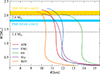 |
Fig. 1. M–R relations for five representative NS EOSs: APR, ENG, H4, SLy, and WFF (Lattimer & Prakash 2001; Özel & Freire 2016; Lattimer 2021). Different colors correspond to different EOSs. For this study, we restricted our analysis to two magnetar masses, M = 1.4 M⊙ and M = 2.0 M⊙, indicated by the horizontal dashed black lines. Observational constraints from PSR J0740+6620 (yellow band; Fonseca et al. 2021) and PSR J0348+0432 (blue band; Saffer et al. 2025) are shown in the figure. |
2.2. Unbound ejecta properties
To obtain the properties of the unbound ejecta for different EOSs and magnetar masses, we followed the model framework introduced by Patel et al. (2025a,b), which is briefly summarized in Appendix A. The resulting unbound ejecta masses are listed in Table 1. As shown in Table 1, for a given magnetar mass, stiffer EOSs generally yield more massive ejecta. This trend naturally arises from the larger stellar radii and weaker gravitational binding associated with stiffer EOSs, which facilitate mass ejection after MGFs. In addition to the total ejecta mass, other EOS-dependent properties, such as the density and velocity distributions, are discussed in Appendix A.
Magnetar radius R and unbound ejecta mass Mej for different EOSs at fixed magnetar masses M.
2.3. Nucleosynthesis for novae breves
Following Patel et al. (2025a), we divided the post-shock unbound ejecta into 30 concentric layers, evolved each layer independently, and tracked their dynamical and thermal evolution together with the associated nucleosynthesis. For a given choice of EOS and magnetar mass, we employed the nuclear reaction network, SkyNet2 (Lippuner & Roberts 2015, 2017), to compute the time-dependent nucleosynthesis and total elemental yields of the ejecta. Based on these nucleosynthesis yields, we subsequently computed the light curves of novae breves, explicitly accounting for the contribution from r-process nuclei. Additional nucleosynthesis results are provided in Appendix B. Details of the light-curve modeling are also described, including several modifications relative to Patel et al. (2025a,b), particularly in the treatment of radioactive heating rates. For the decay energy of heavy r-process nuclei, we adopted the latest data from the Evaluated Nuclear Data File library (ENDF/B-VIII.1; Nobre et al. 2025). Our results show that the total nucleosynthesis yields of the ejecta exhibit non-negligible variations across different EOSs and magnetar masses, especially for heavy elements with A ≳ 140 (see Fig. B.1). These EOS-dependent nucleosynthesis signatures are expected to influence the subsequent nova brevis emission and, consequently, their detectability.
3. Result
3.1. Light curves of novae breves
In Fig. 2 we present the time evolution of the bolometric luminosity for novae breves under different EOSs and magnetar masses. Distinct EOSs lead to noticeable variations in both the peak luminosity and the corresponding peak time. Assuming a fixed magnetar mass of 1.4 M⊙, we find that the peak bolometric luminosity of novae breves can reach ≃1038.5–1039 erg s−1, with peak timescales of ≃102–103 s. A stiffer EOS (e.g., H4) yields a higher peak luminosity and a longer characteristic timescale. This behavior can be naturally understood in terms of the larger ejecta mass associated with stiffer EOSs (see Table 1)3. In addition to the EOS dependence, the magnetar mass also plays an important role in shaping the luminosity evolution of novae breves. As shown in Fig. 2, a more massive magnetar generally results in a lower peak luminosity and a shorter peak timescale. Figure 2 also indicates a degeneracy between the EOS and the magnetar mass; therefore, additional observational constraints on either parameter would help break this degeneracy and better probe the other. For most light curves, we identified a hump-like feature at ≲100 s prior to the luminosity peak. This feature originates from the temporal evolution of the relative recession velocities of the diffusion surface and the photosphere.
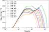 |
Fig. 2. Time evolution of the bolometric luminosity of novae breves for different EOSs and magnetar masses. Different colors correspond to different EOSs. Solid lines show the results for a 1.4 M⊙ magnetar, while dashed lines correspond to the 2.0 M⊙ case. The magnetic field strength is considered to be B ≃ 1015 G. |
In Fig. 3 we show the corresponding u-band light-curve evolution, while results for other bands (e.g., g, r, i, and z) are presented in Fig. B.2. A fiducial Galactic distance of D = 10 kpc was adopted. The u-band light curves exhibit clear EOS-dependent differences in both the minimum apparent AB magnitudes (i.e., at peak brightness), ranging from ∼7 mag for H4 to ∼8.5 mag for WFF, and the peak timescales of ≃102–103 s. The pronounced peaks allowed the peak times to be determined relatively precisely. Similarly to the bolometric case, a more massive magnetar leads to fainter u-band emission and a shorter peak timescale. Together, these results suggest that future detection of nova brevis events could provide valuable information on the crustal properties of magnetars.
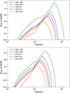 |
Fig. 3. u-band light-curve evolution of novae breves for different EOSs and magnetar masses. Different colors correspond to different EOSs. The upper panel shows the results for a 1.4 M⊙ magnetar, while the lower panel corresponds to the 2.0 M⊙ case. A fiducial Galactic distance of D = 10 kpc was adopted, and the magnetic field strength is considered to be B ≃ 1015 G. |
3.2. Detection prospects
As shown in Fig. 2 and Fig. 3, the peak optical luminosity of novae breves is expected to be comparable to that of typical Galactic novae, but with peak timescales of several tens of minutes at most. The detection of such rapidly evolving transients is therefore challenging, although not entirely prohibitive.
For known magnetars, while the occurrence time of potential nova brevis events cannot be predicted in advance, highly sensitive ground-based and space-borne facilities – such as the Large Synoptic Survey Telescope (LSST, now the Vera C. Rubin Observatory; Abell et al. 2009; Ivezić et al. 2019) – may lead to their discovery. For previously unknown magnetars within or near our Galaxy, instruments with short slewing times or large fields of view can substantially enhance the detection probability. For example, the UltraViolet/Optical Telescope (UVOT) aboard the Neil Gehrels Swift Observatory can switch to a target within ≲100 s following a high-energy trigger (Roming et al. 2005), for example, from MGFs. Similarly, wide-field survey facilities such as the Wide Field Survey Telescope (WFST; Wang et al. 2023) and the Chinese Space Station Telescope (CSST; Wei et al. 2026) also have the potential to detect novae breves associated with MGFs.
To quantitatively assess the detection prospects with current and future facilities, we selected magnetars with measured distances and magnetic field strengths from the McGill Magnetar Catalog4 (Olausen & Kaspi 2014). In Table 2, we list the peak bolometric luminosities of the corresponding nova brevis events for different EOSs. Magnetars yielding a total ejecta mass of Mej < 10−9 M⊙ have been excluded, as such small ejecta masses are unlikely to support significant nucleosynthesis during a nova brevis event. Assuming a fixed magnetar mass of 1.4 M⊙, these systems are expected to produce novae breves with peak bolometric luminosities of ∼1037–1039 erg s−1, comparable to that of typical Galactic novae5.
Selected known magnetars and their properties.
In Fig. 4, we show the minimum u-band apparent AB magnitudes (at peak brightness) and the corresponding peak times for each selected magnetar. Among the EOSs, the stiffest (H4) and softest (WFF) are indicated by red and blue labels, respectively. We overlaid the limiting detection magnitudes as functions of exposure time for LSST6, UVOT7, WFST (Lei et al. 2023), and CSST (Wei et al. 2026), using different line styles. As illustrated, if nova brevis events indeed occur in these magnetar systems, such short-lived transients are potentially detectable with these facilities, particularly when observations are triggered by high-energy alerts from MGFs.
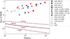 |
Fig. 4. Minimum u-band apparent AB magnitudes (i.e., at peak brightness) and the corresponding peak times for selected magnetars in Table 2. A fixed magnetar mass of 1.4 M⊙ was adopted. Different symbols represent different magnetars. Among the EOSs considered in this work, the stiffest (H4) and softest (WFF) are indicated by red and blue labels, respectively. The limiting magnitudes as functions of exposure time for different telescopes have been overplotted for UVOT, WFST, LSST, and CSST. The region above each line corresponds to the detectable parameter space. |
Furthermore, assuming a representative peak optical luminosity of 1038 erg s−1 for novae breves, we show the corresponding detection horizons for different facilities in Fig. 5. A horizon of ≃10 Mpc, or even beyond, appears achievable with current and next-generation ground-based and space-borne telescopes. This implies that nearby star-forming galaxies within the Local Volume can be encompassed in systematic searches for nova brevis events.
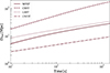 |
Fig. 5. Detection horizons of novae breves for different facilities, assuming a representative peak optical luminosity of 1038 erg s−1. Different line styles denote different telescopes. |
4. Conclusion
Building on previous studies of novae breves powered by the radioactive decay of heavy r-process nuclei in MGF ejecta, we have investigated how different NS EOSs and central magnetar masses affect the properties of the ejecta launched following MGFs and the resulting nova brevis emission. Our calculations show that variations in the EOS and magnetar mass can alter the total ejecta mass, as well as its density and velocity distributions, among others, leading to observable differences in the nova brevis light curves. In particular, both the peak luminosity and the characteristic peak timescale are EOS-dependent. Assuming a fixed Galactic magnetar mass of 1.4 M⊙ and taking the u band as an example, we find that the minimum apparent AB magnitudes (i.e., at peak brightness) range from ∼7 mag for the H4 EOS to ∼8.5 mag for the WFF EOS, with peak timescales of ≃102–103 s. In addition, a more massive central magnetar generally results in a lower peak luminosity and a shorter peak timescale, indicating a degeneracy between the magnetar mass and the EOS. The detection of such rapidly evolving transients is challenging, but not entirely prohibitive. Their detection may offer an indirect avenue for constraining the magnetar crustal properties.
We further explore the detection prospects of these fast and faint novae breves with current and next-generation telescopes. Although not every MGF produces an observable nova brevis emission, targeted monitoring provides a promising pathway toward realistic detection from known magnetars, which may generate novae breves with peak bolometric luminosities of ∼1037–1039 erg s−1, comparable to that of typical Galactic novae. For unknown magnetars, instruments with rapid slewing capabilities and wide fields of view have a complementary advantage when capturing such short-lived nova brevis transients. A detection horizon of ≃10 Mpc, or even beyond, that is achievable with current and future facilities would encompass the nearest star-forming galaxies within the Local Volume.
It is important to note that we adopted the mass ejection model proposed by Cehula et al. (2024), and our results therefore apply specifically within the framework of that study. The exact mass ejection mechanism, however, remains uncertain. For example, Bransgrove et al. (2025) performed two-dimensional magnetohydrodynamic simulations of a markedly different scenario in which baryon ejection is driven by the eruption of baryon-loaded magnetic loops from the NS interior. These differences highlight the need for further investigation of the mass ejection process. Overall, our results indicate that future searches for novae breves are feasible. Continued theoretical and observational efforts will be essential to confirm such transients and deepen our understanding of NS physics and the origin of heavy elements.
Acknowledgments
We thank the anonymous referee for helpful comments. This work is supported by the Beijing Natural Science Foundation (QY25099, 1242018), the National Natural Science Foundation of China (12573042, 12403043, and 12473038), the National SKA Program of China (2020SKA0120300), the Max Planck Partner Group Program funded by the Max Planck Society, and the High-Performance Computing Platform of Peking University.
References
- Abbott, B. P., Abbott, R., Abbott, T. D., et al. 2017a, Phys. Rev. Lett., 119, 161101 [Google Scholar]
- Abbott, B. P., Abbott, R., Abbott, T. D., et al. 2017b, ApJ, 848, L12 [Google Scholar]
- Abell, P. A., Allison, J., Anderson, S. F., et al. 2009, ArXiv e-prints [arXiv:0912.0201] [Google Scholar]
- Akmal, A., Pandharipande, V. R., & Ravenhall, D. G. 1998, Phys. Rev. C, 58, 1804 [Google Scholar]
- Alpher, R. A., Bethe, H., & Gamow, G. 1948, Phys. Rev., 73, 803 [CrossRef] [Google Scholar]
- Andreoni, I., Ackley, K., Cooke, J., et al. 2017, PASA, 34, e069 [NASA ADS] [CrossRef] [Google Scholar]
- Arcavi, I., Hosseinzadeh, G., Howell, D. A., et al. 2017, Nature, 551, 64 [NASA ADS] [CrossRef] [Google Scholar]
- Arcones, A., & Thielemann, F.-K. 2023, A&ARv., 31, 1 [Google Scholar]
- Barnes, J., Kasen, D., Wu, M.-R., & Martínez-Pinedo, G. 2016, ApJ, 829, 110 [NASA ADS] [CrossRef] [Google Scholar]
- Bransgrove, A., Beloborodov, A. M., & Levin, Y. 2025, ArXiv e-prints [arXiv:2508.13419] [Google Scholar]
- Burbidge, M. E., Burbidge, G. R., Fowler, W. A., & Hoyle, F. 1957, Rev. Mod. Phys., 29, 547 [Google Scholar]
- Cehula, J., Thompson, T. A., & Metzger, B. D. 2024, MNRAS, 528, 5323 [Google Scholar]
- Chabanat, E., Bonche, P., Haensel, P., Meyer, J., & Schaeffer, R. 1998, Nucl. Phys. A, 635, 231 [NASA ADS] [CrossRef] [Google Scholar]
- Chen, M.-H., & Liang, E.-W. 2023, MNRAS, 527, 5540 [Google Scholar]
- Chen, M.-H., Li, L.-X., Chen, Q.-H., Hu, R.-C., & Liang, E.-W. 2024, MNRAS, 529, 1154 [Google Scholar]
- Chornock, R., Berger, E., Kasen, D., et al. 2017, ApJ, 848, L19 [NASA ADS] [CrossRef] [Google Scholar]
- Côté, B., Eichler, M., Arcones, A., et al. 2019, ApJ, 875, 106 [Google Scholar]
- Coulter, D. A., Foley, R. J., Kilpatrick, C. D., et al. 2017, Science, 358, 1556 [NASA ADS] [CrossRef] [Google Scholar]
- Cowperthwaite, P. S., Berger, E., Villar, V. A., et al. 2017, ApJ, 848, L17 [CrossRef] [Google Scholar]
- Demidov, I., & Lyubarsky, Y. 2022, MNRAS, 518, 810 [Google Scholar]
- Díaz, M. C., Macri, L. M., Lambas, D. G., et al. 2017, ApJ, 848, L29 [Google Scholar]
- Drout, M. R., Piro, A. L., Shappee, B. J., et al. 2017, Science, 358, 1570 [NASA ADS] [CrossRef] [Google Scholar]
- Duncan, R. C., & Thompson, C. 1992, ApJ, 392, L9 [Google Scholar]
- Engvik, L., Bao, G., Hjorth-Jensen, M., Osnes, E., & Ostgaard, E. 1996, ApJ, 469, 794 [Google Scholar]
- Evans, P. A., Cenko, S. B., Kennea, J. A., et al. 2017, Science, 358, 1565 [NASA ADS] [CrossRef] [Google Scholar]
- Fernández, R., & Metzger, B. D. 2016, Ann. Rev. Nucl. Part. Sci., 66, 23 [CrossRef] [Google Scholar]
- Fonseca, E., Cromartie, H. T., Pennucci, T. T., et al. 2021, ApJ, 915, L12 [NASA ADS] [CrossRef] [Google Scholar]
- Gamow, G. 1948, Nature, 162, 680 [Google Scholar]
- Gao, Y., Lai, X.-Y., Shao, L., & Xu, R.-X. 2021, MNRAS, 509, 2758 [Google Scholar]
- Hu, L., Jiang, R., Chen, X., et al. 2017, Sci. Bull., 62, 1433 [Google Scholar]
- Ivezić, Ž., Kahn, S. M., Tyson, J. A., et al. 2019, ApJ, 873, 111 [Google Scholar]
- Kasen, D., & Barnes, J. 2019, ApJ, 876, 128 [Google Scholar]
- Kasliwal, M. M., Nakar, E., Singer, L. P., et al. 2017, Science, 358, 1559 [NASA ADS] [CrossRef] [Google Scholar]
- Kilpatrick, C. D., Foley, R. J., Kasen, D., et al. 2017, Science, 358, 1583 [NASA ADS] [CrossRef] [Google Scholar]
- Lackey, B. D., Nayyar, M., & Owen, B. J. 2006, Phys. Rev. D, 73, 024021 [Google Scholar]
- Lattimer, J. M. 2021, Ann. Rev. Nucl. Part. Sci., 71, 433 [NASA ADS] [CrossRef] [Google Scholar]
- Lattimer, J. M., & Prakash, M. 2001, ApJ, 550, 426 [NASA ADS] [CrossRef] [Google Scholar]
- Lei, L., Zhu, Q.-F., Kong, X., et al. 2023, Res. Astron. Astrophys., 23, 035013 [Google Scholar]
- Li, L.-X., & Paczynski, B. 1998, ApJ, 507, L59 [NASA ADS] [CrossRef] [Google Scholar]
- Lippuner, J., & Roberts, L. F. 2015, ApJ, 815, 82 [CrossRef] [Google Scholar]
- Lippuner, J., & Roberts, L. F. 2017, ApJS, 233, 18 [NASA ADS] [CrossRef] [Google Scholar]
- Lipunov, V. M., Gorbovskoy, E., Kornilov, V. G., et al. 2017, ApJ, 850, L1 [NASA ADS] [CrossRef] [Google Scholar]
- Margutti, R., & Chornock, R. 2021, ARA&A, 59, 155 [NASA ADS] [CrossRef] [Google Scholar]
- Martinez-Pinedo, G., Fischer, T., Lohs, A., & Huther, L. 2012, Phys. Rev. Lett., 109, 251104 [Google Scholar]
- McCully, C., Hiramatsu, D., Howell, D. A., et al. 2017, ApJ, 848, L32 [NASA ADS] [CrossRef] [Google Scholar]
- Metzger, B. D. 2020, Liv. Rev. Relativ., 23, 1 [NASA ADS] [CrossRef] [Google Scholar]
- Metzger, B. D., Martinez-Pinedo, G., Darbha, S., et al. 2010, MNRAS, 406, 2650 [NASA ADS] [CrossRef] [Google Scholar]
- Nakar, E. 2020, Phys. Rept., 886, 1 [Google Scholar]
- Nicholl, M., Berger, E., Kasen, D., et al. 2017, ApJ, 848, L18 [NASA ADS] [CrossRef] [Google Scholar]
- Nobre, G. P. A., Capote, R., Pigni, M. T., et al. 2025, ArXiv e-prints [arXiv:2511.03564] [Google Scholar]
- Olausen, S. A., & Kaspi, V. M. 2014, ApJS, 212, 6 [Google Scholar]
- Ou, X., Ji, A. P., Frebel, A., Naidu, R. P., & Limberg, G. 2024, ApJ, 974, 232 [NASA ADS] [CrossRef] [Google Scholar]
- Özel, F., & Freire, P. 2016, Ann. Rev. Astron. Astrophys., 54, 401 [CrossRef] [Google Scholar]
- Patel, A., Metzger, B. D., Cehula, J., et al. 2025a, ApJ, 984, L29 [Google Scholar]
- Patel, A., Metzger, B. D., Goldberg, J. A., et al. 2025b, ApJ, 985, 234 [Google Scholar]
- Patel, A., Diesing, R., & Metzger, B. 2026, ApJ, submitted [arXiv:2601.00953] [Google Scholar]
- Pian, E., D’Avanzo, P., Benetti, S., et al. 2017, Nature, 551, 67 [Google Scholar]
- Popov, S. B., & Postnov, K. A. 2007, ArXiv e-prints [arXiv:0710.2006] [Google Scholar]
- Qian, Y. Z., & Wasserburg, G. J. 2007, Phys. Rept., 442, 237 [Google Scholar]
- Qiumu, W.-Z., Chen, M.-H., Chen, Q.-H., & Liang, E.-W. 2025, Res. Astron. Astrophys., 25, 035005 [Google Scholar]
- Roberts, L. F., Reddy, S., & Shen, G. 2012, Phys. Rev. C, 86, 065803 [Google Scholar]
- Roederer, I. U. 2013, AJ, 145, 26 [CrossRef] [Google Scholar]
- Roming, P. W. A., Kennedy, T. E., Mason, K. O., et al. 2005, Space Sci. Rev., 120, 95 [Google Scholar]
- Saffer, A., Fonseca, E., Ransom, S., et al. 2025, ApJ, 983, L20 [Google Scholar]
- Shappee, B. J., Simon, J. D., Drout, M. R., et al. 2017, Science, 358, 1574 [NASA ADS] [CrossRef] [Google Scholar]
- Smartt, S. J., Chen, T.-W., Jerkstrand, A., et al. 2017, Nature, 551, 75 [Google Scholar]
- Sneden, C., Cowan, J. J., & Gallino, R. 2008, ARA&A, 46, 241 [Google Scholar]
- Soares-Santos, M., Holz, D. E., Annis, J., et al. 2017, ApJ, 848, L16 [CrossRef] [Google Scholar]
- Tanvir, N. R., Levan, A. J., González-Fernández, C., et al. 2017, ApJ, 848, L27 [CrossRef] [Google Scholar]
- Thielemann, F. K., Eichler, M., Panov, I. V., & Wehmeyer, B. 2017, Ann. Rev. Nucl. Part. Sci., 67, 253 [Google Scholar]
- Thielemann, F.-K., Wehmeyer, B., & Wu, M.-R. 2020, J. Phys. Conf. Ser., 1668, 012044 [Google Scholar]
- Tsujimoto, T. 2021, ApJ, 920, L32 [Google Scholar]
- Turolla, R., Zane, S., & Watts, A. 2015, Rept. Prog. Phys., 78, 116901 [Google Scholar]
- Utsumi, Y., Tanaka, M., Tominaga, N., et al. 2017, PASJ, 69, 101 [CrossRef] [Google Scholar]
- Valenti, S., Sand, D. J., Yang, S., et al. 2017, ApJ, 848, L24 [CrossRef] [Google Scholar]
- van de Voort, F., Pakmor, R., Grand, R. J. J., et al. 2020, MNRAS, 494, 4867 [NASA ADS] [CrossRef] [Google Scholar]
- Wanajo, S., Janka, H.-T., & Mueller, B. 2011, ApJ, 726, L15 [NASA ADS] [CrossRef] [Google Scholar]
- Wang, T., Liu, G., Cai, Z., et al. 2023, Sci. China Phys. Mech. Astron., 66, 109512 [NASA ADS] [CrossRef] [Google Scholar]
- Wei, C.-L., Li, G.-L., Fang, Y.-D., et al. 2026, Res. Astron. Astrophys., 26, 024001 [Google Scholar]
- Wiringa, R. B., Fiks, V., & Fabrocini, A. 1988, Phys. Rev. C, 38, 1010 [Google Scholar]
- Zevin, M., Kremer, K., Siegel, D. M., et al. 2019, ApJ, 886, 4 [NASA ADS] [CrossRef] [Google Scholar]
We refer readers to Arcones & Thielemann (2023) for a more comprehensive review.
In some NS–NS merger scenarios, a stiffer EOS tends to produce less ejecta and power dimmer kilonova emission (Qiumu et al. 2025), which contrasts with the MGF scenario considered here. This difference arises because stiffer EOSs lead to earlier mergers at larger orbital separations and lower orbital velocities, as well as higher sound speeds that make shock heating of NS matter less efficient.
Patel et al. (2025b) reported that SGR 1806−20 may eject 10−6 M⊙ of material, with a peak luminosity of ∼1040 erg s−1 inferred from a delayed MeV signal. Our results are consistent with these findings, since the ejecta mass obtained in our model is smaller, naturally leading to a lower peak luminosity.
Appendix A: Overview of the unbound ejecta model
For a given EOS and magnetar mass M, we compute the stellar radius R as well as the internal pressure and density profiles, P(r) and ρ(r), respectively (see e.g., Lattimer & Prakash 2001; Özel & Freire 2016; Lattimer 2021; Gao et al. 2021). Within the magnetar crust, the condition of hydrostatic equilibrium gives
 (A.1)
(A.1)
where G is the gravitational constant, and g(r) is the local gravitational acceleration, which is approximated as constant across the relatively thin crustal layer. Under this approximation, the mass of crustal material enclosed above a given radius r is
 (A.2)
(A.2)
Therefore, specifying the inner boundary of the unbound region–equivalently, the critical pressure or density at that boundary–uniquely determines the total mass of the unbound ejecta.
Following Patel et al. (2025a,b), we consider that the energy released during a MGF not only generates a pair-photon fireball above the magnetar surface, but also drives a strong radiation-dominated shock into the magnetar crust. For a typical magnetar, the magnetic field strength in the magnetosphere is B ≃ 1014–1015 G. The external pressure exerted on the crust during MGFs can therefore be approximated as Pext ≳ B2/8π. For a shocked crustal layer to ultimately escape from the star, Patel et al. (2025a,b) derived the maximum crustal density, corresponding to the innermost unbound layer, as
 (A.3)
(A.3)
Combining Eq. (A.2) and Eq. (A.3), together with the pressure–density relation P(ρ), the total unbound ejecta mass Mej can be calculated for different EOSs and magnetar masses. The resulting values are listed in Table 1.
Assuming homologous expansion, Rej ∝ vt, the volume element of each ejecta layer scales as  . Motivated by hydrodynamical simulations (Cehula et al. 2024), the unbound ejecta are assumed to follow a distribution of asymptotic velocities given by
 (A.4)
(A.4)
where we adopt the Lagrangian mass coordinate m ≡ Mcr(> r). In this work we take α ≃ 4 (Patel et al. 2025a,b). After normalization, the velocity profile of the ejecta can be written as
 (A.5)
(A.5)
where vi denotes the velocity of the innermost ejecta layer. We adopt vi ≃ 0.2c with the speed of light c, consistent with Cehula et al. (2024) and Patel et al. (2025a,b). The corresponding density profile can then be estimated as ρ ≃ dm/dV ∝ v−6. After normalization, this yields
 (A.6)
(A.6)
As discussed by Patel et al. (2025a,b), Eq. (A.6) applies during the late-time three-dimensional expansion phase. At earlier times, the ejecta evolution is better approximated as a planar one-dimensional expansion with constant velocity. Accordingly, the Lagrangian density evolution can be written as
 (A.7)
(A.7)
where t0 denotes the start time of the nucleosynthesis (see Appendix B), and tD ≡ 2R/v is the time at which each ejecta layer has expanded by a distance comparable to the magnetar diameter. Using Eq. (A.6), the density at tD is  . The initial density is then ρ0 = ρDtD/t0.
Moreover, the temperature of each ejecta layer at the start time, T0 = T(t0), is determined by the initial density ρ0 and the specific entropy. Following Patel et al. (2025a,b), we adopt the immediate post-shock density ρsh ≈ 7ρcr and the specific internal energy esh ≈ 3Pext/ρsh, as implied by the Rankine–Hugoniot jump conditions (see e.g., Eq. (3) and Eq. (4) in Patel et al. 2025b). These quantities are used to infer the specific entropy, and hence the initial temperature distribution of the unbound ejecta, which serves as input for the subsequent nucleosynthesis calculations performed with SkyNet (Lippuner & Roberts 2015, 2017). Readers interested in more technical details are referred to Appendix A of Patel et al. (2025b).
Appendix B: Nucleosynthesis and light-curve calculations
For each adopted NS EOS and magnetar mass, we perform nucleosynthesis calculations using the SkyNet reaction network (Lippuner & Roberts 2015, 2017), from which we obtain the time evolution of nuclear abundances and the corresponding total elemental yields of the ejecta. The resulting total abundance patterns are compared in Fig. B.1
 |
Fig. B.1. Total nucleosynthesis yields of the ejecta computed with SkyNet for different EOSs and magnetar masses. The magnetic field strength is considered to be B ≃ 1015 G. |
Following Patel et al. (2025a,b), the bolometric luminosity of novae breves is primarily determined by the radioactive energy deposited within the optically thick ejecta. Using the Lagrangian mass coordinate m ≤ Mej, where m = 0 corresponds to the outermost layer of the ejecta, the time-dependent luminosity can be expressed as
 (B.1)
(B.1)
where Mph and Mdiff are the mass coordinates of the photosphere and the diffusion surface, respectively, and  denotes the specific heating rate. The photosphere is defined as the layer at which the optical depth satisfies τ ≃ 2/3, while the diffusion surface corresponds to τ = c/v. Above the diffusion surface, the photon diffusion timescale becomes shorter than the dynamical expansion timescale, allowing photons to escape efficiently without significant adiabatic losses. As a result, the region bounded by the diffusion surface and the photosphere provides the dominant contribution to the bolometric luminosity. Notably, the optical depth is computed as τ = ∫Rej∞κρ dRej, where the opacity evolves with time according to (Patel et al. 2025b),
 (B.2)
(B.2)
where Xi(t) represents the mass fraction of the i-th species. The adopted component opacities are κp ≈ 0.38 cm2 g−1 for protons, κα ≈ 0.2 cm2 g−1 for alpha particles, κseed ≈ 0.5 cm2 g−1 for light seed nuclei, κ2nd ≈ 3 cm2 g−1 for second-peak r-process nuclei, and κ3rd ≈ 20 cm2 g−1 for third-peak r-process nuclei.
The total specific heating rate  is computed by summing the contributions from α, β, and γ decays occurring in the unbound ejecta, i.e.,
 (B.3)
(B.3)
where fn(t) denotes the thermalization efficiency of each decay channel. The specific radioactive heating rate  is obtained by summing over all unstable nuclides in the ejecta,
 (B.4)
(B.4)
where NA is Avogadro’s number, λi = ln2/T1/2 , i is the decay rate of the i-th nuclide with half-life T1/2 , i, Yi(t) is its abundance, and En is the energy released per decay in channel n. For heavy r-process nuclei, the decay energies are taken from the Evaluated Nuclear Data File library (ENDF/B-VIII.1; Nobre et al. 2025).
For the thermalization efficiency fn(t), we adopt the analytic prescriptions of Kasen & Barnes (2019). For β decay, we use
 (B.5)
(B.5)
where the characteristic thermalization timescale tβ is given by
 (B.6)
(B.6)
with Mej the total ejecta mass and vej the characteristic ejecta velocity. ζ is a dimensionless constant, for which we adopt ζ ≃ 1 (Chen & Liang 2023). For α decay, the thermalization efficiency is approximated as
 (B.7)
(B.7)
where the corresponding thermalization timescale is tα ≃ 3tβ. For γ emission, we adopt
 (B.8)
(B.8)
with the thermalization timescale,
 (B.9)
(B.9)
where we adopt a γ-ray opacity of κγ ≃ 0.02 cm2 g−1.
The monochromatic flux density at an observing frequency ν is given by
![Mathematical equation: $$ \begin{aligned} F_{\nu }=\frac{2\pi h{\nu }^3}{c^2}\,\left[{\mathrm{exp} (\dfrac{\,h\nu }{kT_{\mathrm{ph} }})-1}\right]^{-1}\,\frac{R_{\mathrm{ph} }^2}{D^2}\,, \end{aligned} $$](/articles/aa/full_html/2026/05/aa59203-26/aa59203-26-eq22.gif) (B.10)
(B.10)
where h is the Planck constant, Rph is the photospheric radius, D is the luminosity distance, and Tph denotes the photospheric temperature. Using Eq. (B.1), the photospheric temperature is estimated as
 (B.11)
where σ is the Steffan–Boltzmann constant. The corresponding AB magnitude is then computed as mAB = −2.5 log10(Fν / 3631 Jy).
In addition to the u-band light-curve evolution of novae breves for different EOSs and magnetar masses shown in Fig. 3, we also present their corresponding light curves in other optical bands (g, r, i, z) in Fig. B.2.
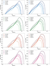 |
Fig. B.2. Similar to Fig. 3, but for (from top down) g, r, i, and z bands. Different colors correspond to different EOSs. The left panels show the results for a 1.4 M⊙ magnetar, while the right panels correspond to the 2.0 M⊙ case. A fiducial Galactic distance of D = 10 kpc is used. |
All Tables
Magnetar radius R and unbound ejecta mass Mej for different EOSs at fixed magnetar masses M.
All Figures
|
Fig. 1. M–R relations for five representative NS EOSs: APR, ENG, H4, SLy, and WFF (Lattimer & Prakash 2001; Özel & Freire 2016; Lattimer 2021). Different colors correspond to different EOSs. For this study, we restricted our analysis to two magnetar masses, M = 1.4 M⊙ and M = 2.0 M⊙, indicated by the horizontal dashed black lines. Observational constraints from PSR J0740+6620 (yellow band; Fonseca et al. 2021) and PSR J0348+0432 (blue band; Saffer et al. 2025) are shown in the figure. |
| In the text | |
|
Fig. 2. Time evolution of the bolometric luminosity of novae breves for different EOSs and magnetar masses. Different colors correspond to different EOSs. Solid lines show the results for a 1.4 M⊙ magnetar, while dashed lines correspond to the 2.0 M⊙ case. The magnetic field strength is considered to be B ≃ 1015 G. |
| In the text | |
|
Fig. 3. u-band light-curve evolution of novae breves for different EOSs and magnetar masses. Different colors correspond to different EOSs. The upper panel shows the results for a 1.4 M⊙ magnetar, while the lower panel corresponds to the 2.0 M⊙ case. A fiducial Galactic distance of D = 10 kpc was adopted, and the magnetic field strength is considered to be B ≃ 1015 G. |
| In the text | |
|
Fig. 4. Minimum u-band apparent AB magnitudes (i.e., at peak brightness) and the corresponding peak times for selected magnetars in Table 2. A fixed magnetar mass of 1.4 M⊙ was adopted. Different symbols represent different magnetars. Among the EOSs considered in this work, the stiffest (H4) and softest (WFF) are indicated by red and blue labels, respectively. The limiting magnitudes as functions of exposure time for different telescopes have been overplotted for UVOT, WFST, LSST, and CSST. The region above each line corresponds to the detectable parameter space. |
| In the text | |
|
Fig. 5. Detection horizons of novae breves for different facilities, assuming a representative peak optical luminosity of 1038 erg s−1. Different line styles denote different telescopes. |
| In the text | |
|
Fig. B.1. Total nucleosynthesis yields of the ejecta computed with SkyNet for different EOSs and magnetar masses. The magnetic field strength is considered to be B ≃ 1015 G. |
| In the text | |
|
Fig. B.2. Similar to Fig. 3, but for (from top down) g, r, i, and z bands. Different colors correspond to different EOSs. The left panels show the results for a 1.4 M⊙ magnetar, while the right panels correspond to the 2.0 M⊙ case. A fiducial Galactic distance of D = 10 kpc is used. |
| In the text | |
Current usage metrics show cumulative count of Article Views (full-text article views including HTML views, PDF and ePub downloads, according to the available data) and Abstracts Views on Vision4Press platform.
Data correspond to usage on the plateform after 2015. The current usage metrics is available 48-96 hours after online publication and is updated daily on week days.
Initial download of the metrics may take a while.