


| Issue |
A&A
Volume 711, July 2026
|
|
|---|---|---|
| Article Number | A248 | |
| Number of page(s) | 14 | |
| Section | Astrophysical processes | |
| DOI | https://doi.org/10.1051/0004-6361/202659110 | |
| Published online | 21 July 2026 | |
Interstellar medium modulation of nonlinear kinetic Alfvén morphology in structured Galactic environments
1
School of Computing and Artificial Intelligence, Southwest Jiaotong University, Chengdu 610031, PR China
2
School of Physical Science and Technology, Southwest Jiaotong University, Chengdu 610031, PR China
3
Department of Physics, Guru Nanak Dev University, Amritsar 143005, India
★ Corresponding author: This email address is being protected from spambots. You need JavaScript enabled to view it.
Received:
23
January
2026
Accepted:
9
June
2026
Abstract
Context. The ionized interstellar medium (ISM) is a structured, magnetized plasma in which large-scale variations in density, magnetic field strength, temperature, and plasma beta can regulate the local existence and morphology of nonlinear waves such as kinetic Alfvén (KA) solitons.
Aims. The aim of this work is to determine how the plasma conditions of a structured Galactic ISM control where nonlinear KA solitons can exist and how their amplitude and width change across different Galactic environments.
Methods. We constructed a multicomponent Galactic ISM model for the diffuse warm ionized medium together with embedded H II regions, stellar-wind bubbles (SWBs), and supernova remnants (SNRs). The reductive perturbation method was then used to derive the Korteweg–de Vries (KdV) equation and its local coefficients, allowing the admissibility, amplitude, and width of KA solitons to be evaluated under realistic plasma conditions, including suprathermality, plasma beta, temperature, and density gradients.
Results. We identify distinct exclusion zones for KA solitons in high-β H II regions and hot SWB and SNR interiors, as well as ultra-low-β regions near central pulsar wind nebulae. The compressed shells of SWBs and SNRs emerge as preferential zones where the KA ordering can remain valid. Within the present leading-order KdV treatment, the soliton width shows the strongest environmental sensitivity, broadening significantly near admissibility boundaries, whereas the amplitude varies more weakly.
Conclusions. This work provides Galactic maps of where nonlinear KA solitons are locally admissible in a structured ISM, together with the corresponding changes in their width and amplitude. These results establish a physically grounded framework for future observational tests for small-scale ISM structures associated with KA solitons.
Key words: ISM: bubbles / HII regions / ISM: supernova remnants
© The Authors 2026
 Open Access article, published by EDP Sciences, under the terms of the Creative Commons Attribution License (https://creativecommons.org/licenses/by/4.0), which permits unrestricted use, distribution, and reproduction in any medium, provided the original work is properly cited.
This article is published in open access under the Subscribe to Open model. This email address is being protected from spambots. You need JavaScript enabled to view it. to support open access publication.
1. Introduction
The ionized interstellar medium (ISM) is now firmly established as a turbulent (Ferrière 2019), magnetized plasma whose electron density fluctuations span more than ten orders of magnitude in scale. Radio scintillation and scattering measurements reveal a nearly Kolmogorov spectrum extending from ∼106 to at least ∼1013 m, forming the “big power law in the sky” (Armstrong et al. 1995). Using Hα observations, Chepurnov & Lazarian (2010) demonstrated that this turbulent cascade continues to scales approaching several parsecs throughout the warm ionized medium (WIM). Pulsar scintillation studies further show that the cascade reaches down to an inner scale of 105–106 m, comparable to the proton gyroradius (Spangler & Gwinn 1990; Rickett et al. 2009; Ocker et al. 2021), implying that interstellar turbulence routinely extends to ion-kinetic scales where the magnetohydrodynamic approximation breaks down. Interstellar scintillation also reveals intermittent, localized electron density structures with non-Gaussian statistics (Boldyrev & Gwinn 2003, 2005; Terry & Smith 2007), suggesting the presence of steepened, coherent plasma fluctuations that resemble nonlinear dispersive structures.
At sub-ion scales, kinetic theory predicts that the Alfvénic cascade transitions naturally into kinetic Alfvén waves (KAWs), which mediate energy transfer to small scales and ultimately to particle heating and acceleration. Gyrokinetic theory (Schekochihin et al. 2009) and solar-wind simulations (Howes et al. 2008a,b; Zhao et al. 2016) demonstrate that KAWs dominate between ion and electron gyroscales, with dissipation primarily via Landau damping, and recent work shows that KAW intermittency can lead to efficient electron heating (Zhou et al. 2023). Observations indicate that plasma beta in the WIM spans a broad range (Ferrière 2001). While some regions approach β ∼ 1, substantial regions of the diffuse ionized medium exhibit β < 1, falling within the regime me/mi ≪ β ≪ 1 (with me and mi being the electron and ion mass, respectively), where KAWs and their nonlinear extensions can exist. Since the WIM is a magnetized, weakly collisional plasma with a cascade extending to ion-kinetic scales, KAW turbulence is a natural candidate for shaping small-scale structure and dissipation in the ISM.
Although the linear and turbulent properties of KAWs are well understood, the formation of nonlinear coherent KAW structures with steepened fronts, localized wave packets, and solitary pulses has received comparatively little attention in an astrophysical ISM context. Spacecraft measurements in the terrestrial magnetosphere reveal localized, dispersive Alfvén (e.g., KAWs) wave packets carrying substantial Poynting flux into the auroral region (e.g., Chaston et al. 2003, 2008), and the review by Stasiewicz et al. (2000) summarizes extensive observations and the theory of small-scale Alfvénic structures, including density cavities, vortices, and steepened fronts. Analytical and observational studies further show that finite-amplitude KAWs can undergo nonlinear steepening and form localized, coherent structures under suitable plasma conditions (Stasiewicz et al. 2000; Singh et al. 2019). However, these works focus on localized, relatively homogeneous space or planetary plasma environments and do not address how coherent KAW structures develop within the highly structured Galactic ISM. Intermittent small-scale density and magnetic structures inferred in the ionized ISM indicate that coherent nonlinear features may contribute to dissipation, consistent with the broader picture from turbulence studies in which intermittent, front-like structures can dominate energy transfer and dissipation (Warhaft 2000).
The ISM is highly nonuniform, comprising structures such as H II regions, supernova remnants (SNRs), and stellar-wind bubbles (SWBs), each producing sharp gradients in density, temperature, magnetic field strength, and plasma beta (Ferrière 2001; Elmegreen & Scalo 2004; Mac Low & Klessen 2004). Stellar feedback injects energy on parsec scales through supernova explosions, expanding H II regions, and SWBs, maintaining a mildly supersonic, magnetized turbulent cascade across the WIM (Hill et al. 2012). Furthermore, the interiors of SNRs, particularly near pulsar wind nebulae (PWNe), are enriched with relativistic pairs, which creates a multi-species electron-positron-ion plasma (although with trace ions) that fundamentally alters wave dispersion. Modern numerical studies indicate that the ISM often operates in a strong-turbulence regime where magnetic fluctuations reach |δB|≳|B0| (Goldreich & Sridhar 1995; Perez & Boldyrev 2008; Schekochihin 2022), and galaxy-scale simulations show that such large-amplitude disturbances are ubiquitous and driven by stellar feedback (Ntormousi et al. 2024). Strong turbulence naturally generates intermittent coherent structures, such as current sheets, filaments, vortices, and shocklets, that localize dissipation and promote nonlinear wavefront steepening (Uritsky et al. 2010). Such structures are well known to excite finite-amplitude Alfvénic and kinetic-Alfvénic (KA) fluctuations (Karimabadi et al. 2013), providing physically motivated seed perturbations that can steepen into localized KA solitons under appropriate plasma conditions (Singh et al. 2019). While current sheets, shocklets, and magnetic filaments are well-established products of strong turbulence, the possibility that the same turbulent dynamics can generate KA solitons has not yet been explored in the context of the ISM. If present, KA solitons can produce localized density and magnetic-field fluctuations that influence observables such as radio-wave scattering, pulsar scintillation, and microstructures in timing data, providing potential astrophysical signatures of coherent KA activity.
Because the ISM contains strong spatial variations in magnetic field, density, temperature, and particle composition, the coefficients governing KA dispersion and nonlinearity can vary significantly from region to region. Even modest environmental changes can modify soliton amplitude, width, or existence conditions. Thus, the structured nature of the ISM, including high-β H II cavities, compressed SNR shells, and density-evacuated SWBs, can directly influence the local admissibility, exclusion, and morphology of nonlinear KA solitons (Subramanian et al. 2006; Kritsuk et al. 2017). In addition to their spatial variability, fine-scale KA structures are efficient sites of electron heating in weakly collisional plasmas (TenBarge et al. 2013), indicating that the soliton structures considered here may influence local ISM thermodynamics.
The velocity distribution of electrons in the ISM can deviate from a strict Maxwellian, particularly in weakly collisional plasmas subject to continuous driving and intermittent energization. These conditions produce suprathermal power-law tails, which are often modeled using the κ-distribution, a framework originally developed for space plasma contexts and now standard for characterizing nonthermal populations (e.g., Vasyliunas 1968; Summers & Thorne 1991; Pierrard & Lazar 2010; Livadiotis & McComas 2009). In this formulation, the κ-index quantifies the departure from thermal equilibrium: a smaller κ corresponds to a harder high-energy tail, while the Maxwellian distribution is smoothly recovered as κ → ∞ (in practice, κ ≳ 100 is often indistinguishable from a Maxwellian). Within the ISM context, κ-distributed electrons have been proposed for photoionized nebulae (H II regions and planetary nebulae), although this specific application has been challenged by work arguing that the electron energy distribution is extremely close to Maxwellian under typical nebular conditions (Nicholls et al. 2012; Draine & Kreisch 2018). More broadly, in the structured ISM, persistent suprathermal electrons are physically expected where continuous energization competes with thermalization. This includes supernova-driven collisionless shocks and superbubbles, which generate nonthermal tails via diffusive shock acceleration and collective acceleration mechanisms, respectively, as well as turbulence-enabled magnetic reconnection, which can efficiently accelerate particles and produce nonthermal spectra (Drury 1983; Parizot et al. 2004; Lazarian & Vishniac 1999; Guo et al. 2014). In our KA soliton context, adopting κ is therefore not merely phenomenological: it changes the electron kinetic response that closes the parallel electric field and charge-separation physics underlying dispersive KAW dynamics, and thereby provides a physically motivated control over KA soliton morphology most strongly on the soliton width, especially near sharp gradients and kinetic regime boundaries (Masood et al. 2015)
In this work, we determined how the plasma conditions of a structured Galactic ISM regulate the local admissibility and morphology of nonlinear KA solitons. Using a multicomponent analytical model that incorporates the WIM background together with embedded H II regions, SWBs, and SNRs, we derived the local Korteweg–de Vries (KdV) coefficients governing KA dispersion and nonlinearity and constructed the first Galactic maps of KA soliton existence, amplitude, and width. Our main results are the identification of distinct exclusion zones (EZs) associated with high-β H II regions and the hot interiors of SWBs and SNRs, as well as ultra-low-β, magnetically dominated PWN core regions, and the finding that structured ISM environments imprint sharp spatial variations on soliton morphology. These results establish a direct connection between macroscopic ISM structure and the local ion-kinetic conditions that permit or suppress nonlinear KA solitons in astrophysical plasmas.
The remainder of this paper is organized as follows. In Sect. 2 we formulate the structured Galactic ISM model, define the global and local coordinate systems, and derive the equilibrium plasma profiles associated with the WIM background and the embedded H II regions, SWBs, and SNRs. In Sect. 3 we present the governing fluid equations for nonlinear KA solitons in the local plasma frame. In Sect. 4 we derive the KdV equation and its stationary soliton solution, and show how the resulting coefficients are evaluated locally across the Galactic environment. In Sect. 5 we analyze the resulting Galactic maps and 1D profiles, identify the EZs, and discuss the environmental dependence of soliton amplitude and width. Finally, in Sect. 6 we summarize the main results and their astrophysical implications.
2. Theoretical model
The ISM is a vast, multiphase plasma environment governed by the gravitational and magnetic fields of the Milky Way. Its large-scale inhomogeneity implies that the local equilibrium plasma parameters vary from one Galactic location to another. In the present work, these location-dependent background parameters are used to determine the local coefficients entering the nonlinear KA-soliton problem. To model this, we distinguished between the global coordinate system of the Galaxy and the local coordinate system in which the wave dynamics are resolved.
-
Global coordinates: The large-scale background plasma parameters are described in a cylindrical Galactic coordinate system (R, Z), where R is the galactocentric radius and Z is the vertical height from the Galactic mid-plane.
-
Local coordinates: The wave dynamics are analyzed in a local Cartesian coordinate system (x, y, z). We made the standard approximation that, at any specific Galactic location (R, Z), the large-scale Galactic magnetic field B can be treated as locally uniform and aligned with the z-axis of this frame, allowing the KA solitons to propagate obliquely in the x-z plane. This is a standard assumption for obliquely propagating dispersive Alfvén waves, since the ISM’s complex magnetic structure is predominantly azimuthal (spiral) in the disk, with pitch angles of ∼10–30°, and includes both poloidal and toroidal components in the halo. It varies slowly over the small scales of wave propagation, where the characteristic KA wavelength (comparable to the ion gyroradius, ρi ∼ 200 km) is many orders of magnitude smaller than the kiloparsec-scale background gradients (Jansson & Farrar 2012). By rotating the local frame to match the instantaneous B direction at (R, Z), we captured the essential oblique propagation of KA solitons, characterized by k⊥ ≫ k∥ (where k⊥ and k∥ are the perpendicular and parallel wave-vector components, respectively; Hollweg 1999). This approximation is validated in gyrokinetic simulations, where field-curvature effects are negligible for sub-ion scales (Schekochihin et al. 2009). This scale separation allows us to link micro-scale plasma physics with macro-scale astrophysical structures by treating the plasma as locally homogeneous at each Galactic location (R, Z), while allowing the local equilibrium parameters, and hence the soliton coefficients, to vary across the Galaxy. Accordingly, the structured ISM enters the analysis parametrically through the local background state, rather than through nonlocal coupling of an individual wave packet across kiloparsec-scale gradients. A Wentzel–Kramers–Brillouin type treatment would be appropriate for describing coupling between widely separated regions, but such inter-region transport is not the subject of the present work.
2.1. Multicomponent representation of the ISM
The real ISM is not homogeneous but instead composed of a smooth diffuse background with superposed localized structures created by stellar evolution. To capture this clumpy, multiphase environment in a self-consistent manner, we adopted the principle of linear superposition, in which every physical quantity Q (e.g., magnetic field, plasma density, and temperature) at any given position is written as the sum of a background component and the localized contributions from all embedded structures:
 (1)
(1)
For each structure, Q is modeled using Gaussian, super-Gaussian or shell-type analytical forms, selected for consistency with observations and ease of integration into the plasma model. The purpose of this multicomponent representation is therefore not to model cross-region KAW transport, but to provide physically motivated local values of ni0(R, Z), B0(R, Z), Te0(R, Z), and β(R, Z) for the local nonlinear wave analysis.
Below, we describe the background ISM and each embedded structure individually, specifying for each its electron density, magnetic field, temperature, and positron fraction (where applicable). We parameterized the model in terms of electron quantities (e.g., density ne, total and temperature Te, total) because these are the primary observables constrained by astronomical surveys (e.g., pulsar dispersion measures, thermal emission lines). A generalized positron fraction, ptotal, is retained to allow for localized pair-enriched environments associated with central PWN regions in composite SNRs. Since KAWs are fundamentally ion-scale modes governed by ion inertia and finite gyroradius effects, the corresponding ion density, ni, total, which sets the local Alfvén speed, is subsequently derived from the electron and positron profiles through charge neutrality.
2.2. Analytical formalism for localized structures
To ensure a consistent mathematical description across the various ISM structures (H II regions, SWBs, and SNRs) and avoid redundancy, we utilized three generalized analytical functions to model the spatial profiles of density, magnetic field, and temperature. The spatial variation is parameterized by the radial distance (di) from the center (Ri, Zi) of the i-th structure:
 (2)
(2)
-
Gaussian profile: Localized enhancements (e.g., H II regions, PWN cores) or depletions (e.g., cavities) are modeled using a standard Gaussian function 𝒢:
![Mathematical equation: $$ \begin{aligned} \mathcal{G} (d; A, \sigma ) \equiv A \exp \left[-\frac{d^2}{2\sigma ^2}\right], \end{aligned} $$](/articles/aa/full_html/2026/07/aa59110-26/aa59110-26-eq3.gif) (3)
(3)where A is the amplitude (positive for enhancement, negative for depletion) and σ is the characteristic spatial width.
-
Super-Gaussian profile: To represent isobaric regions with flat-top profiles (e.g., SWB interiors), we defined a super-Gaussian function 𝒫 (plateau):
![Mathematical equation: $$ \begin{aligned} \mathcal{P} (d; A, R_{\mathrm{flat} }, s) \equiv A \exp \left[-\left(\frac{d}{R_{\mathrm{flat} }}\right)^s\right], \end{aligned} $$](/articles/aa/full_html/2026/07/aa59110-26/aa59110-26-eq4.gif) (4)
(4)where Rflat determines the extent of the plateau and the exponent s (typically s = 8) controls the steepness of the cutoff.
-
Asymmetric shell profile: To capture the shock-compressed morphology of SNRs and SWBs, we defined a piecewise asymmetric shell function (𝒮). This function peaks at the shell radius Rsh and decays with different characteristic length scales inward and outward:
![Mathematical equation: $$ \begin{aligned} \mathcal{S} (d; A, R_{\mathrm{sh} }, \sigma _{\mathrm{in} }, \sigma _{\mathrm{out} }) \equiv A {\left\{ \begin{array}{ll} \exp \left[-\dfrac{(R_{\mathrm{sh} } - d)^2}{2\sigma _{\mathrm{in} }^2}\right],&d \le R_{\mathrm{sh} }, \\ \exp \left[-\dfrac{(d - R_{\mathrm{sh} })^2}{2\sigma _{\mathrm{out} }^2}\right],&d > R_{\mathrm{sh} }, \end{array}\right.} \end{aligned} $$](/articles/aa/full_html/2026/07/aa59110-26/aa59110-26-eq5.gif) (5)
(5)where A is the peak amplitude at the shell, and σin and σout govern the gradients of the interior shoulder and the exterior shock jump, respectively.
2.3. Modeling of ISM components
We next constructed a Galactic background model with embedded structures to evaluate the local plasma parameters entering the KA-soliton framework. The large-scale WIM was modeled as a smooth Galactic background, while discrete astrophysical structures were treated as localized perturbations superposed on this background using the analytical profiles introduced in Sect. 2.2.
2.3.1. Galactic background
The background electron density, ne, bkg, represents the diffuse WIM. It is modeled after the NE2001 framework (Cordes & Lazio 2002), with typical densities of ∼0.01–0.1 cm−3 (Gaensler et al. 2008) sustained by the leakage of far-ultraviolet radiation from the Galactic disk (Haffner et al. 2009). The density profile is defined as
 (6)
(6)
where n1 and h1 are the number density and vertical scale height of the thin Galactic disk; n2, h2, and L2 are the number density, vertical scale height, and radial scale length of the thicker WIM disk component; and R⊙ is the galactocentric radius of the Sun (typically 8.5 kpc).
Unlike electrons and ions, which constitute the primordial thermal plasma, positrons are secondary particles produced by energetic processes (Weidenspointner et al. 2008; Prantzos et al. 2011). Thus, the concentration of positrons in the diffuse WIM, H II regions and SWBs is sufficiently small that the plasma can be effectively treated as electron–ion plasma. However, to complete the formalism, we can model the contribution of the positrons to the total density as positron fraction defined as the ratio of local positron density, np, total to the local ion density, ni, total i.e., ptotal ≡ np, total/ni, total. This is constructed as a linear superposition of a large-scale Galactic background and localized sources. The large-scale component, plarge-scale(R), consists of a small, uniform background, pbkg, representing the steady-state diffuse population, and a centrally concentrated Galactic source, pGC(R):
 (7)
(7)
The Galactic center source is modeled as a Gaussian peak centered at R = 0. To ensure the total fraction at the center equals the maximum observed value ppeak, the source amplitude is defined as the excess above the background:
![Mathematical equation: $$ \begin{aligned} p_{\text{GC}}(R) = (p_{\text{peak}} - p_{\text{bkg}}) \exp \left[-\frac{R^2}{2\,\sigma _{p,\text{ scale}}^2}\right], \end{aligned} $$](/articles/aa/full_html/2026/07/aa59110-26/aa59110-26-eq8.gif) (8)
(8)
where σp, scale is the Galactic positron source scale. H II regions and SWBs contribute negligibly to pair production; therefore, we did not include separate contributions from these sources in the total positron fraction. The dominant local source of positrons relevant for our model comes from SNRs and their associated pulsars, which we describe in the section on SNRs.
The Galactic magnetic field is a crucial agent in ISM dynamics, and its structure is similarly multi-scale. The total magnetic field strength is written as a sum of large-scale background component and self-consistent local perturbations from astrophysical structures. The background field, B0, bkg, is based on the disk-halo paradigm, consistent with Galactic dynamo theory and extensive observational data from Faraday rotation and synchrotron emission (Jansson & Farrar 2012). This component represents the large-scale, ordered field generated by the differential rotation of the Galactic disk. So the large-scale Galactic magnetic field can be written as
 (9)
(9)
where B⊙ is the reference magnetic field strength at the Sun’s galactocentric radius (R⊙); LB and hB, 1 are the radial and vertical scale lengths for the disk component, respectively; Bhalo is the characteristic field strength in the Galactic halo, and hB, 2 is its vertical scale height.
The ISM exists in a state of thermal multiphase equilibrium, where regional temperatures vary significantly depending on the local balance of heating and cooling mechanisms (Ferrière 2001). Our model for the total plasma temperature, Te, total, reflects this by superposing intense local heating sources onto a cooler, quasi-isothermal background. The background temperature, Te, bkg, is set to the characteristic value of the WIM: Te, bkg ≈ 8000 K. This temperature is maintained by a delicate equilibrium between large-scale, diffuse heating from the Galaxy’s far-ultraviolet radiation field (Haffner et al. 2009) and cooling via atomic forbidden-line emission from ions such as O+ and N+ (Osterbrock & Ferland 2006).
2.3.2. Model of supernova remnants
The expanding forward shock from an SNR sweeps up the surrounding interstellar gas, compressing the plasma into a dense, turbulent shell while simultaneously evacuating the interior (Chevalier 1977; Vink 2012). This process results in a complex density morphology consisting of a swept-up shell and a depleted cavity. In composite SNRs, this cavity also hosts a central PWN, injected by the relativistic wind of the compact remnant (Kennel & Coroniti 1984; Gaensler & Slane 2006). The shell is characterized by a strong peak in electron density. This enhancement is highly asymmetric, exhibiting a sharp density jump at the outer shock front followed by a gradual decline toward the interior due to post-shock relaxation (Reynolds 1998; Orlando et al. 2007). The blast wave efficiently clears ambient ions from the remnant’s interior, creating a deep density cavity. Additionally, the PWN acts as an efficient source for electron-positron pairs, locally elevating the electron density in the core. Using the formalism from Sect. 2.2, we modeled this three-component morphology as a superposition of the PWN core, the cavity, and the shell:
 (10)
(10)
where  is the radial distance from the SNR center (R3, Z3). Here, An, PWN, SNR is the electron density amplitude of the central pair plasma and An, cav, SNR is the negative amplitude representing the interior depletion. For the shell component, An, sh, SNR and Rsh, SNR denote the peak density and shell radius, while σn, in, SNR and σn, out, SNR govern the widths of the interior shoulder and the exterior shock jump, respectively. This composite model accurately reproduces the island and shell morphology observed in composite SNRs.
Since the PWN is a source of relativistic pairs, the positron density follows the same profile as electrons in the PWN (Kennel & Coroniti 1984; Gaensler & Slane 2006). This is the only region in our structured ISM model where the positron fraction is permitted to become appreciable. Outside this localized PWN core, the positron fraction is assumed negligible for the present analysis. We modeled this central positron source as a Gaussian distribution:
 (11)
(11)
where Ap, SNR is the peak positron fraction. The spatial extent σp, SNR is set equal to the electron density width of the PWN (i.e., σp, SNR = σn, PWN, SNR), indicating that pair production is coincident with the PWN core.
In our SNR model, the magnetic field is structured in close analogy to the plasma density. The same forward shock that sweeps up and compresses the gas also compresses and amplifies the magnetic field lines via flux freezing (Vink 2012). Consequently, the magnetic morphology exhibits a turbulent, high-field shell surrounding a comparatively weaker interior cavity that separates the shell from the central PWN core (Kennel & Coroniti 1984; Gaensler & Slane 2006). We modeled the total SNR magnetic field as the superposition of the shell and the PWN core:
 (12)
(12)
Here, the central Gaussian term represents the PWN, where AB, PWN, SNR and σB, PWN, SNR denote the core field strength and its spatial extent, respectively. The shell component is defined by the peak amplitude AB, sh, SNR and radius Rsh, SNR, while σB, in, SNR and σB, out, SNR govern the interior and exterior magnetic gradients. The condition σB, PWN, SNR ≪ Rsh, SNR ensures that the PWN field dominates only in the innermost region, while the shell term captures the shock amplification.
While the plasma density and magnetic field exhibit a hollow cavity structure, the temperature profile follows a distinctly different morphology. At the outer shock front, the kinetic energy of the sweeping ejecta is thermalized, creating an immediate jump in temperature (Chevalier 1977; Vink 2012). Interior to the shell, the physics of the Sedov-Taylor expansion phase dictates that while the density drops, the pressure remains high to support the expanding shell (Chevalier 1977). Consequently, the temperature must rise toward the center (T ∝ P/n) to maintain an approximately isobaric state. Furthermore, the center of the remnant is energized by the relativistic PWN (Gaensler & Slane 2006; Kennel & Coroniti 1984). To model this rising interior thermal structure, we treated the temperature as a superposition of shock heating at the shell and a broad, hot core filling the interior:
 (13)
(13)
Here, AT, core, SNR represents the peak temperature of the hot interior bubble. For the shell component, AT, sh, SNR denotes the temperature excess at the shell radius Rsh, SNR, while σT, in, SNR and σT, out, SNR characterize the thermal gradients on the interior and exterior sides, respectively. The core width is set broadly (σT, core, SNR ≈ Rsh, SNR/5) to ensure the high temperature fills the cavity. This model accurately reproduces the thermal profile observed in composite SNRs, where the tenuous cavity remains the hottest region of the nebula (Temim et al. 2015).
The detailed analytical formulation of the H II region model is presented in Appendix A, and the corresponding full development of the SWB model is given in Appendix B.
2.4. Total ISM profiles and equilibrium ion density
The complete astrophysical environment for our soliton analysis is obtained by summing the background and structural contributions according to the principle of linear superposition. Note that since the individual structure functions explicitly account for depletions via negative amplitudes, the total profiles are simple summations:
 (14)
(14)
 (15)
(15)
 (16)
(16)
 (17)
(17)
While the NE2001 (Cordes & Lazio 2002) and JF12 (Jansson & Farrar 2012) models provide robust large-scale baselines, our adoption of Gaussian and shell-like parameterizations offers a mathematically tractable approach for representing localized plasma morphologies. This framework captures the dominant gradient variances essential for wave modulation, though it may smooth over fine-scale turbulent clumpiness observed in high-resolution maps (Leroy et al. 2013; Yao et al. 2017).
A critical step in linking our astrophysical ISM model to the plasma fluid equations is to determine the local equilibrium ion number density, ni, total(R, Z), which is the fundamental parameter for ion-scale wave phenomena. Our ISM model directly provides the total electron number density and the positron fraction. These quantities are linked to the ion density through the charge neutrality condition:
 (18)
(18)
Using our definition of the positron fraction, ptotal, we can express the equilibrium ion number density entirely in terms of our model’s primary outputs:
 (19)
(19)
We emphasize that while ptotal is negligible (ptotal ≃ 0, so that ni,total ≃ ne,total) in H II regions and SWBs, it becomes the dominant factor in the interiors of composite SNRs, where the injection of relativistic pairs leads to significant ion depletion. This derived density ni, total(R, Z) serves as the fundamental reference for determining the local Alfvén speed and normalizing the fluid equations in the subsequent analysis.
For notational clarity in the derivation and analysis that follows, we adopt a shorthand in which the explicit dependence on Galactic coordinates (R, Z) is dropped. Additionally, we replace the “total” subscript with a “0” subscript to denote equilibrium values at a specific location. Thus, we have the mappings: ne, total → ne0, ni, total → ni0, B0, total → B0, and Te, total → Te0. For the positron fraction, we simply adopt the notation ptotal → p. This convention streamlines the fluid equations while preserving their spatial dependence implicitly.
2.5. Quantitative characterization of Galactic profiles
To evaluate the local KdV coefficients and the resulting KA-soliton properties across the Galaxy, we visualized how the background plasma parameters vary in our structured ISM model. Using the formulations outlined in Sects. 2.1–2.4, we constructed 2D Galactic maps (Fig. 1) and detailed 1D midplane profiles (Z = 0; Figs. 2 and 3). These profiles capture the combined effects of the WIM and the embedded structures, serving as the environmental inputs for the soliton analysis presented in Sect. 3. While the H II region’s impact is captured in the global 2D maps, we did not show its corresponding 1D radial profiles because these regions are modeled via simple Gaussian distributions for all plasma parameters. Thus, their 1D cross sections lack the complex morphological features such as shocked shells and interior plateaus seen in the SWB and SNR profiles. Consequently, our detailed 1D analysis focuses exclusively on these two structures to better illustrate the impact of sharp gradients and multicomponent core-shell interactions on KA soliton dynamics.
 |
Fig. 1. Contour plots of key ISM parameters in the local Galactic disk plane near embedded astronomical structures. The radii of the dashed magenta circles represent the characteristic size of the embedded structures. Panel (a): log10 of the total magnetic field strength, B0 (μG), featuring diamagnetic depletion in the H II region and shell-like compressions at the SWB and SNR. Panel (b): log10 of total ion number density, ni0 (cm−3). Panel (c): log10 of electron temperature Te0 (K). Panel (d): log10 of plasma β. High-β (β > 1) regions are masked in cyan, while ultra-low-β (β < me/mi) regions are masked in green. The H II region is centered at (R, Z)≈(4, 0) kpc, SWB at (7, 0) kpc, and SNR at (10, 0) kpc. Note that the background field in panel (a) is normalized to a microgauss scale to match the 1D profiles in Figs. 2 and 3. |
In the global maps of Fig. 1, each embedded structure is outlined with a dashed magenta circle of radius 0.25 kpc. This adopted radius corresponds to the characteristic physical scale parameter used in our model: for the H II region, it represents the Gaussian width (σn, HII ≈ 0.25 kpc), while for the SWB and SNR, it represents the shell radius (Rsh ≈ 0.25 kpc). We clarify that these values are exaggerated compared to typical physical radii of these structures (∼10 − 50 pc) to ensure their gradients are visible against the multi-kiloparsec extent of the Galactic disk. Although the characteristic radius of 0.25 kpc marks the nominal scale of each structure, their spatial influence varies by type. For the H II region, the Gaussian density profile produces a diffuse enhancement that spreads significantly outside the 0.25 kpc circle. In contrast, the SWB and SNR are modeled with sharper shell and plateau functions (representing shock fronts), resulting in more localized structures whose steep gradients are confined relatively close to this nominal boundary.
2.5.1. Galactic background and H II regions
Figure 1 presents the Galactic 2D distribution of the plasma parameters in the (R, Z) plane. All parameters are plotted on a log10 scale to capture the wide dynamic range of the ISM. The large-scale background follows the disk-halo morphology, with magnetic field strength (B0, Fig. 1a) and density (ni0, Fig. 1b) decreasing gradually with Galactic height and radius. In the 2D maps, the background magnetic field is maintained around log10(B0/μG)≈0.85, which corresponds to a physical field strength of B0 ≈ 7 μG, consistent with standard WIM values. Similarly, the background electron temperature (Fig. 1c) remains near log10(Te0/K)≈3.9 (Te0 ≈ 8000 K). The parameters adopted for the WIM background and the structural enhancements of the embedded astrophysical environments are given in Tables B.1 and B.2, respectively.
Embedded within this smooth background at (R, Z)≈(4, 0) kpc is the H II region. In the 2D maps, it appears as a distinct, localized perturbation: a diamagnetic cavity in the magnetic field (Fig. 1a) coincident with a density enhancement (Fig. 1b) and a modest thermal bump (Fig. 1c). The high thermal pressure and reduced magnetic field within the H II region drive the local plasma beta significantly above unity (β > 1). In Fig. 1d, this high-β regime corresponds to the region masked in cyan. The implications of this β distribution for soliton existence are analyzed in Sect. 5.
2.5.2. Stellar-wind bubbles
The SWB, centered at (R, Z)≈(7, 0) kpc, introduces more complex, fine-scale variations that are difficult to discern in the global 2D maps. To resolve these features, we present spatially coincident 1D profiles of the SWB parameters in Fig. 2. The magnetic structure of the SWB exhibits a distinct shell morphology in the global 2D map (Fig. 1a). This is quantitatively resolved in the 1D profile (Fig. 2a) as characteristic twin peaks at the shell boundaries, resulting from the compression of frozen-in field lines by the expanding wind. These peaks enclose a central region where the field is stretched and slightly diluted.
 |
Fig. 2. Detailed 1D profiles of ISM parameters through the center of the SWB. Panel (a): Total magnetic field B0 (μG), showing slight compression at the shell but minimal interior perturbation. Panel (b): Number densities (cm−3) for electrons (ne0; solid green), ions (ni0; dotted blue), and positrons (np0; dashed red). Note the deep central cavity where ion density drops significantly. Panel (c): Electron temperature, Te0 (K), exhibiting the characteristic “flat-top” plateau of the hot shocked wind (T ∼ 106 K). |
The density profile (Fig. 2b) follows a similar but more pronounced “hole-and-shell” morphology. While visible as a small, low-density cavity in the global maps (Fig. 1b), its internal structure is best resolved in the 1D profile, which shows a deep central cavity where the electron/ion (ne0 ≈ ni0 due to charge neutrality) density drops to near-vacuum levels (∼0.01 cm−3), surrounded by a sharp, compressive shell. Note that unlike the log-scale global maps, these 1D density profiles are plotted on a linear scale to clearly illustrate the depth of the evacuation.
In contrast, the temperature profile (Fig. 2c) exhibits the inverse behavior, characterized by the “flat-top” plateau of the hot shocked wind (T ∼ 106 K) derived from the super-Gaussian model. This intense internal heating drives the local plasma beta above unity. In the global β map (Fig. 1d), this feature appears as a central cyan mask, while the detailed 1D profile (see Fig. 5a) highlights the specific radial extent where β > 1.
2.5.3. Supernova remnants
The SNR, located at (R, Z)≈(10, 0) kpc, represents the most extreme magnetic and thermal environment in our model. Its intricate multicomponent structure creates sharp gradients that appear as bright rings (density and temperature) and central spikes (magnetic field) in the 2D maps of Fig. 1. These features are quantitatively analyzed via the 1D profiles in Fig. 3. The 1D magnetic profile (Fig. 3a) is characterized by a shell-like enhancement at the shock front (∼30 μG, log10(B0/μG)≈1.5) enclosing a cavity. Crucially, the profile also features a pronounced central spike, reaching values ≥120 μG, which corresponds to the strong magnetic field associated with the PWN core. The intrinsic neutron star magnetic field is not explicitly shown, as it decays rapidly with radius and becomes negligible on the kiloparsec scales resolved here.
 |
Fig. 3. Detailed 1D profiles of ISM parameters through the center of the SNR. Panel (a): Total magnetic field, B0 (μG), highlighting the twin peaks of the shock-compressed shell and the central spike corresponding to the PWN. Panel (b): Multi-species densities (cm−3). The ion density (ni0; dotted blue) forms a shell but vanishes in the core, while the positron density (np0; dashed red) rises centrally, creating a pair-dominated interior. Panel (c): Electron temperature, Te0 (K), showing intense shock heating at the shell. |
The density morphology (Fig. 3b) is complex and species-dependent. Plotted on a linear scale, the total electron and ion densities exhibit twin peaks corresponding to the swept-up shell, followed by a decline toward the interior. For the majority of the remnant, the electron (solid green) and ion (dotted blue) profiles are merged, confirming the maintenance of charge neutrality (ne0 ≈ ni0). However, in the deep core, the electron density rises again due to the injection of relativistic pairs. A key feature is the behavior of the ion density (dotted blue line), which drops to negligible values near the center (ni0 ≈ 0), confirming the formation of an ionic cavity. Conversely, the positron density (dotted red line) peaks in this core region, separating from the ion profile and reflecting the pair-dominated nature of the PWN.
The SNR dominates the thermal map (Fig. 1c) with a massive temperature spike. The 1D profile (Fig. 3c) shows this temperature rising sharply at the shock front to > 106 K and remaining elevated throughout the interior, consistent with the Sedov-Taylor blast wave physics described in Sect. 2.3.2. Unlike the denser, collisional H II region where viscosity can damp the cascade, the shock heated plasma in the SNR shell is effectively collisionless, permitting the turbulent cascade to extend down to the kinetic scales required for KAW generation. Throughout this model, we assumed the positrons are in thermal equilibrium with the electrons (Tp0 ≈ Te0). Although the central PWNe are known to inject additional relativistic particle energy, this contribution is conservatively neglected in our model. PWNe thermal heating is typically confined to sub-parsec scales and is secondary to the broader, more intense shock heating at the shell, which dominates on the kiloparsec-resolved grid (Temim et al. 2015). The distribution of plasma β (Fig. 1d) at SNR exhibits a highly layered morphology. The shock heated shell, where β > 1, appears as a cyan ring, while the deep interior core, where magnetic field is strong and β < me/mi, is marked by a green dot. The detailed correspondence between these β features and the allowable soliton regimes is discussed in Sect. 5.
3. Governing fluid equations for KA solitons
Having established the large-scale physical environment of the ISM, we next formulated the fluid equations that govern the dynamics of KA solitons. Our local fluid model is written in a generalized form that allows for an electron–positron–ion (e-p-i) extension in special pair-enriched environments. For the diffuse WIM, H II regions, and SWBs, however, the plasma is effectively electron–ion, while appreciable positron content is considered only in the localized central PWN region of composite SNRs. The dynamics are described within a local Cartesian frame (x, z), where the equilibrium plasma parameters are determined by our multicomponent ISM model at a specific Galactic location (R, Z). In this frame, positive ions are treated as a fluid, while the inertia-less electrons and positrons follow suprathermal kappa (κ) distributions, a common feature in space and astrophysical plasmas shaped by energetic processes.
To generalize the fluid equations, all physical quantities are normalized by characteristic scales that are themselves functions of the local ISM parameters. This ensures our results explicitly depend on the Galactic location. Time is normalized by the ion-acoustic transit time across a gyroradius: t = t′ VA/ρi; velocities by the Alfvén speed: vix, iz = vix, iz′/VA; potentials by characteristic energy scale (kBTe0/e): (ϕ, ψ) = (ϕ′,ψ′)/(kBTe0/e); spatial coordinates by the ion gyroradius: x, z = (x′,z′)/ρi; and densities by their local equilibrium values: nj = nj′/nj0. The key characteristic parameters are thus defined locally as  , Ωi = eB0/mic,
  , ρi = Cs/Ωi, β = 8πni0kBTe0/B02. In this framework, the dynamics of KA solitons in a low-β regime are governed by the dimensionless equations presented below (Eqs. (20)–(24)), where the dimensionless parameters explicitly depend on Galactic location via our multicomponent ISM model. This provides a direct path to studying KA solitons within specific, observable astronomical structures.
We considered ions (proton) as a cold fluid, neglecting their thermal pressure. This approximation is justified for the WIM, where the plasma beta is low and the ion thermal velocity is significantly smaller than the Alfvén speed. Since our focus is on the nonlinear evolution of KA solitons, whose dynamics are primarily governed by magnetic and inertial effects, the cold ion assumption simplifies the model without compromising physical accuracy (Singh et al. 2025):
 (20)
(20)
 (21)
(21)
 (22)
(22)
 (23)
(23)
where Λ = β/2. The equilibrium charge neutrality condition, expressed in terms of the density ratios as δei = 1 + p, is determined explicitly by the local positron fraction p (as defined in Eq. (17)), where δei ≡ ne0/ni0. The normalized densities of the suprathermal electrons and positrons, in response to the parallel potential ψ of KA solitons, are given by (Singh et al. 2019)
![Mathematical equation: $$ \begin{aligned} n_{l}=\left[1 - {R_l}\,\frac{\psi }{\kappa _{l}-\tfrac{3}{2}}\right]^{-\kappa _{l}+\tfrac{1}{2}} \;\;\approx \;\; 1 + c_{1l}\psi + c_{2l}\psi ^2, \end{aligned} $$](/articles/aa/full_html/2026/07/aa59110-26/aa59110-26-eq27.gif) (24)
(24)
where l ∈ {e, p} denotes electrons (e) and positrons (p), with Re = +1, Rp = −α, and the expansion coefficients are expressed as

where κl denotes the spectral index quantifying the suprathermality of species l, and α ≡ Te0/Tp0 represents the electron-to-positron temperature ratio. This set of self-consistent equations forms the basis for the derivation of the KdV equation in the subsequent sections.
4. Derivation of the KdV equation and its solution
The KdV equation is derived using the reductive perturbation method, and defining the independent stretched coordinate system ξ and τ as
 (25)
(25)
where λ is the phase velocity of the KAWs, ϵ is a small expansion parameter (0 < ϵ ≪ 1) characterizing the weak nonlinearity. The geometric parameters lx and lz represent the direction cosines in the x − z plane, satisfying condition  . The dependent variables can be expanded as a power series in ϵ:
 (26)
(26)
where S = (vix, viz, ψ). Note that while Eq. (19) defines the dimensional equilibrium ion density ni0 used to construct the global maps, the variable ni in the expansions below refers to the dimensionless ion density normalized to this local background. Consequently, the equilibrium state corresponds to ni = 1 and ψ = 0. According to plasma approximation, the normalized expression can be written as ni = (1 + p) ne − p np. Using Eq. (24) in above equation, we obtain
 (27)
(27)
where a1 = (1 + p) c1e + p c1p and a2 = (1 + p) δeic2e − p c2p. Using Eqs. (25), (26) and (27) in Eqs. (20)–(23) and comparing the coefficients of lowest powers of ϵ, we obtain the first-order governing equations, Eqs. (C.1)–(C.4). On solving these first-order governing equations, we obtain the biquadratic dispersion equation
 (28)
(28)
By simplifying this biquadratic equation, we obtain two different roots, corresponding to the KA mode and the ion acoustic mode, which are given respectively as  and
and  . The next order of ϵ yields the second-order evolution equations, Eqs. (D.1)–(D.4). Eliminating the second-order perturbed quantities from these equations, the following KdV equation is obtained:
 (29)
(29)
where P = −a1lz is the nonlinear coefficient and  is dispersion coefficient. The stationary solution of the KdV equation, Eq. (29) is obtained by introducing the traveling wave transformation η = ξ − Uτ. The resulting soliton solution is given by (Saini et al. 2015, 2017; Slathia et al. 2022)
 (30)
(30)
where U denotes the soliton speed,  represents the maximum amplitude, and
  characterizes the soliton width. The analytical solution given in Eq. (30) describes the local structure of a KA soliton in a homogeneous plasma. In the present framework, this local solution is evaluated independently at each Galactic location using the corresponding equilibrium values of β(R, Z), ni0(R, Z), B0(R, Z), and the other local background parameters. These location-dependent background quantities determine the local nonlinear and dispersive coefficients, from which we constructed Galactic maps of soliton admissibility as well as amplitude and width maps.
5. Discussion
A central result of our analysis is the identification of EZs where KA solitons cannot exist. These EZs correspond to areas where the local plasma β violates the stability condition me/mi ≪ β ≪ 1. Specifically, the EZs arise in regimes where β > 1 or β ≪ me/mi. The EZs are predominantly located at the dense H II regions (where the high-β regime dominates the interior as well as extends significantly beyond the nominal structure radius), the hot interiors of both SWBs and SNRs (β > 1), and the deep, magnetically dominated cores of SNRs (β ≪ me/mi). The compressed shells of both SWBs and SNRs largely maintain a favorable β (me/mi < β < 1), positioning these shock-bounded structures as prime candidates for the formation of KA solitons.
While the EZs mapped in our analysis are formally defined by the β limits (me/mi ≪ β ≪ 1), this limit may be intrinsically linked to the physical regimes where the turbulent cascade is disrupted or fundamentally altered. Thus, the formation of KA solitons requires the satisfaction of two coupled conditions: (1) a compatible plasma β window where the soliton solution is mathematically valid, and (2) a turbulent cascade capable of penetrating to ion-kinetic scales (k⊥ρi ∼ 1) to seed the finite-amplitude fluctuations required for nonlinear steepening.
In β > 1 environments, thermal pressure dominates, promoting compressive fluctuations that are subject to rapid collisionless damping. This regime inhibits the anisotropic Alfvénic cascade necessary for KAWs, as compressive modes damp more rapidly. In partially ionized H II regions, additional damping from ion-neutral friction further cuts off the cascade before it reaches kinetic scales, preventing the generation of seed perturbations for solitons. Consequently, these high-β EZs represent regions where the energy flux is likely diverted into ion heating or other dissipative channels rather than forming coherent KAW solitons, marking boundaries between different kinetic dissipation pathways in the ISM.
Notably, narrow transition annuli exist within SNRs, where me/mi < β < 1 and the cascade can robustly reach kinetic scales. These favorable zones are spatially sandwiched between the high-β interior (masked in cyan) and the low-β core (masked in green), as shown in the inset of Fig. 1d. In the 1D profiles (Fig. 6a), this transition manifests as the distinct green-shaded region separating the central yellow core from the surrounding red regions. The plasma in this annulus is effectively collisionless, where viscosity cannot terminate the cascade, compelling the turbulence to extend down to the ion gyroradius scale. Thus, this annulus represent a unique site where both the spectral requirement (a robust cascade to kinetic scales) and the parametric requirement (a compatible β window) can simultaneously be met, enabling soliton formation amid intense turbulence. Physically, this zone marks the interface where the star-injected magnetic flux and turbulence equilibrate with the surrounding thermal environment. Unlike the outer blast wave, this region is governed by the central compact object, implying that the KA solitons predicted here are driven by the balanced injection of magnetic energy and plasma from the pulsar wind rather than the extreme compression of the forward shock. The EZs therefore do not imply the absence of turbulence or wave activity; instead, they indicate a regime transition where turbulence persists but does not organize into coherent, anisotropic KA solitons, and the combination of large β and strong compressibility is hostile to their formation.
Figure 4 provides a comprehensive Galactic map of the KA soliton amplitude (ψ0) and width (W). The amplitude (Fig. 4a) remains remarkably constant across much of the Galaxy, hovering around ψ0 ∼ 2 × 10⁻¹, with minimal variation near the embedded structures like H II regions, SWBs, and SNRs. This near constancy suggests that ψ0 is largely insensitive to local variations in plasma β, magnetic field strength (B0), or density gradients in our model, which assumes a fixed perturbation strength for soliton seeding. This behavior is therefore a diagnostic of the present leading-order KdV formulation: the amplitude is only weakly (or not explicitly) coupled to β and B0, so large-scale environmental changes cannot strongly imprint themselves on ψ0. However, notable deviations occur near the Galactic center (R ≲ 2 kpc), where ψ0 decreases to ∼1.5 × 10⁻¹, likely due to the denser, more turbulent environment suppressing large amplitude coherent structures.
 |
Fig. 4. 2D Galactic maps of KA soliton amplitude (ψ0; panel a) and width (W; panel b), at κe = 150, κp = 100, θ = 85°, U = −0.06, and σ = 1. The parameters for the background (WIM) and the analytical profiles of embedded structures are given in Tables B.1 and B.2, respectively. |
The soliton width (Fig. 4b) exhibits greater variability, with sharp increases (red patches) at the boundaries of EZs. These broad widths at EZ edges reflect enhanced dispersion from larger gradients in temperature and density. Within the KdV scaling ( ), the approach to the EZ boundaries (β → 1 or β → me/mi) can drive a rapid increase in the effective dispersive balance, producing strong broadening immediately before the soliton solution disappears. Narrower widths dominate the quiescent WIM, indicating stable, compact solitons in relatively uniform plasma regions. The EZs themselves appear as white voids, reinforcing the β-driven prohibition on soliton existence. Physically, this implies that solitons approaching a high-β shell or an ultra-low-β cavity are expected to de-localize and disperse into a more linear wave train as the nonlinearity–dispersion balance fails.
Figures 5b and 5c show the 1D amplitude and width profiles, respectively, for the SWB case, while Figs. 6b and 6c show the corresponding amplitude and width profiles, respectively, for the SNR case. It is observed that for both SWB and SNR, the width shows a subtle dip just before the EZ boundary, followed by a sharp rise at the edge. This dip likely results from localized density and magnetic field enhancement at the shells of SWB and SNR, decreasing dispersion effects temporarily. The dip in width at SWB and SNR also correlates with dip in plasma beta at same R−coordinate (Figs. 5a and 6a). The spikes in W near the edges of SWB and SNR corresponds to the larger width regions manifested by red patches in Fig. 4.
 |
Fig. 5. 1D profiles of plasma β (panel a), amplitude (panel b), and width (panel c) for Z = 0 kpc at the SWB for same parameters as in Fig. 4. |
A narrow annulus of reduced amplitude and width exists within the SNR interior. This feature corresponds precisely to the transition annulus identified in the β stability maps, where me/mi < β < 1. While the previous analysis identified this zone as the favorable zone for KA soliton excitation, the amplitude map reveals that these structures are physically constrained by a unique thermodynamic environment. In the 1D amplitude profiles (Fig. 6b), the narrow annulus manifests as localized patches of reduced amplitude on either side of R = 10 kpc. The discontinuity or the break in the curves corresponds to the ultra-low-β EZ (the PWN core), where the KA solitons do not exist. Flanking this EZ, the visible line segments (patches) correspond to the favorable transition annulus (me/mi < β < 1). Interestingly, while solitons are permitted here, they exhibit significantly lower amplitudes (ψ0 ≪ 2 × 10⁻¹) compared to the ambient ISM. Since the intense PWN magnetic field has largely decayed to background levels at the outer edge of this annulus, this suppression is unlikely to be magnetic in origin. Instead, it arises from the unique thermodynamic state of this annulus. The sharp local gradients in ion density and electron temperature, characteristic of the cavity-shell interface alter the balance between the nonlinear and dispersive coefficients. This creates a specific parameter regime where the resulting soliton potentials are valid but naturally compact and small-amplitude, distinct from the robust structures supported by the more homogeneous ambient ISM.
 |
Fig. 6. 1D profiles of plasma β (panel a), amplitude (panel b), and width (panel c) for Z = 0 kpc at SNR for same parameters as in Fig. 4. |
The influence of electron suprathermality on soliton morphology is shown in Figs. 5b, 5c, 6b, and 6c. Across all environments, we observe a consistent trend where both the soliton amplitude and width increase as the plasma becomes more Maxwellian. This behavior is explained by the ability of the local electric potential to organize the plasma particles. In the suprathermal regime where κe is low, the plasma contains a large population of very high speed electrons in the distribution tail. Because these particles are so energetic, it is much harder for a local electric potential to trap them or hold them back to create a large charge separation. Since these particles can easily escape the potential well, the plasma cannot support a large potential hill. Therefore, the maximum amplitude (ψ0) is naturally limited at a lower value compared to a Maxwellian plasma. In contrast, thermal particles are slower and easier to organize into a coherent structure. This allows the plasma to sustain a much higher potential drop before the structure becomes unstable, resulting in the higher amplitudes seen in the near-Maxwellian cases. This change in particle dynamics also regulates the soliton width. The excess energetic particles at low κe enhance the nonlinear steepening of the wave. This strong nonlinearity acts to compress the soliton into a narrower and more compact structure. As the plasma thermalizes and κe increases, this nonlinear compression effect weakens relative to the dispersive spreading. This allows the soliton to expand spatially, leading to the broader profiles observed in thermalized regions. This broadening becomes most prominent near the boundaries of the EZs, where steep local gradients in temperature and density further increase the dispersive spreading, causing the soliton to spread before it reaches the stability threshold.
6. Summary and conclusions
This work establishes a location-dependent framework for determining where nonlinear KA solitons can exist in a structured ISM. Using a multicomponent Galactic plasma model, we show that the large-scale ISM environment controls the local plasma conditions that enter the KdV description and, therefore, determines where KA solitons are allowed, where they are excluded, and how their basic properties change from one region to another. In this picture, the Galactic background does not directly modulate an individual soliton over its own wavelength; instead, it fixes the local equilibrium state from which the nonlinear wave solution follows. A central result of the analysis is the identification of clear EZs set by the condition me/mi ≪ β ≪ 1. KA solitons are suppressed in high-β H II regions and in the hot interiors of SWBs and SNRs, where the β ≪ 1 condition is violated. A second exclusion regime appears in ultra-low-β, magnetically dominated PWN cores. Between these regimes, shell-compressed regions around SWBs and SNRs remain favorable for soliton formation and therefore emerge as the most promising environments for coherent KA structures in the presented model. These results show that the end state of the cascade is not uniform across the ISM but depends strongly on local thermodynamic and magnetic conditions. The mapped soliton properties also reveal an important asymmetry between amplitude and width. In the presented leading-order KdV treatment, the amplitude continues to vary comparatively weakly across much of the Galactic disk, whereas the width responds much more strongly to environmental changes. In particular, strong broadening occurs near EZ boundaries, where the local balance between nonlinearity and dispersion begins to fail. This makes the soliton width the clearest environmental diagnostic in the current formulation. At the same time, the analysis shows that favorable regions do not simply correspond to low-β everywhere, but to a more restricted plasma window in which the KA ordering remains valid and the local plasma gradients do not destroy coherent nonlinear structure.
Taken together, these results provide a physically grounded Galactic map of where nonlinear KA solitons are expected to occur and where they are not. More broadly, the study shows that macroscopic ISM structure can regulate ion-kinetic nonlinear phenomena in a systematic way. The framework developed here can therefore serve as a basis for future work aimed at connecting local admissibility maps to observable signatures, incorporating explicit turbulence seeding and damping and extending the same structured-ISM approach to other kinetic wave modes, instabilities, and dissipation channels in astrophysical plasmas.
Acknowledgments
M.S. gratefully acknowledges support from the Basic Scientific Research Fund for Central Universities, China (Grant No. 2682025CX094). S.L. acknowledges funding from the National Natural Science Foundation of China (Grant No. 12375103). N.S.S. acknowledges support from the Council of Scientific and Industrial Research (India) under the Emeritus Scientist scheme (Ref. No. 21/1195/25/EMR-II).
References
- Armstrong, J. W., Rickett, B. J., & Spangler, S. R. 1995, ApJ, 443, 209 [Google Scholar]
- Boldyrev, S., & Gwinn, C. R. 2003, Phys. Rev. Lett., 91, 131101 [Google Scholar]
- Boldyrev, S., & Gwinn, C. R. 2005, ApJ, 624, 213 [Google Scholar]
- Brinchmann, J., Pettini, M., & Charlot, S. 2008, MNRAS, 385, 769 [NASA ADS] [CrossRef] [Google Scholar]
- Castor, J., McCray, R., & Weaver, R. 1975, ApJ, 200, L107 [NASA ADS] [CrossRef] [Google Scholar]
- Chaston, C. C., Bonnell, J. W., Carlson, C. W., et al. 2003, Geophys. Res. Lett., 30, 1289 [Google Scholar]
- Chaston, C. C., Salem, C., Bonnell, J. W., et al. 2008, Phys. Rev. Lett., 100, 175003 [Google Scholar]
- Chepurnov, A., & Lazarian, A. 2010, ApJ, 710, 853 [NASA ADS] [CrossRef] [Google Scholar]
- Chevalier, R. A. 1977, ARA&A, 15, 175 [NASA ADS] [CrossRef] [Google Scholar]
- Cordes, J. M., & Lazio, T. J. W. 2002, ArXiv e-prints [astro-ph/0207156] [Google Scholar]
- Dopita, M. A., & Evans, I. N. 1986, ApJ, 307, 431 [NASA ADS] [CrossRef] [Google Scholar]
- Draine, B. T. 2011, Physics of the Interstellar and Intergalactic Medium (Princeton, NJ: Princeton Univ. Press) [Google Scholar]
- Draine, B. T., & Kreisch, C. D. 2018, ApJ, 862, 30 [NASA ADS] [CrossRef] [Google Scholar]
- Drury, L. O. 1983, Rep. Prog. Phys., 46, 973 [Google Scholar]
- Elmegreen, B. G., & Scalo, J. 2004, ARA&A, 42, 211 [Google Scholar]
- Ferrière, K. M. 2001, Rev. Mod. Phys., 73, 1031 [NASA ADS] [CrossRef] [Google Scholar]
- Ferrière, K. 2019, Plasma Phys. Control. Fusion, 62, 014014 [Google Scholar]
- Gaensler, B. M., & Slane, P. O. 2006, A&ARv, 44, 17 [Google Scholar]
- Gaensler, B. M., Madsen, G. J., Chatterjee, S., & Mao, S. A. 2008, PASA, 25, 184 [NASA ADS] [CrossRef] [Google Scholar]
- Goldreich, P., & Sridhar, S. 1995, ApJ, 438, 763 [Google Scholar]
- Guo, F., Li, H., Daughton, W., & Liu, Y.-H. 2014, Phys. Rev. Lett., 113, 155005 [Google Scholar]
- Haffner, L. M., Dettmar, R.-J., Beckman, J. E., et al. 2009, Rev. Mod. Phys., 81, 969 [CrossRef] [Google Scholar]
- Hill, A. S., Joung, M. R., Mac Low, M.-M., et al. 2012, ApJ, 750, 104 [NASA ADS] [CrossRef] [Google Scholar]
- Hollweg, J. V. 1999, J. Geophys. Res., 104, 14811 [Google Scholar]
- Howes, G. G., Cowley, S. C., Dorland, W., et al. 2008a, J. Geophys. Res., 113, A05103 [Google Scholar]
- Howes, G. G., Dorland, W., Cowley, S. C., et al. 2008b, Phys. Rev. Lett., 100, 065004 [NASA ADS] [CrossRef] [Google Scholar]
- Jansson, R., & Farrar, G. R. 2012, ApJ, 757, 14 [NASA ADS] [CrossRef] [Google Scholar]
- Karimabadi, H., Roytershteyn, V., Wan, M., et al. 2013, Phys. Plasmas, 20, 012303 [Google Scholar]
- Kennel, C. F., & Coroniti, F. V. 1984, ApJ, 283, 694 [CrossRef] [Google Scholar]
- Kritsuk, A. G., Ustyugov, S. D., & Norman, M. L. 2017, New J. Phys., 19, 065003 [Google Scholar]
- Lazarian, A., & Vishniac, E. T. 1999, ApJ, 517, 700 [Google Scholar]
- Leroy, A. K., Lee, C., Schruba, A., et al. 2013, ApJ, 769, L12 [NASA ADS] [CrossRef] [Google Scholar]
- Li, S., Yu, S.-Y., Ho, L. C., et al. 2025, ApJ, 993, L51 [Google Scholar]
- Livadiotis, G., & McComas, D. J. 2009, J. Geophys. Res., 114, A11105 [Google Scholar]
- Mac Low, M.-M., & Klessen, R. S. 2004, Rev. Mod. Phys., 76, 125 [Google Scholar]
- Masood, W., Qureshi, M. N. S., Yoon, P. H., & Shah, H. A. 2015, J. Geophys. Res., 120, 101 [Google Scholar]
- Nicholls, D. C., Dopita, M. A., & Sutherland, R. S. 2012, ApJ, 752, 148 [NASA ADS] [CrossRef] [Google Scholar]
- Ntormousi, E., Vlahos, L., Konstantinou, A., & Isliker, H. 2024, A&A, 691, A149 [NASA ADS] [CrossRef] [EDP Sciences] [Google Scholar]
- Ocker, S. K., Cordes, J. M., Chatterjee, S., et al. 2021, Nat. Astro., 5, 761 [Google Scholar]
- Orlando, S., Bocchino, F., Reale, F., Peres, G., & Petruk, O. 2007, A&A, 470, 927 [NASA ADS] [CrossRef] [EDP Sciences] [Google Scholar]
- Osterbrock, D. E., & Ferland, G. J. 2006, Astrophysics of Gaseous Nebulae and Active Galactic Nuclei, 2nd edn. (University Science Books) [Google Scholar]
- Pagel, B. E. J., Edmunds, M. G., Blackwell, D. E., Chun, M. S., & Smith, G. 1979, MNRAS, 189, 95 [NASA ADS] [CrossRef] [Google Scholar]
- Parizot, E., Marcowith, A., Van Der Swaluw, E., Bykov, A. M., & Tatischeff, V. 2004, A&A, 424, 747 [NASA ADS] [CrossRef] [EDP Sciences] [Google Scholar]
- Perez, J. C., & Boldyrev, S. 2008, ApJ, 672, L61 [NASA ADS] [CrossRef] [Google Scholar]
- Pierrard, V., & Lazar, M. 2010, Sol. Phys., 267, 153 [NASA ADS] [CrossRef] [Google Scholar]
- Prantzos, N., Boehm, C., Bykov, A. M., et al. 2011, Rev. Mod. Phys., 83, 1001 [NASA ADS] [CrossRef] [Google Scholar]
- Reynolds, S. P. 1998, ApJ, 493, 375 [NASA ADS] [CrossRef] [Google Scholar]
- Rickett, B. J., Johnston, S., Tomlinson, T., & Reynolds, J. 2009, MNRAS, 395, 1391 [NASA ADS] [CrossRef] [Google Scholar]
- Saini, N. S., Singh, M., & Bains, A. S. 2015, Phys. Plasmas, 22, 113702 [NASA ADS] [CrossRef] [Google Scholar]
- Saini, N. S., Kaur, B., Singh, M., & Bains, A. S. 2017, Phys. Plasmas, 24, 073701 [Google Scholar]
- Schekochihin, A. A. 2022, J. Plasma Phys., 88, 155880501 [NASA ADS] [CrossRef] [Google Scholar]
- Schekochihin, A. A., Cowley, S. C., Dorland, W., et al. 2009, ApJS, 182, 310 [NASA ADS] [CrossRef] [Google Scholar]
- Shirazi, M., Brinchmann, J., & Rahmati, A. 2014, ApJ, 787, 120 [NASA ADS] [CrossRef] [Google Scholar]
- Singh, M., Saini, N. S., & Kourakis, I. 2019, MNRAS, 486, 5504 [NASA ADS] [CrossRef] [Google Scholar]
- Singh, M., Slathia, G., Saini, N. S., & Liu, S. 2025, A Self-Consistent Model of Kinetic Alfvén Solitons in Pulsar Wind Plasma [arXiv:2510.25972] [Google Scholar]
- Slathia, G., Singh, K., & Saini, N. S. 2022, IEEE Trans. Plasma Sci., 50, 1723 [Google Scholar]
- Spangler, S. R., & Gwinn, C. R. 1990, ApJ, 353, L29 [NASA ADS] [CrossRef] [Google Scholar]
- Spitzer, L. 1978, Physical Processes in the Interstellar Medium (New York: John Wiley& Sons) [Google Scholar]
- Stasiewicz, K., Bellan, P., Chaston, C., et al. 2000, Space Sci. Rev., 92, 423 [NASA ADS] [CrossRef] [Google Scholar]
- Subramanian, K., Shukurov, A., & Haugen, N. E. L. 2006, MNRAS, 366, 1437 [CrossRef] [Google Scholar]
- Summers, D., & Thorne, R. M. 1991, Phys. Fluids B, 3, 1835 [Google Scholar]
- Temim, T., Slane, P., Kolb, C., et al. 2015, ApJ, 808, 100 [CrossRef] [Google Scholar]
- TenBarge, J. M., Howes, G. G., & Dorland, W. 2013, ApJ, 774, 139 [NASA ADS] [CrossRef] [Google Scholar]
- Terry, P. W., & Smith, K. W. 2007, ApJ, 665, 402 [Google Scholar]
- Uritsky, V. M., Pouquet, A., Rosenberg, D., Mininni, P. D., & Donovan, E. F. 2010, Phys. Rev. E, 82, 056326 [NASA ADS] [CrossRef] [Google Scholar]
- Vasyliunas, V. M. 1968, J. Geophys. Res., 73, 2839 [NASA ADS] [CrossRef] [Google Scholar]
- Vink, J. 2012, A&ARv, 20, 49 [Google Scholar]
- Warhaft, Z. 2000, Ann. Rev. Fluid Mech., 32, 203 [Google Scholar]
- Weaver, R., McCray, R., Castor, J., Shapiro, P., & Moore, R. 1977, ApJ, 218, 377 [Google Scholar]
- Weidenspointner, G., Skinner, G., Jean, P., et al. 2008, Nature, 451, 159 [Google Scholar]
- Yao, J. M., Manchester, R. N., & Wang, N. 2017, ApJ, 835, 29 [NASA ADS] [CrossRef] [Google Scholar]
- Zhao, J. S., Voitenko, Y. M., Wu, D. J., & Yu, M. Y. 2016, J. Geophys. Res., 121, 5 [Google Scholar]
- Zhou, M., Liu, Z., & Loureiro, N. F. 2023, Proc. Nat. Acad. Sci., 120, e2220927120 [Google Scholar]
Appendix A: Model of H II regions
Superposed on the quiescent background are distinct regions of significantly altered density, which we modeled as localized perturbations using specific analytical forms. First, H II regions represent strong positive electron density enhancements, ne, H II. These are islands of plasma, often visible as bright emission nebulae, generated by intense photoionizing radiation from central O- or B-type massive stars (Haffner et al. 2009). Since these regions form from the gravitational collapse of dense molecular clouds, their internal density is significantly higher than the ambient ISM (Pagel et al. 1979; Dopita & Evans 1986; Brinchmann et al. 2008; Shirazi et al. 2014; Li et al. 2025). Using the analytical formalism for Localized structures introduced in the main text (Sect. 2.2), we modeled this contribution as a localized Gaussian enhancement:
 (A.1)
(A.1)
where  is the radial distance from the center (R1, Z1) of the H II region. Here, An, H II represents the peak amplitude of the density enhancement and σn,H II is the characteristic size.
In H II regions, the high thermal pressure of the hot, ionized gas drives an outward expansion. This expansion displaces the frozen-in field lines, creating a magnetic cavity with reduced field strength (Spitzer 1978; Ferrière 2001). We modeled this effect as a localized Gaussian depletion:
 (A.2)
(A.2)
where AB, HII represents the amplitude of the magnetic depletion (negative), and σB,H II is the characteristic width of the magnetic cavity.
Inside H II regions, photoionization heating, where excess energy from ionizing photons is converted into kinetic energy of electrons, elevates the temperature above the background WIM (Draine 2011). Crucially, this temperature rise is limited by a thermostat effect, as temperature increases, cooling via collisionally excited forbidden lines rises exponentially, effectively limiting the equilibrium temperature typically near 104 K (Osterbrock & Ferland 2006). We modeled this local thermal enhancement as
 (A.3)
(A.3)
where AT, HII is the temperature excess over Te, bkg and σT,H II defines the thermal width of the region. Note that, the H II regions are modeled with a total electron temperature of 104 K, representing a 25% thermal enhancement over the 8, 000 K WIM background.
Appendix B: Model of stellar-wind bubbles
The powerful radiatively driven winds from massive stars excavate large, low-density cavities in the ISM, surrounded by dense shells of swept-up gas (Castor et al. 1975; Weaver et al. 1977). To model this morphology, we constructed the electron density profile as the superposition of a central depletion and a shell enhancement:
 (B.1)
(B.1)
where  is the radial distance from the bubble center (R2, Z2). The term An, cav, SWB is negative, representing the deep density minimum in the tenuous shocked wind. For the shell component, An, sh, SWB and Rsh, SWB denote the peak density and shell radius, while σn, in, SWB and σn, out, SWB determine the widths of the interior shoulder and the exterior shock jump, respectively.
The magnetic structure of the bubble is governed by flux freezing. As the wind bubble inflates, the frozen-in magnetic field lines are stretched and diluted within the volume while being strongly compressed into the dense shell at the boundary. We modeled this as
 (B.2)
(B.2)
Here, the Gaussian term with negative amplitude AB, cav, SWB accounts for the magnetic depletion in the cavity. For the shell component, AB, sh, SWB denotes the peak magnetic field strength at the shell radius Rsh, SWB, while σB, in, SWB and σB, out, SWB determine the widths of the interior and exterior magnetic gradients, respectively.
Standard SWB models describe the interior as a region of hot, shocked stellar wind (T ∼ 106 K) that maintains high pressure to support the bubble (Weaver et al. 1977). Because the sound speed is high, the interior evolves into an isobaric region with a nearly uniform temperature distribution. To reproduce this characteristic flat-top thermal profile, we modeled the interior temperature using the super-Gaussian plateau function defined in Eq. 4 in the main text. The total electron temperature at SWB includes this plateau and the shock-heated shell:
 (B.3)
(B.3)
where AT, plat, SWB is the temperature amplitude of the hot bubble and Rflat, SWB (≈0.6 Rsh, SWB) determines the extent of the isothermal region (using index s = 8). For the shell component, AT, sh, SWB denotes the temperature excess at the shock front, while σT, in, SWB and σT, out, SWB characterize the thermal gradients on the interior and exterior sides, respectively.
Adopted background (WIM) parameters and positron-fraction parameters.
Analytical profile parameters for embedded astrophysical structures and corresponding numerical values used in Figs. 1–6.
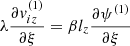
Appendix C: First-order equations
 (C.1)
(C.1)
 (C.2)
(C.2)
 (C.3)
(C.3)
 (C.4)
(C.4)
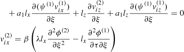
Appendix D: Second-order equations
 (D.1)
(D.1)
 (D.2)
(D.2)
 (D.3)
(D.3)
 (D.4)
(D.4)
 (D.5)
(D.5)
All Tables
Analytical profile parameters for embedded astrophysical structures and corresponding numerical values used in Figs. 1–6.
All Figures
|
Fig. 1. Contour plots of key ISM parameters in the local Galactic disk plane near embedded astronomical structures. The radii of the dashed magenta circles represent the characteristic size of the embedded structures. Panel (a): log10 of the total magnetic field strength, B0 (μG), featuring diamagnetic depletion in the H II region and shell-like compressions at the SWB and SNR. Panel (b): log10 of total ion number density, ni0 (cm−3). Panel (c): log10 of electron temperature Te0 (K). Panel (d): log10 of plasma β. High-β (β > 1) regions are masked in cyan, while ultra-low-β (β < me/mi) regions are masked in green. The H II region is centered at (R, Z)≈(4, 0) kpc, SWB at (7, 0) kpc, and SNR at (10, 0) kpc. Note that the background field in panel (a) is normalized to a microgauss scale to match the 1D profiles in Figs. 2 and 3. |
| In the text | |
|
Fig. 2. Detailed 1D profiles of ISM parameters through the center of the SWB. Panel (a): Total magnetic field B0 (μG), showing slight compression at the shell but minimal interior perturbation. Panel (b): Number densities (cm−3) for electrons (ne0; solid green), ions (ni0; dotted blue), and positrons (np0; dashed red). Note the deep central cavity where ion density drops significantly. Panel (c): Electron temperature, Te0 (K), exhibiting the characteristic “flat-top” plateau of the hot shocked wind (T ∼ 106 K). |
| In the text | |
|
Fig. 3. Detailed 1D profiles of ISM parameters through the center of the SNR. Panel (a): Total magnetic field, B0 (μG), highlighting the twin peaks of the shock-compressed shell and the central spike corresponding to the PWN. Panel (b): Multi-species densities (cm−3). The ion density (ni0; dotted blue) forms a shell but vanishes in the core, while the positron density (np0; dashed red) rises centrally, creating a pair-dominated interior. Panel (c): Electron temperature, Te0 (K), showing intense shock heating at the shell. |
| In the text | |
|
Fig. 4. 2D Galactic maps of KA soliton amplitude (ψ0; panel a) and width (W; panel b), at κe = 150, κp = 100, θ = 85°, U = −0.06, and σ = 1. The parameters for the background (WIM) and the analytical profiles of embedded structures are given in Tables B.1 and B.2, respectively. |
| In the text | |
|
Fig. 5. 1D profiles of plasma β (panel a), amplitude (panel b), and width (panel c) for Z = 0 kpc at the SWB for same parameters as in Fig. 4. |
| In the text | |
|
Fig. 6. 1D profiles of plasma β (panel a), amplitude (panel b), and width (panel c) for Z = 0 kpc at SNR for same parameters as in Fig. 4. |
| In the text | |
Current usage metrics show cumulative count of Article Views (full-text article views including HTML views, PDF and ePub downloads, according to the available data) and Abstracts Views on Vision4Press platform.
Data correspond to usage on the plateform after 2015. The current usage metrics is available 48-96 hours after online publication and is updated daily on week days.
Initial download of the metrics may take a while.