


| Issue |
A&A
Volume 711, July 2026
Euclid Quick Data Release (Q1)
|
|
|---|---|---|
| Article Number | A27 | |
| Number of page(s) | 20 | |
| Section | Extragalactic astronomy | |
| DOI | https://doi.org/10.1051/0004-6361/202554605 | |
| Published online | 30 June 2026 | |
Euclid Quick Data Release (Q1)
XXVII. The Strong Lensing Discovery Engine B – Early strong lens candidates from visual inspection of high-velocity dispersion galaxies
1
University of Applied Sciences and Arts of Northwestern Switzerland, School of Engineering, 5210 Windisch, Switzerland
2
Institute of Cosmology and Gravitation, University of Portsmouth, Portsmouth PO1 3FX, UK
3
Institute of Physics, Laboratory of Astrophysics, Ecole Polytechnique Fédérale de Lausanne (EPFL), Observatoire de Sauverny, 1290 Versoix, Switzerland
4
School of Mathematics, Statistics and Physics, Newcastle University, Herschel Building, Newcastle-upon-Tyne, NE1 7RU, UK
5
Jet Propulsion Laboratory, California Institute of Technology, 4800 Oak Grove Drive, Pasadena CA 91109, USA
6
Dipartimento di Fisica “Aldo Pontremoli”, Università degli Studi di Milano, Via Celoria 16, 20133 Milano, Italy
7
INAF-IASF Milano, Via Alfonso Corti 12, 20133 Milano, Italy
8
Dipartimento di Fisica e Astronomia “Augusto Righi” – Alma Mater Studiorum Università di Bologna, Via Piero Gobetti 93/2, 40129 Bologna, Italy
9
INAF-Osservatorio di Astrofisica e Scienza dello Spazio di Bologna, Via Piero Gobetti 93/3, 40129 Bologna, Italy
10
INFN-Sezione di Bologna, Viale Berti Pichat 6/2, 40127 Bologna, Italy
11
Max-Planck-Institut für Astrophysik, Karl-Schwarzschild-Str. 1, 85748 Garching, Germany
12
Technical University of Munich, TUM School of Natural Sciences, Physics Department, James-Franck-Str. 1, 85748 Garching, Germany
13
David A. Dunlap Department of Astronomy & Astrophysics, University of Toronto, 50 St George Street, Toronto Ontario M5S 3H4, Canada
14
Jodrell Bank Centre for Astrophysics, Department of Physics and Astronomy, University of Manchester, Oxford Road, Manchester M13 9PL, UK
15
Sydney Institute for Astronomy, School of Physics, University of Sydney, NSW 2006, Australia
16
SCITAS, Ecole Polytechnique Fédérale de Lausanne (EPFL), 1015 Lausanne, Switzerland
17
Institut de Ciències del Cosmos (ICCUB), Universitat de Barcelona (IEEC-UB), Martí i Franquès 1, 08028 Barcelona, Spain
18
Institució Catalana de Recerca i Estudis Avançats (ICREA), Passeig de Lluís Companys 23, 08010 Barcelona, Spain
19
Universitäts-Sternwarte München, Fakultät für Physik, Ludwig-Maximilians-Universität München, Scheinerstrasse 1, 81679 München, Germany
20
Max Planck Institute for Extraterrestrial Physics, Giessenbachstr. 1, 85748 Garching, Germany
21
Aix-Marseille Université, CNRS, CNES, LAM, Marseille, France
22
Institut d’Astrophysique de Paris, UMR 7095, CNRS, and Sorbonne Université, 98 bis boulevard Arago, 75014 Paris, France
23
MTA-CSFK Lendület Large-Scale Structure Research Group, Konkoly-Thege Miklós út 15-17, H-1121 Budapest, Hungary
24
Konkoly Observatory, HUN-REN CSFK, MTA Centre of Excellence, Budapest, Konkoly Thege Miklós út 15-17., H-1121, Hungary
25
School of Physical Sciences, The Open University, Milton Keynes, MK7 6AA, UK
26
STAR Institute, University of Liège, Quartier Agora, Allée du six Août 19c, 4000 Liège, Belgium
27
INAF-Osservatorio Astronomico di Capodimonte, Via Moiariello 16, 80131 Napoli, Italy
28
Department of Physics, Oxford University, Keble Road, Oxford OX1 3RH, UK
29
Department of Astronomy, University of Cape Town, Rondebosch, Cape Town, 7700, South Africa
30
Inter-University Institute for Data Intensive Astronomy, Department of Astronomy, University of Cape Town, 7701 Rondebosch, Cape Town, South Africa
31
INAF, Istituto di Radioastronomia, Via Piero Gobetti 101, 40129 Bologna, Italy
32
Université Paris-Saclay, CNRS, Institut d’astrophysique spatiale, 91405 Orsay, France
33
ESAC/ESA, Camino Bajo del Castillo, s/n., Urb. Villafranca del Castillo, 28692 Villanueva de la Cañada, Madrid, Spain
34
School of Mathematics and Physics, University of Surrey, Guildford, Surrey, GU2 7XH, UK
35
INAF-Osservatorio Astronomico di Brera, Via Brera 28, 20122 Milano, Italy
36
Université Paris-Saclay, Université Paris Cité, CEA, CNRS, AIM, 91191 Gif-sur-Yvette, France
37
IFPU, Institute for Fundamental Physics of the Universe, Via Beirut 2, 34151 Trieste, Italy
38
INAF-Osservatorio Astronomico di Trieste, Via G. B. Tiepolo 11, 34143 Trieste, Italy
39
INFN, Sezione di Trieste, Via Valerio 2, 34127 Trieste TS, Italy
40
SISSA, International School for Advanced Studies, Via Bonomea 265, 34136 Trieste TS, Italy
41
Dipartimento di Fisica e Astronomia, Università di Bologna, Via Gobetti 93/2, 40129 Bologna, Italy
42
INAF-Osservatorio Astronomico di Padova, Via dell’Osservatorio 5, 35122 Padova, Italy
43
Space Science Data Center, Italian Space Agency, Via del Politecnico snc, 00133 Roma, Italy
44
Dipartimento di Fisica, Università di Genova, Via Dodecaneso 33, 16146 Genova, Italy
45
INFN-Sezione di Genova, Via Dodecaneso 33, 16146 Genova, Italy
46
Department of Physics “E. Pancini”, University Federico II, Via Cinthia 6, 80126 Napoli, Italy
47
Instituto de Astrofísica e Ciências do Espaço, Universidade do Porto, CAUP, Rua das Estrelas, PT4150-762 Porto, Portugal
48
Faculdade de Ciências da Universidade do Porto, Rua do Campo de Alegre, 4150-007 Porto, Portugal
49
Dipartimento di Fisica, Università degli Studi di Torino, Via P. Giuria 1, 10125 Torino, Italy
50
INFN-Sezione di Torino, Via P. Giuria 1, 10125 Torino, Italy
51
INAF-Osservatorio Astrofisico di Torino, Via Osservatorio 20, 10025 Pino Torinese (TO), Italy
52
European Space Agency/ESTEC, Keplerlaan 1, 2201 AZ, Noordwijk, The Netherlands
53
Institute Lorentz, Leiden University, Niels Bohrweg 2, 2333 CA, Leiden, The Netherlands
54
Leiden Observatory, Leiden University, Einsteinweg 55, 2333 CC, Leiden, The Netherlands
55
INAF-Osservatorio Astronomico di Roma, Via Frascati 33, 00078 Monteporzio Catone, Italy
56
INFN-Sezione di Roma, Piazzale Aldo Moro, 2 – c/o Dipartimento di Fisica, Edificio G. Marconi, 00185 Roma, Italy
57
Centro de Investigaciones Energéticas, Medioambientales y Tecnológicas (CIEMAT), Avenida Complutense 40, 28040 Madrid, Spain
58
Port d’Informació Científica, Campus UAB, C. Albareda s/n, 08193 Bellaterra (Barcelona), Spain
59
Institute for Theoretical Particle Physics and Cosmology (TTK), RWTH Aachen University, 52056 Aachen, Germany
60
INFN section of Naples, Via Cinthia 6, 80126 Napoli, Italy
61
Institute for Astronomy, University of Hawaii, 2680 Woodlawn Drive, Honolulu, HI, 96822, USA
62
Dipartimento di Fisica e Astronomia “Augusto Righi” – Alma Mater Studiorum Università di Bologna, Viale Berti Pichat 6/2, 40127 Bologna, Italy
63
Instituto de Astrofísica de Canarias, Vía Láctea, 38205 La Laguna, Tenerife, Spain
64
Institute for Astronomy, University of Edinburgh, Royal Observatory, Blackford Hill, Edinburgh EH9 3HJ, UK
65
European Space Agency/ESRIN, Largo Galileo Galilei 1, 00044 Frascati, Roma, Italy
66
Université Claude Bernard Lyon 1, CNRS/IN2P3, IP2I Lyon, UMR 5822, Villeurbanne F-69100, France
67
UCB Lyon 1, CNRS/IN2P3, IUF, IP2I Lyon, 4 rue Enrico Fermi, 69622 Villeurbanne, France
68
Mullard Space Science Laboratory, University College London, Holmbury St Mary, Dorking, Surrey, RH5 6NT, UK
69
Departamento de Física, Faculdade de Ciências, Universidade de Lisboa, Edifício C8, Campo Grande, PT1749-016 Lisboa, Portugal
70
Instituto de Astrofísica e Ciências do Espaço, Faculdade de Ciências, Universidade de Lisboa, Campo Grande, 1749-016 Lisboa, Portugal
71
Department of Astronomy, University of Geneva, ch. d’Ecogia 16, 1290 Versoix, Switzerland
72
INAF-Istituto di Astrofisica e Planetologia Spaziali, Via del Fosso del Cavaliere, 100, 00100 Roma, Italy
73
Aix-Marseille Université, CNRS/IN2P3, CPPM, Marseille, France
74
INFN-Bologna, Via Irnerio 46, 40126 Bologna, Italy
75
School of Physics, HH Wills Physics Laboratory, University of Bristol, Tyndall Avenue, Bristol BS8 1TL, UK
76
FRACTAL S.L.N.E., calle Tulipán 2, Portal 13 1A, 28231 Las Rozas de Madrid, Spain
77
INFN-Sezione di Milano, Via Celoria 16, 20133 Milano, Italy
78
NRC Herzberg, 5071 West Saanich Rd, Victoria BC V9E 2E7, Canada
79
Institute of Theoretical Astrophysics, University of Oslo, P.O. Box 1029 Blindern, 0315 Oslo, Norway
80
Department of Physics, Lancaster University, Lancaster LA1 4YB, UK
81
Felix Hormuth Engineering, Goethestr. 17, 69181 Leimen, Germany
82
Technical University of Denmark, Elektrovej 327, 2800 Kgs. Lyngby, Denmark
83
Cosmic Dawn Center (DAWN), Denmark
84
Max-Planck-Institut für Astronomie, Königstuhl 17, 69117 Heidelberg, Germany
85
NASA Goddard Space Flight Center, Greenbelt MD 20771, USA
86
Department of Physics and Helsinki Institute of Physics, Gustaf Hällströmin katu 2, 00014 University of Helsinki, Finland
87
Université de Genève, Département de Physique Théorique and Centre for Astroparticle Physics, 24 quai Ernest-Ansermet, CH-1211 Genève 4, Switzerland
88
Department of Physics, P.O. Box 64, 00014 University of Helsinki, Finland
89
Helsinki Institute of Physics, Gustaf Hällströmin katu 2 University of Helsinki, Helsinki, Finland
90
Centre de Calcul de l’IN2P3/CNRS, 21 avenue Pierre de Coubertin, 69627 Villeurbanne Cedex, France
91
Laboratoire d’etude de l’Univers et des phenomenes eXtremes, Observatoire de Paris, Université PSL, Sorbonne Université, CNRS, 92190 Meudon, France
92
SKA Observatory, Jodrell Bank, Lower Withington, Macclesfield, Cheshire, SK11 9FT, UK
93
University of Applied Sciences and Arts of Northwestern Switzerland, School of Computer Science, 5210 Windisch, Switzerland
94
Universität Bonn, Argelander-Institut für Astronomie, Auf dem Hügel 71, 53121 Bonn, Germany
95
Department of Physics, Institute for Computational Cosmology, Durham University, South Road, Durham DH1 3LE, UK
96
Université Côte d’Azur, Observatoire de la Côte d’Azur, CNRS, Laboratoire Lagrange, Bd de l’Observatoire, CS 34229, 06304 Nice cedex 4, France
97
Université Paris Cité, CNRS, Astroparticule et Cosmologie, 75013 Paris, France
98
CNRS-UCB International Research Laboratory, Centre Pierre Binetruy, IRL2007, CPB-IN2P3, Berkeley, USA
99
Institut d’Astrophysique de Paris, 98bis Boulevard Arago, 75014 Paris, France
100
Aurora Technology for European Space Agency (ESA), Camino bajo del Castillo, s/n, Urbanizacion Villafranca del Castillo, Villanueva de la Cañada, 28692, Madrid, Spain
101
Institut de Física d’Altes Energies (IFAE), The Barcelona Institute of Science and Technology, Campus UAB, 08193 Bellaterra (Barcelona), Spain
102
DARK, Niels Bohr Institute, University of Copenhagen, Jagtvej 155, 2200 Copenhagen, Denmark
103
Waterloo Centre for Astrophysics, University of Waterloo, Waterloo Ontario N2L 3G1, Canada
104
Department of Physics and Astronomy, University of Waterloo, Waterloo Ontario N2L 3G1, Canada
105
Perimeter Institute for Theoretical Physics, Waterloo Ontario N2L 2Y5, Canada
106
Centre National d’Etudes Spatiales – Centre spatial de Toulouse, 18 avenue Edouard Belin, 31401 Toulouse Cedex 9, France
107
Institute of Space Science, Str. Atomistilor, nr. 409 Măgurele, Ilfov, 077125, Romania
108
Consejo Superior de Investigaciones Cientificas, Calle Serrano 117, 28006 Madrid, Spain
109
Universidad de La Laguna, Departamento de Astrofísica, 38206 La Laguna, Tenerife, Spain
110
Dipartimento di Fisica e Astronomia “G. Galilei”, Università di Padova, Via Marzolo 8, 35131 Padova, Italy
111
INFN-Padova, Via Marzolo 8, 35131 Padova, Italy
112
Institut für Theoretische Physik, University of Heidelberg, Philosophenweg 16, 69120 Heidelberg, Germany
113
Institut de Recherche en Astrophysique et Planétologie (IRAP), Université de Toulouse, CNRS, UPS, CNES, 14 Av. Edouard Belin, 31400 Toulouse, France
114
Université St Joseph; Faculty of Sciences, Beirut, Lebanon
115
Departamento de Física, FCFM, Universidad de Chile, Blanco Encalada 2008, Santiago, Chile
116
Universität Innsbruck, Institut für Astro- und Teilchenphysik, Technikerstr. 25/8, 6020 Innsbruck, Austria
117
Institut d’Estudis Espacials de Catalunya (IEEC), Edifici RDIT, Campus UPC, 08860 Castelldefels, Barcelona, Spain
118
Satlantis, University Science Park, Sede Bld, 48940 Leioa-Bilbao, Spain
119
Institute of Space Sciences (ICE, CSIC), Campus UAB, Carrer de Can Magrans, s/n, 08193 Barcelona, Spain
120
Instituto de Astrofísica e Ciências do Espaço, Faculdade de Ciências, Universidade de Lisboa, Tapada da Ajuda, 1349-018 Lisboa, Portugal
121
Cosmic Dawn Center (DAWN)
122
Niels Bohr Institute, University of Copenhagen, Jagtvej 128, 2200 Copenhagen, Denmark
123
Universidad Politécnica de Cartagena, Departamento de Electrónica y Tecnología de Computadoras, Plaza del Hospital 1, 30202 Cartagena, Spain
124
Kapteyn Astronomical Institute, University of Groningen, PO Box 800, 9700 AV, Groningen, The Netherlands
125
Infrared Processing and Analysis Center, California Institute of Technology, Pasadena CA 91125, USA
126
Dipartimento di Fisica e Scienze della Terra, Università degli Studi di Ferrara, Via Giuseppe Saragat 1, 44122 Ferrara, Italy
127
Istituto Nazionale di Fisica Nucleare, Sezione di Ferrara, Via Giuseppe Saragat 1, 44122 Ferrara, Italy
128
INAF – Osservatorio Astronomico di Brera, Via Emilio Bianchi 46, 23807 Merate, Italy
129
INAF-Osservatorio Astronomico di Brera, Via Brera 28, 20122 Milano, Italy, and INFN-Sezione di Genova, Via Dodecaneso 33, 16146 Genova, Italy
130
ICL, Junia, Université Catholique de Lille, LITL, 59000 Lille, France
131
ICSC – Centro Nazionale di Ricerca in High Performance Computing, Big Data e Quantum Computing, Via Magnanelli 2, Bologna, Italy
132
Instituto de Física Teórica UAM-CSIC, Campus de Cantoblanco, 28049 Madrid, Spain
133
CERCA/ISO, Department of Physics, Case Western Reserve University, 10900 Euclid Avenue, Cleveland OH 44106, USA
134
Laboratoire Univers et Théorie, Observatoire de Paris, Université PSL, Université Paris Cité, CNRS, 92190 Meudon, France
135
Departamento de Física Fundamental. Universidad de Salamanca., Plaza de la Merced s/n., 37008 Salamanca, Spain
136
Université de Strasbourg, CNRS, Observatoire astronomique de Strasbourg, UMR 7550, 67000 Strasbourg, France
137
Center for Data-Driven Discovery, Kavli IPMU (WPI), UTIAS, The University of Tokyo, Kashiwa, Chiba, 277-8583, Japan
138
California Institute of Technology, 1200 E California Blvd, Pasadena CA 91125, USA
139
Department of Physics & Astronomy, University of California Irvine, Irvine CA 92697, USA
140
Department of Mathematics and Physics E. De Giorgi, University of Salento, Via per Arnesano, CP-I93, 73100 Lecce, Italy
141
INFN, Sezione di Lecce, Via per Arnesano, CP-193, 73100 Lecce, Italy
142
INAF-Sezione di Lecce, c/o Dipartimento Matematica e Fisica, Via per Arnesano, 73100 Lecce, Italy
143
Departamento Física Aplicada, Universidad Politécnica de Cartagena, Campus Muralla del Mar, 30202 Cartagena, Murcia, Spain
144
Instituto de Física de Cantabria, Edificio Juan Jordá, Avenida de los Castros, 39005 Santander, Spain
145
CEA Saclay, DFR/IRFU, Service d’Astrophysique, Bat. 709, 91191 Gif-sur-Yvette, France
146
Department of Computer Science, Aalto University, PO Box 15400 Espoo FI-00 076, Finland
147
Instituto de Astrofísica de Canarias, c/ Via Lactea s/n, La Laguna 38200, Spain .
Departamento de Astrofísica de la Universidad de La Laguna, Avda. Francisco Sanchez, La Laguna, 38200, Spain
148
Ruhr University Bochum, Faculty of Physics and Astronomy, Astronomical Institute (AIRUB), German Centre for Cosmological Lensing (GCCL), 44780 Bochum, Germany
149
Department of Physics and Astronomy, University of Turku, Vesilinnantie 5, 20014 Turku, Finland
150
Serco for European Space Agency (ESA), Camino bajo del Castillo, s/n, Urbanizacion Villafranca del Castillo, Villanueva de la Cañada, 28692 Madrid, Spain
151
ARC Centre of Excellence for Dark Matter Particle Physics, Melbourne, Australia
152
Centre for Astrophysics & Supercomputing, Swinburne University of Technology, Hawthorn Victoria 3122, Australia
153
Department of Physics and Astronomy, University of the Western Cape, Bellville, Cape Town, 7535, South Africa
154
DAMTP, Centre for Mathematical Sciences, Wilberforce Road, Cambridge CB3 0WA, UK
155
Kavli Institute for Cosmology Cambridge, Madingley Road, Cambridge CB3 0HA, UK
156
Department of Astrophysics, University of Zurich, Winterthurerstrasse 190, 8057 Zurich, Switzerland
157
Department of Physics, Centre for Extragalactic Astronomy, Durham University, South Road, Durham DH1 3LE, UK
158
IRFU, CEA, Université Paris-Saclay, 91191 Gif-sur-Yvette Cedex, France
159
Oskar Klein Centre for Cosmoparticle Physics, Department of Physics, Stockholm University, Stockholm SE-106 91, Sweden
160
Astrophysics Group, Blackett Laboratory, Imperial College London, London SW7 2AZ, UK
161
Univ. Grenoble Alpes, CNRS, Grenoble INP, LPSC-IN2P3, 53, Avenue des Martyrs, 38000 Grenoble, France
162
INAF-Osservatorio Astrofisico di Arcetri, Largo E. Fermi 5, 50125 Firenze, Italy
163
Dipartimento di Fisica, Sapienza Università di Roma, Piazzale Aldo Moro 2, 00185 Roma, Italy
164
Centro de Astrofísica da Universidade do Porto, Rua das Estrelas, 4150-762 Porto, Portugal
165
HE Space for European Space Agency (ESA), Camino bajo del Castillo, s/n, Urbanizacion Villafranca del Castillo, Villanueva de la Cañada, 28692 Madrid, Spain
166
Dipartimento di Fisica – Sezione di Astronomia, Università di Trieste, Via Tiepolo 11, 34131 Trieste, Italy
167
Department of Astrophysical Sciences, Peyton Hall, Princeton University, Princeton NJ 08544, USA
168
Theoretical astrophysics, Department of Physics and Astronomy, Uppsala University, Box 516, 751 37 Uppsala, Sweden
169
Minnesota Institute for Astrophysics, University of Minnesota, 116 Church St SE, Minneapolis MN 55455, USA
170
Mathematical Institute, University of Leiden, Einsteinweg 55, 2333 CA, Leiden, The Netherlands
171
Institute of Astronomy, University of Cambridge, Madingley Road, Cambridge CB3 0HA, UK
172
Space physics and astronomy research unit, University of Oulu, Pentti Kaiteran katu 1, FI-90014 Oulu, Finland
173
Department of Physics and Astronomy, Lehman College of the CUNY, Bronx NY 10468, USA
174
American Museum of Natural History, Department of Astrophysics, New York, NY 10024, USA
175
Center for Computational Astrophysics, Flatiron Institute, 162 5th Avenue, New York, NY 10010, USA
176
Department of Physics and Astronomy, University of British Columbia, Vancouver BC V6T 1Z1, Canada
★ Corresponding author: This email address is being protected from spambots. You need JavaScript enabled to view it.
Received:
18
March
2025
Accepted:
24
July
2025
Abstract
We present a search for strong gravitational lenses in Euclid imaging with a high stellar velocity dispersion (σv > 180 km s−1) reported by SDSS and DESI. We performed expert visual inspection and classification of 11 660 Euclid images. We discovered 38 grade A and 40 grade B candidate lenses, which is consistent with an expected sample of ∼32. Palomar spectroscopy confirmed 5 lens systems, while DESI spectra confirmed one system, provided ambiguous results for another, and helped to discard a third system. The Euclid automated lens modeler modelled 53 candidates, confirmed 38 as lenses, failed to model 9, and ruled out 6 grade B candidates. For the remaining 25 candidates, we were unable to gather additional information. More importantly, our classified non-lenses provide an excellent training set for machine-learning lens classifiers. We created high-fidelity simulations of Euclid lenses by painting realistic lensed sources behind the tagged (non-lens) luminous red galaxies. This training set is the foundation stone for the Euclid galaxy-galaxy strong-lensing discovery engine.
Key words: gravitational lensing: strong / methods: statistical / catalogs
© The Authors 2026
 Open Access article, published by EDP Sciences, under the terms of the Creative Commons Attribution License (https://creativecommons.org/licenses/by/4.0), which permits unrestricted use, distribution, and reproduction in any medium, provided the original work is properly cited.
This article is published in open access under the Subscribe to Open model. This email address is being protected from spambots. You need JavaScript enabled to view it. to support open access publication.
1. Introduction
Strong gravitational lenses are powerful tools for understanding the most fundamental questions in astrophysics. They can be used to study key insights into the galaxy structure and cosmology (Shajib et al. 2021; Treu et al. 2022), to constrain the nature of gravity (Collett et al. 2018) and the expansion history of our Universe (Wells et al. 2024) and the most massive galaxies within it (Auger et al. 2009; Sonnenfeld 2024). Unfortunately, strong lenses are also rare. The typical deflection angle produced by a massive galaxy, assuming a spherical isothermal profile, is 1″ so that strong lensing is only observed when a background galaxy lies closer than this angular distance from the optical axis between the observer and the deflector.
The first multiply imaged gravitationally lensed quasar was discovered in 1979 (Walsh et al. 1979). Since then, ∼10 000 cases of strong gravitational-lensing candidates by galaxies have been detected, and examples of lensed galaxies (Jacobs et al. 2019; Petrillo et al. 2019; Cañameras et al. 2020; Li et al. 2020; Huang et al. 2021; Savary et al. 2022; Storfer et al. 2024; Acevedo Barroso et al. 2025), supernovae (Kelly et al. 2015; Goobar et al. 2017; Pierel et al. 2024), and even individual stars (Kelly et al. 2018; Welch et al. 2022; Meena et al. 2023) are now known. Based on this heterogeneous sample, a wide range of science has been conducted, but it has limited the statistical power of strong lensing.
The main barrier to expanding the sample of strong gravitational lenses is the need for a high angular resolution over a wide area of sky. Most galaxy lenses in the Universe have an Einstein radius of ∼0 5 (Collett 2015), and ground-based surveys (with a seeing of ∼1″) can therefore only hope to resolve multiple imaging around the most massive galaxies. Observations from space provide the angular resolution to resolve more typical galaxy-scale lenses, and ∼10 lenses can be discovered per square degree in Hubble Space Telescopeimaging (Faure et al. 2008; Garvin et al. 2022). The Visible Camera (VIS, Euclid Collaboration: Cropper et al. 2025) on Euclid (Euclid Collaboration: Mellier et al. 2025) will provide space-based imaging of over 14 000 deg2, and it thus offers a step change in the discovery potential of strong lenses. Forecasts by Collett (2015) showed that Euclid has the sensitivity to discover 170 000 strong lenses.
Euclid will detect 1.5 billion unlensed galaxies, and finding 170 000 strong lenses will therefore be a needle-in-a-haystack problem. It will be impossible to visually inspect every galaxy with such a large dataset, even though it has yielded large samples of lenses in smaller surveys (Jackson 2008; More et al. 2016; Acevedo Barroso et al. 2025). Machine-learning has become a powerful tool for pre-selecting strong-lens candidates (Jacobs et al. 2017, 2019; Petrillo et al. 2019; Li et al. 2020; Rojas et al. 2022), but even with a classifier that is accurate to 99.99%, false positives would dominate. Currently, citizen scientists (Marshall et al. 2015) or an even more accurate classifier are required to reduce the strong-lens sample to a tractable problem.
The Euclid Quick Release Q1 (2025) provides 63 deg2 of data that are representative of the full Euclid Wide Survey. This sample should contain ∼600 lenses (scaling from Collett 2015) and gives us the first opportunity to implement, test, and validate our lens-finding pipeline on a large scale. This paper is part of a series of papers that develop, describe, and demonstrate the Euclid strong-lens discovery pipeline on the Q1 dataset (Euclid Collaboration: Aussel et al. 2026).
This paper focuses on the visual inspection of spectroscopically selected massive galaxies with a high-velocity dispersion as observed by the Dark Energy Spectroscopic Instrument (DESI; DESI Collaboration 2024) and the Sloan Digital Sky Survey (SDSS; Kollmeier et al. 2019) carried out by experts in gravitational lensing. The cross-section for strong gravitational lensing scales as the velocity dispersion to the fourth power, and focusing on massive galaxies therefore maximises the chance of discovering new strong lenses before we train machine-learning classifiers. The velocity dispersion and redshift are the key parameters for understanding the deflection angles produced by massive galaxies (Treu & Koopmans 2004; Auger et al. 2009), and results from the spectroscopic sample will thus be easier to interpret.
Starting with a visual inspection of massive galaxies has three main benefits that enabled the machine-learning discoveries made in Euclid Collaboration: Walmsley et al. (2026). Firstly, it provides a training set of vetted non-lenses and a sample of non-lens massive galaxies that can be used to create a positive training set by painting lensed sources behind them. Secondly, it provides a small sample of real Euclid lenses that, in addition to their important scientific value, can be used to validate the performance of our machine-learning classifiers for recovering lenses in Euclid data. Finally, it allows us to determine whether Euclid is delivering on the strong-lensing forecast in Collett (2015).
The use of our simulated lenses to train machine-learning classifiers was described in Euclid Collaboration: Lines et al. (2026). The citizen-science inspection pipeline was described in Euclid Collaboration: Walmsley et al. (2026), where our main Q1 strong-lens sample was also reported. We reported our double-source plane lens-candidate sample in Euclid Collaboration: Li et al. (2026). In Euclid Collaboration: Holloway et al. (2026) we presented a machine-learning and visual inspection ensemble analysis.
This paper is organised as follows: In Sect. 2 we present our selection of the data we used, what we expect to find, and the design of the visual inspection, including the creation of the simulated test set. The results of the different visual inspection stages are reported in Sect. 3, as is the analysis of the performance on the simulated set. In Sect. 4 we present the results from spectroscopic follow-up, and in Sect. 5 we describe the results from the automatic modelling. Finally, in Sect. 6 we present updates for the simulation pipeline and their implementation to build a training sample for trained machine-learning models, and we analyse the selection function.
2. Data preparation and set-up
In this section, we present the design of our project, including the data selection, and we forecast what we expect to recover, which takes into account the initial selection, the stages of the visual inspection procedure, and a description of the procedure for creating simulations to evaluate the performance of the visual inspectors during the project.
2.1. Selecting massive galaxies spectroscopically
We selected massive galaxies with a velocity dispersion above 180 km s−1 from the DESI Early Data Release (EDR, DESI Collaboration 2024) and from the SDSS Data Release 18 (DR18, Almeida et al. 2023). In February 2024, we queried the Euclid Science Archive System (SAS) for any available product containing the selected targets. We found 11 560 out of ∼290 000 galaxies in the DESI sample and 100 out of 1.6 million in the SDSS sample. In Fig. 1 we present the redshift and velocity dispersion distribution of the sample that was available at this query date. Most of the galaxies were found in the performance verification (PV) data. The majority are in the Euclid Deep Field North (EDF-N), and a few are part of the COSMOS-wide field. This means that a few targets are outside the area that is covered by the Q1 release. For those targets, we present the latest available version in the SAS, and we call them pre-Q1 data. As we planned a visual inspection, the difference in the data processing between this and the final Euclid Q1 data was not especially relevant.
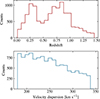 |
Fig. 1. Distribution of the redshift and velocity dispersion of the targets selected from DESI and SDSS with available Euclid data for the visual inspection. The distributions correspond to the pre-selection from two different surveys and to the availability in Euclid. |
2.2. Forecast of expected lenses
By pre-selecting only the galaxies with the highest velocity dispersion in DESI and SDSS, we selected galaxies with large strong-lensing cross-sections. This means that the prevalence of lensing should be much higher than for randomly selected galaxies. Collett (2015) used the LENSPOP to forecast the expected number of lenses in the entire Euclid survey, which is 170 000. This result is based on a population of singular isothermal ellipsoid (SIE) deflectors, whose velocity dispersions were drawn from the observed velocity dispersion function of galaxies (Choi et al. 2007) uniformly distributed in comoving volume between z = 0 and z = 2. Behind these deflectors lies a population of sources that were drawn from the LSST simulated catalogue (Connolly et al. 2010), and the sources have redshifts from 0 to 5.
We repurposed LENSPOP to forecast the expected number of our spectroscopically selected objects that should be detectable as lenses with Euclid. We replaced the LENSPOP deflector population with the observed redshift and velocity dispersions of our 11 660 targets, assuming they are all SIEs. We retained the LENSPOP background source population, the simulation of Euclid observations, and the criteria for discoverable lenses that were used by Collett (2015) (see this publication for further details). By applying this method, we expect that 32 lens systems should be discoverable from our 11 660 targets.
This estimate is far from perfect because it neglects any contribution to the lensing mass from groups, and it assumes that the DESI and SDSS velocity dispersions are correct, which is unlikely to be true for mergers. It also ignores any differences between our selection function and that of Collett (2015), who assumed a search on lens-subtracted IE band images. We used the IE and infrared bands, but did not subtract the lens light. The statistical errors of ∼10% on the velocity dispersion are irrelevant compared to these systematics.
This forecast may also not be accurate because it neglects the DESI and SDSS spectroscopic selection functions. A bright lensed arc will change the overall magnitude and colours of the system, which may decrease (or increase) the probability of DESI or SDSS targeting the system. In summary, we expect about 30 lenses, but it would not be surprising if the true number deviated by a factor of 5 in either direction.
2.3. Design of the visual inspection
To perform our visual inspection, we used a slightly modified version of the visualisation tool developed by Acevedo Barroso et al. (2025). We used only the one-by-one sequential viewer, which displays a target cutout in the IE band (Euclid Collaboration: Cropper et al. 2025) and two-colour composites using IE-YE-HE and YE-JE-HE (Euclid Collaboration: Jahnke et al. 2025). We added or modified the classification and subclassification buttons according to the different stages of this project. The final version of the classifier has three main buttons for the lensing classification: Lens (L), Possible Lens (PL), and Non Lens (NL), and six buttons for the morphological classification: Merger, Spiral, Ring, LRG, Simulation, and Other.
To achieve the goals of this project, we designed three stages. A beta stage for testing and for building a test set for the following stage, stage-1 for the detailed morphological classification, and stage-2 for the lens grading. These stages are detailed below.
In the beta stage, we aimed to test the modifications that we applied to the visualisation tool, but also to build a small test set for the following stage. To do this, six visual inspectors classified 2000 random targets from the whole sample. The classifiers were asked to use all the buttons for testing purposes, but the main focus was the identification of luminous red galaxies (LRGs) to build a test set that contained simulated lens systems based on real images, as explained in detail in Sect. 2.5, and LRGs as negative examples. Based on this stage, we identified 700 LRGs without any lensing features. We then created simulations and kept a fraction of the LRGs as negative examples. We constructed the test set such that visual inspectors should see a lens in every 10th to 15th image. This does not represent the real rate of lenses (∼1 in 1000 galaxies), but was meant to keep inspectors motivated.
In stage 1 we separated the sample into six groups, each with five visual inspectors. Each person received a sample of about 2100 targets mixed with a test set of 200 labelled targets, 150 simulations, and 50 LRGs, prepared with the information obtained in the beta test. This test set was the same for all individuals and had the purpose of detecting classifiers with poor completeness and purity that might bias the classification. The task in this stage was a detailed morphological classification, in which each galaxy was classified by clicking in the respective button according to the categories Merger, Spiral, Ring, LRG, and Other, which are the most common contaminants in lens searches. In the option Other, we expected users to classify any other type of galaxy that was not listed in the options, but also small galaxies for which insufficient detail made an accurate classification impossible. Furthermore, inspectors were instructed to identify lens candidates using the options: Lens, Possible Lens, and Simulation. We expected Lens to be used for obvious lens systems and Possible Lens for more doubtful ones, but no specific guidelines were given regarding the use of these buttons. The button Simulation was introduced for those who wished to test their abilities to distinguish simulations from real lens systems, but its use was not mandatory, and for the final grading, their votes counted as Lens.
Stage-2 was designed to grade all the possible lens systems. All visual inspectors here re-inspected all targets that received at least one vote in the categories Lens and Possible lens during stage-1. Each inspector received the same set of data (the collection of Lens and Possible lens) along with a new test set that was different from stage-1 and was built with the labels collected in the first stage. This time, the test set contained 111 simulations, so that the inspectors saw a lens every ∼10 images, and 80 non-lenses that were divided equally into four categories: LRGs, mergers, rings, and spirals. The purpose of this simulation set was not only to identify underperforming classifiers, but also to evaluate the selection function. The simulations were carefully designed to almost evenly sample the parameter space of the Einstein radii and the S/N of the lensed images. In this stage, the task was to classify the targets into Lens, Possible Lens, Non Lens, and Simulation, and this last category was optional. As in stage-1, non-specific guidelines were given, but we expected that inspectors would click Lens when an obvious lens system was displayed, Possible Lens when the system might be a lens, and Non Lens when no sign of lensing features was present.
2.4. Catalogues and score system
In order to create the final galaxy catalogues in the categories Spirals, Mergers, and Rings, we kept any object that received a vote in the respective category from at least three out of the four to five inspectors. For LRGs we increased this cut to two votes out of four to five because LRGs are typically not mistaken as any other category. Additional details of this morphological classification are provided in Sect. 3.1.
We tried two score systems for the lenses, a linear and a weighted system. In the linear system, we assigned a linear score to the three categories from 3 to 1 with L = 3, PL = 2, and NL = 1, and we then averaged among the number of participants. In the weighted system, we counted the votes for Lens three times more than the votes for Possible Lens. For our particular case, we observed that using the weighted score system separated the sample more clearly. This resulted in a different scoring system than the one used by Euclid Collaboration: Walmsley et al. (2026). The equation to obtain the visual inspection score of each target was
 (1)
(1)
where NL is the number of votes in the Lens category, and NPL is the number in the Possible Lens category. With this scoring system, each lens received a unique score between 3 and 0. That is, the higher the score, the more confident inspectors were that the system was a lens. We decided to make two cuts in the scores for the final lens catalogue to separate the candidates into two groups. Category A contained a group of candidates that was mainly comprised of obvious lens systems, with clear lens features. This was voted for most by the inspectors. Category B contained a group of candidates with more doubtful lens systems. Any target that did not pass the two cuts was discarded. The VI score thresholds for these categories are discussed in Sect. 3.2.
2.5. Simulations
To create the simulations, we used all four Euclid bands following the procedure described by Rojas et al. (2022), and we used Lenstronomy1 (Birrer & Amara 2018; Birrer et al. 2021). A summary of this procedure, along with the adaptations for Euclid data, is presented below.
Our deflectors were selected LRGs with known redshifts and velocity dispersions. We fit a Sérsic profile to the JE band image to obtain the ellipticity and central position of the galaxy, we used these parameters to create our mass model. To minimise the log-likelihood in this fitting procedure, we used a downhill simplex optimisation (Nelder & Mead 1965) with 500 maximum iterations. We were not interested in a perfect fit, but in a rough and fast estimation, and we therefore allowed some errors that might lead to a more diverse population of lenses.
We selected sources to act as background galaxies from the HST/ACS F814W high-resolution (Leauthaud et al. 2007; Scoville et al. 2007; Koekemoer et al. 2007) catalogue compiled by Cañameras et al. (2020). These are HST/HSC combined sources, where the image comes from the HST and the colour information from Hyper Suprime Cam (HSC) ultra-deep stack images (Aihara et al. 2018). In this case, we used the HST image and assigned a similar magnitude to match the Euclid filters. In the case of IE band, we used a combination of images with HSC r- band + i-band magnitudes. To match the infrared bands, we used the Ilbert et al. (2008) catalogue to assign infrared magnitudes to our source galaxies. To do this, we selected the source with the nearest gri magnitudes to ours and assigned their infrared magnitudes. In this case, the closest available infrared filters in the catalogue to the Euclid YE, JE, and HE filters are the z, J, and K bands, respectively. This resulted in some cases with obviously mismatched colours when displayed in colour-composite images, such as purplish lensing features.
When the lens and source data were both ready, we matched them in a way to ensure that they formed Einstein radii greater than 0 5. To do this, we calculated the minimum redshift that a source should have to produce an Einstein radius of 0
 5, and we selected a random source from the sources with a redshift above this value. We did not constrain the maximum Einstein radius because a system with such a large separation is rarely formed, and therefore, we allowed for this to happen.
After we had a lens-source pair, we created an SIE mass model, whose parameters were the Einstein radius, θE, position angle, the axis ratio, and the central position. We derived the Einstein radius using the lens and source redshifts and the velocity dispersion of the lens. The position angle, axis ratio, and central position were obtained from the Sérsic profile fitted to the lens. We used this mass model to lens the light of the background source, whose position was randomly selected within a square that enclosed the caustics. We downsampled the lensed source image to match the pixel size of the lens. Then, we convolved the image with a Gaussian with an FWHM of 0 15 for images in the IE filter or 0
 3 for those in the infrared to broadly mimic the effect that the telescope PSF could produce, although these values do not match the exact FWHM of the PSFs in each filter. Finally, we re-scaled the flux to the lens-image values. In Fig. 2 we show examples of simulations ranging over different combinations of Einstein radii and signal-to-noise ratio (S/N) of the source galaxy in the IE image. The S/N was calculated taking the maximum value of the quotient between the cumulative sum of the pixels in the lensed source image before adding it to the lens galaxy image, and the cumulative sum of the root mean square of the background standard deviation in the simulated image. This can be expressed as
 (2)
(2)
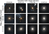 |
Fig. 2. Twelve example simulations selected to span different Einstein radii and log10(S/N) in the IE band. The size of each cutout is 10″ × 10″ and is displayed using an MTF function using the IE and YE bands. |
where Ii↓(xi, yi) denotes the pixel intensity at the position (x, y), and σi↓(xi, yi) is the background standard deviation at each pixel, both sorted in descending order of pixel S/N (Ii/σi). The function was evaluated for k between one and the number of pixels in the simulated image. The images are displayed using the midtone-transfer function (MTF; see Euclid Collaboration: Walmsley et al. 2026).
3. Results
Our visual inspection had three stages. A beta test, and two main steps: stage-1 and stage-2. In this section, we present the results for these two main stages.
3.1. Stage 1: Morphological visual classification
In stage-1 a total of 28 experts subscribed to perform the visual inspection. They were divided into six groups, four groups of five classifiers, and two groups of four classifiers. We ensured that each group had at least one experienced classifier, a person who had participated in several visual inspections before, to prevent doubtful or pessimistic classifiers from biasing the sample. The inspectors had three weeks to complete the task, and after the deadline, 25 participants returned classifications. To ensure at least four to five classifications per group, classifier K.R. inspected an additional three batches of data, and we thus kept the original split of four groups with five classifications and two groups with four classifications.
Based on the test set, the performance of all classifiers varied in completeness above 50% and purity above 97%, except for one, whose completeness and purity were both below 50%. Therefore, we decided not to use the classifications of this user. This finally left us with three groups with five classification and three groups with four classifications.
To analyse the morphological classification, we counted the votes in each category received by a target. To consider a target to be in the categories LRG, Spiral, Merger, Ring and Other, we applied the following requirements: The targets must have at least three votes in the corresponding category, and the target should have no vote in a lensing-related category. We wished to have a very clean sample of LRGs to use them for simulations, and we therefore added the restriction that it should not have any votes in one of the other categories to remove possible confusing targets. As a result, we obtained 2578 spirals, 250 merges, 61 rings, and 2477 galaxies in the category Others. In the case of LRGs, 16% of the sample that complied with the general requirements did not pass the additional restriction, which left a sample of 2798 secure LRGs. Only 0.7% of the whole sample did not receive any classification in any category by any user. The main cause of this were targets without IE band information or artefacts in the image that prevented a proper classification. Confusing results were obtained for 23% of the sample because the minimum of three votes in one category was not reached. These targets were not considered further. Examples of the best-classified targets in these categories are shown in Fig. 3. One remark regarding the category Other and Spiral was noted in a post-classification survey, where some inspectors mentioned that they classified edge-on spirals as spirals and other inspectors classified them in the category Others. This type of galaxy can therefore be found in both these categories.
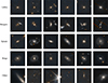 |
Fig. 3. Six examples of the targets classified in the LRG, mergers, spirals, rings, and other categories during stage-1 of the visual inspection. The size of the cut-outs is 15″ × 15″, and they are displayed using an MTF function using the IE and YE bands. |
Of the strong-lensing candidates, 1076 targets received at least one vote in one of the lensing-related categories, including 14 targets with at least three votes as Lens and 84 as Possible lens. Interestingly, 34 real targets were flagged by at least one person in the option Simulation.
3.2. Stage 2: Grading of the lens candidates
All visual inspectors who completed stage-1 were invited to participate in stage-2. After two weeks, all but one returned classifications of all targets. In this stage, we reclassified the 1076 targets with at least one vote in a lensing category from stage-1 based on the lensing-related options alone.
The user performance was evaluated using a different test set than the one used in stage 1. This updated set included simulations made with the previously classified LRGs and examples of different false positives. Most visual inspectors achieved a purity higher than 95% and a completeness higher than 70%. Three classifiers reached a purity lower than 80%, however, and one had a completeness lower than 50%. Consequently, we decided to exclude the classifications of these four visual inspectors from our final analysis.
We calculated individual scores for each target following Eq. (1). By plotting all targets and their scores, we visually decided to separate the targets into three categories, A, B, and Non-lens. The distinction between A and B can be seen as targets in category A are almost secure lens systems, while category B includes possible lens candidates and a few contaminants. For category A, we obtained 36 targets with a score above 1.20, and category B contained 40 targets with scores between 1.20 and 0.70. The remaining targets were discarded. In Figs. 4 and 5 we show all lens candidates separated by category, their score, and the data release availability (Q1 or pre-Q1). In Tables A.1 and A.2 we present the list of candidates in each category, their names, coordinates, redshifts, velocity dispersion, visual inspection score, and references to the discovery publication if they were previously detected.
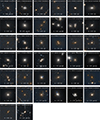 |
Fig. 4. Lens candidates in category A. Each image displays the lens candidate name at the top and the category, VI score, and data release at the bottom. The size of each cut-out is 15″ × 15″, and they are displayed using an MTF function using the IE and YE bands. |
4. Spectroscopic follow-up
In this section, we present the spectroscopic analysis of observations from the Palomar Observatory and the inspection of publicly available spectra from the DESI and SDSS archives in our search for emission or absorption lines at a redshift different from that of the reported lens. This might provide an estimate of the source redshift.
4.1. Palomar observations
We obtained optical spectroscopic follow-up of 12 category A candidates in the EDFN using the Double Spectrograph (DBSP, Oke & Gunn 1982) on the 5 m Hale telescope at Palomar Observatory between July and September 2024. Table A.3 presents the targets for which we were able to measure at least one redshift in the possible strong-lens system. The seeing in all nights ranged from 1 1 to 1
 5; most observations were obtained with ∼1
 3 seeing. Half the nights were photometric, meaning no cloud coverage, and the other half had variable levels of cloud coverage from minimal to sufficiently severe, and opaque monsoon clouds that caused the dome to be shuttered. For each source, we obtained two or three exposures of 1200 s using the 1
 5 slit, the 600 line blue grating (blazed at 4000 Å), the 5500 Å dichroic, and the 316 line red grating (blazed at 7500 Å). The slits were aligned on the candidate lensing galaxy at a position angle to cover the putative lensed source feature. The data were reduced using standard techniques within Image Reduction and Analysis Facility (IRAF), and the quality (Q) of the spectroscopic redshifts was assessed as either quality A, implying multiple detected features and a highly secure redshift, or quality B, implying some ambiguity to the reported redshift either as a result of the robustness of the putative detected feature or of ambiguity in the identification of that feature.
All the lensing galaxies proved to be early-type galaxies with Ca II H & K absorption and, generally, strong 4000 Å breaks. We obtained quality A redshifts for four lensed sources, all at z ∼ 2, as well as one quality B redshift at z = 2.316 (Fig. 6). In most cases, the lensed background source was revealed as a slightly offset or extended blue emission line coincident with the early-type lensing galaxy. Since the emission features did not correspond to any strong redshifted spectral features in early-type galaxies (which generally do not have emission lines), the most plausible identifications were lensed Lyα lines at z ∼ 2. One lensed source, EUCL J175555.21+635718.7, does not show Lyα emission, but instead shows the classic spectrum of a Lyman-break galaxy with multiple absorption lines due to the interstellar medium. A detailed analysis and further follow-up of this target and of EUCL J174907.29+645946.3, a possible double-source plane candidate, will be presented in Moustakas et al. (in prep.).
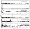 |
Fig. 6. Spectra of the five targets with source redshift estimates. The identified spectral lines are labeled, and the emission lines are indicated at the top of the image and the absorption lines at the bottom. The lines associated with the lens galaxy are shown as dashed red, and those corresponding to the source are plotted as dotted blue. |
4.2. Additional available spectra
We visually inspected the available DESI and SDSS spectra for all 78 targets. We found that all ten redshifts for the lens galaxies obtained from Palomar agree with the redshifts reported previously. The Lyα emission line for most source detections from Palomar is beyond the DESI spectra coverage or very near to the edge, which makes its detection in DESI data impossible or unreliable. Additional spectral features were identified in only four targets, including the EUCL J175555.21+635718.7, the Lyman-break galaxy mentioned above. Based on insights from Palomar spectroscopic data, the emission or absorption lines in many cases may probably lie beyond the observed spectral range or near the edges, where the noise levels are high. This makes a detection challenging. Additionally, the integration time may not have been sufficient to capture the often faint signals from the sources. The findings for the three additional detected targets are described below.
For EUCL J174613.92+662840.2, we found an emission line at 8587 Å. Based on its shape, it is likely O II, which corresponds to a source redshift of 1.303.
In the spectra of EUCL J100101.01+022036.5, we identified weak emission features at 7217 Å, 9603 Å, and 9693 Å, which might correspond to the O II and OIII] doublet and would indicate a source galaxy at z ∼ 0.935. The signal is weak, however, and this detection remains ambiguous.
The candidate EUCL J180152.75+655455.5 exhibits a clear set of emission lines at a different redshift than the absorptions lines corresponding to the lens (z = 0.36). We identified O II, Hβ, the OIII] doublet, and Hα, corresponding to a z ∼ 0.48. The close proximity of these two galaxies suggests that this system is not a strong-lens candidate.
5. Lens modelling
The Euclid strong-lens modelling pipeline (Nightingale in prep.) was applied to the 53 lens candidates with Q1 data, 24 category A, and 29 category B. This final step aimed to provide insights to assess whether the candidates are potential strong-lensing systems.
5.1. Approach
We performed an automated strong-lens modelling of all the candidates with Q1 available data using the Euclid strong-lens modelling pipeline2, adapted from the lens-modelling software PyAutoLens3 (Nightingale et al. 2021).
The lens mass was modelled as an isothermal profile,
 (3)
(3)
where  is the Einstein radius. The deflection angles were calculated using Tessore & Metcalf (2015)’s method in PyAutoLens. External shear was included, parametrised as (γ1ext, γ2ext), with the shear magnitude and orientation given by
 (4)
(4)
The deflection angles due to the external shear were computed analytically.
The Euclid strong-lens modelling pipeline models the light of the lens galaxy using a multi-Gaussian expansion (MGE; He et al. 2024), accounts for PSF blurring, and subtracts this model from the observed image. A mass model (isothermal distribution) ray-traces image pixels to the source plane, where a pixelised source reconstruction is performed using an adaptive Delaunay mesh. The pipeline iteratively fits various combinations of light, mass, and source models; the pipeline initially fits a simpler model using an MGE source for an efficient and robust convergence towards accurate results, and then, subsequent stages employ the more complex Voronoi source reconstruction. The pipeline chains five lens-model fits together in total.
For a further description of PyAutoLens, we refer to He et al. (2024), Nightingale et al. (2024), and Nightingale (in prep.) for full details. We also provide more details in Euclid Collaboration: Walmsley et al. (2026) Appendix A.
5.2. Modelling results
The first step assessed whether the automated modelling was successful, based primarily on how well the model reproduced the observed lensed source emission. The critical curves of the mass model and the source plane were also evaluated. A successful lens model does not necessarily confirm the candidate as a strong lens, but indicates that the model fit the data as expected. For instance, if the observed emission in the image-plane is singly imaged without a counter-image and the model reflects this, the fit is deemed successful, even though the candidate is not a strong lens. Overall, 44 out of 53 candidates (83%) were successfully modelled. The top row of Fig. 7 shows an example of a successful lens model fit.
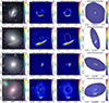 |
Fig. 7. PyAutoLens lens modelling. It informs the judgement of whether candidates are lenses. The first column shows the postage-stamp RGB cut-out image of each lens, the second column shows a clean foreground-subtracted image from the lens model multi-Gaussian expansion, the third column shows the model lensed source in the image plane, and the fourth column shows the source-plane reconstructions. The white and yellow curves represent tangential and radial critical curves and caustics. The top row shows a successful lens model fit, which traces the multiple images of the lensed source into a single region of the source plane, consistent with a strong-lens model. The remaining three rows show lens models that rule out the lensing hypothesis because they do not show evidence for multiple images or faint source galaxy emission near the centre of the candidate lens galaxy. This ruled out six candidates in total. |
For the 44 successful fits, the experts evaluated whether the candidates were genuine strong lenses based on the models. Of these, 38 were classified as strong lenses, and 6 were determined not to be. The second, third, and fourth rows of Fig. 7 show three examples of these 6 lenses, where the foreground lens light-subtracted image shows no sign of a counter-image, and the lensed source model does not predict one. All six non-lenses belonged to category B, including EUCL J180152.75+655455.5, which was blindly ruled out by this pipeline. This decision was later supported by a redshift estimation of the two galaxies (Sect. 4.2, z1 = 0.36 and z2 = 0.48), which confirmed that this is not a strong-lensing interaction. In Tables A.1 and A.2 we present the model success and the decision of the experts for each candidate. When the model fitted the system successfully and the classifiers agreed that the candidate was a lens, we also report the Einstein radii (θE).
6. Discussion
We morphologically categorised about 5000 galaxies that were discovered around 70 lens candidates, conducted a spectroscopic campaign at the Palomar Observatory to confirm 5 of them, and successfully automatically modelled 44 galaxies. In this section, we discuss the lensing selection function and how we used our results to build the training set that we used in Euclid Collaboration: Walmsley et al. (2026) and Euclid Collaboration: Lines et al. (2026).
6.1. Lensing selection function
The simulations in the test set we used in stage-2 provide broad but not exhaustive insight into our selection function. In Fig. 8 we present each simulation alongside its corresponding visual inspection score, mapped within the parameter space of the Einstein radii and the S/N of the lensed source in the IE band. To better understand the relation between these parameters and the visual inspection score, we used a Gaussian-process regressor (GPR) from the scikit-learn library (Pedregosa et al. 2011). The GPR allowed us to predict scores across the parameter range, and therefore, to understand the pattern in the data to model it and account for uncertainties. To do this, we used a composite kernel consisting of a ConstantKernel that represents the overall scale of the parameter function, a MaternKernel that provides flexibility in modelling smooth variations, and a WhiteKernel that accounts for noise in the data. We used the GPR to predict scores across the Einstein radii and the S/N range. This allowed us to create contour levels that provide a broad approximation of the expected score for each lens based on the S/N and Einstein radius alone. With this, we identified the regions of simulated lenses in which we successfully classified lens candidates versus those where they are missed.
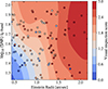 |
Fig. 8. Visual inspection score related to the Einstein radii and log10(S/N) of the lensed source in IE band. The colour maps represent the VI score, and the colour transition point from red to blue was set at 1.2 because this is the visual inspection score cut for candidates in category A. Red shaded areas therefore represent a region in which we can recover category A lens candidates, and blue shaded ares represent a region in which we struggle as visual inspectors to properly recognise or miss lens candidates. |
Based on the simulations, we predict that most of our highly scored candidates will have a high S/N and large Einstein radii, while systems with low S/N and small Einstein radii are the most likely to be missed by visual inspectors. This prediction is confirmed when we analyse the model parameters of our lens candidates, although we have much sparser coverage. The Einstein radius distribution of our candidates peaks at 1″ (see Fig. 9), but we recall that we preselected galaxies with a high-velocity dispersion, which makes configurations with a small Einstein radius less probable. The trend for the S/N is clear: A higher S/N correlates with higher visual inspection scores, and thus, with a greater probability of being recognised by visual inspectors. This is expected because a higher S/N ensures that the lensing features are visible, but it also highlights the limitations of human visual inspection. These results agree with our expectations because systems with a low S/N or a small Einstein radius pose significant challenges for human visual inspection (Rojas et al. 2022). Fig. 9 clearly shows, however, that the sample does not perfectly match what was predicted by LENSPOP: The Einstein radii are slightly smaller, and the arcs are substantially brighter. The difference in Einstein radius might be explained by the fact that we neglected the uncertainties in the observed velocity dispersions. There are far more low-mass galaxies that could scatter up from below our 180 km s−1 cut than go in the other direction. The brighter-than-expected VIS arc magnitudes indicate that the definition of a discoverable lens and the source population in LENSPOP are systematically incorrect. The total number of lenses we discovered is comparable to the ∼30 predicted in Sect. 2.2, which suggests that these effects cancel out to some extent, however.
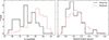 |
Fig. 9. IE magnitude of the lensed source and Einstein radius distributions of the lens candidates obtained after the automatic lens modeling (black) and LENSPOP predicted population, given the redshift and velocity dispersions of our initial sample (red). |
6.2. A training set for machine learning
In this section, we present some of the training samples we used for the machine-learning models and visual inspection projects run in Q1, with a special emphasis on the improvements we implemented in the simulation procedure.
Data-driven simulations are a powerful set to train machine-learning models and also test the performance of humans involved in visual inspections projects. To benefit, simulations need to be realistic enough to teach the correct properties to neural networks and to convince the human eye. For Q1, we therefore worked on two main improvements compared with the dataset presented during the visual inspection project described here: better information matching Euclid infrared bands for source magnitudes, and using the corresponding PSF.
First, to properly match the magnitudes of the sources in the infrared bands, we used the COSMOS 2020 (Weaver et al. 2022) catalogue and followed the same procedure as before, but this time, we used the VISTA Y, J, H-bands to match the Euclid YE, JE, HE bands. This resulted in a more realistic colour-composite version of the simulations.
Secondly, to transform the lensed source image into the Euclid properties, we used the modelled PSF from the Euclid pipeline for each cutout where we added a lensed source instead of using a circular Gaussian to mimic the effect of the PSF. This resulted in a lensed source that better matched the properties of the Euclid image and prevented us from creating unrealistic lensing sources that are too sharp or too smooth.
A total of 2585 LRGs that were categorised during stage-1 had Q1 available data. We used this sample to perform our new Q1 simulations. Additionally, to provide a larger training set, we rotated each LRG image by 90 degrees and paired it with a different source to produce a unique new simulations. This method was applied successfully before by Schuldt et al. (2021, 2023). With this method, we quadrupled the original set and provided a final training set with about 10 000 examples.
These new simulations as well as the catalogues of spirals, rings, mergers, and other previously classified in this work were used to train different machine-learning models (Euclid Collaboration: Walmsley et al. 2026; Euclid Collaboration: Lines et al. 2026). Simulations were also used to understand the selection function in the expert visual inspection and citizen-science projects carried out in the Q1 lens-finding project (Euclid Collaboration: Walmsley et al. 2026; Euclid Collaboration: Holloway et al. 2026). In Fig. 10 we present some examples of these simulations based on Q1 data, which span a wider range than those created in stage-2.
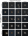 |
Fig. 10. Example of simulations following the new procedure. The 20 simulations are an example of a target in a different range of an Einstein radius and log10(S/N) in IE band. The size of each cut-out is 15″ × 15″, and they are displayed using an MTF function using the IE and YE bands. |
7. Conclusion
We have shown that the visual inspection of high-velocity dispersion galaxies is an efficient route to discoveri large numbers of lenses, without the need for machine-learning assistance.
We inspected 11 660 images and discovered 38 grade A and 40 grade B lenses. This is substantially more than were discovered in the untargeted inspection of Euclid ERO data, which found 3 grade A and 13 grade B lenses in 12 086 images (Acevedo Barroso et al. 2025). Unlike an untargeted search, our approach will always miss low-velocity dispersion lenses and lenses without spectroscopy, but it is substantially more efficient at finding lenses per human inspection.
We have six spectroscopically confirmed candidates. From the Palomar Observatory, we obtained the source redshift for five lens systems. From DESI and SDSS, we have redshifts for all the lens candidates, and we have an additional redshift for one source from DESI.
The expected number of lenses in our sample was 32 (with substantial uncertainties), based on modifications of the forecasts of Collett (2015). It is not clear whether we found more candidates due to shot noise or because the forecasts neglected the lensing cross-section boost of group and cluster haloes, or if the galaxy-galaxy lens rates are intrinsically higher than predicted by the model of Collett (2015). Our sample is clearly unlikely to be highly impure, however. All of the 21 grade A lenses for which the Euclid automated lens modeller ran successfully (Nightingale et al. 2021) were confirmed as lenses. Seventeen grade B lenses were confirmed as lenses, and six were excluded. The failure of the automatic modeller for the remaining candidates is not evidence that they are not lenses because the modeller can fail on true lenses due to group-scale haloes or contamination by foreground light.
Our approach cannot easily be scaled up to larger samples: DESI DR1 and Euclid DR1 are not expected to overlap substantially, and the visual inspection effort needed would be substantial even if we were to wait for the full datasets from both surveys.
An equally important aspect of our approach was to label a large sample of common false positives in machine-learning based strong-lens searches and to produce a sample of LRGs with known redshift and velocity dispersions that can be used to make a large sample of high-fidelity simulations of lenses by painting sources behind them. This result was a success and enabled us to produce a sample of 10 000 realistically simulated Euclid images of lenses and 5366 false positives broken into subclassifications of spiral, ring galaxy, merger, and other.
We have been successful in establishing a viable training set for machine learning. Five teams trained using our sample (Euclid Collaboration: Lines et al. 2026) and enabled citizen scientists and experts to efficiently discover 246 grade A and 254 grade B lenses (Euclid Collaboration: Walmsley et al. 2026). This galaxy-galaxy strong-lensing discovery engine is ready to discover over 100 000 strong lenses in the full Euclid dataset. The visual inspection of spectroscopically selected lenses is the foundation stone of the Euclid strong-lensing revolution.
Acknowledgments
The Euclid Consortium acknowledges the European Space Agency and a number of agencies and institutes that have supported the development of Euclid, in particular the Agenzia Spaziale Italiana, the Austrian Forschungsförderungsgesellschaft funded through BMK, the Belgian Science Policy, the Canadian Euclid Consortium, the Deutsches Zentrum für Luft- und Raumfahrt, the DTU Space and the Niels Bohr Institute in Denmark, the French Centre National d’Etudes Spatiales, the Fundação para a Ciência e a Tecnologia, the Hungarian Academy of Sciences, the Ministerio de Ciencia, Innovación y Universidades, the National Aeronautics and Space Administration, the National Astronomical Observatory of Japan, the Netherlandse Onderzoekschool Voor Astronomie, the Norwegian Space Agency, the Research Council of Finland, the Romanian Space Agency, the State Secretariat for Education, Research, and Innovation (SERI) at the Swiss Space Office (SSO), and the United Kingdom Space Agency. A complete and detailed list is available on the Euclid web site (www.euclid-ec.org). K.R. acknowledge support from the Swiss National Science Foundation (SNSF) Grant Nr CRSII5 198674. This work has received funding from the European Research Council (ERC) under the European Union’s Horizon 2020 research and innovation programme (LensEra: grant agreement No 945536). TEC is funded by the Royal Society through a University Research Fellowship. C.T. acknowledges the INAF grant 2022 LEMON. Based on observations obtained at the Hale Telescope, Palomar Observatory, as part of a collaborative agreement between the Caltech Optical Observatories and the Jet Propulsion Laboratory. We thank the following people who participated in the Palomar observing: Connor Auge, Indie Desiderio-Sloane, Jarred Gillette, Ollie Jackson, Grace Kallman, Michael Koss, Ai-Den Le, Alessandro Peca, Krysten Roldan, and Paul Shen. This work used IRIS computing resources funded by the Science and Technology Facilities Council. DESI construction and operations is managed by the Lawrence Berkeley National Laboratory. This research is supported by the U.S. Department of Energy, Office of Science, Office of High-Energy Physics, under Contract No. DE–AC02–05CH11231, and by the National Energy Research Scientific Computing Center, a DOE Office of Science User Facility under the same contract. Additional support for DESI is provided by the U.S. National Science Foundation, Division of Astronomical Sciences under Contract No. AST-0950945 to the NSF’s National Optical-Infrared Astronomy Research Laboratory; the Science and Technology Facilities Council of the United Kingdom; the Gordon and Betty Moore Foundation; the Heising-Simons Foundation; the French Alternative Energies and Atomic Energy Commission (CEA); the National Council of Science and Technology of Mexico (CONACYT); the Ministry of Science and Innovation of Spain, and by the DESI Member Institutions. The DESI collaboration is honored to be permitted to conduct astronomical research on Iolkam Du’ag (Kitt Peak), a mountain with particular significance to the Tohono O’odham Nation.
References
- Acevedo Barroso, J. A., O’Riordan, C. M., Clément, B., et al. 2025, A&A, 697, A14 [Google Scholar]
- Aihara, H., Arimoto, N., Armstrong, R., et al. 2018, PASJ, 70, S4 [NASA ADS] [Google Scholar]
- Almeida, A., Anderson, S. F., Argudo-Fernández, M., et al. 2023, ApJS, 267, 44 [NASA ADS] [CrossRef] [Google Scholar]
- Auger, M. W., Treu, T., Bolton, A. S., et al. 2009, ApJ, 705, 1099 [Google Scholar]
- Birrer, S., & Amara, A. 2018, Phys. Dark Universe, 22, 189 [NASA ADS] [CrossRef] [Google Scholar]
- Birrer, S., Shajib, A. J., Gilman, D., et al. 2021, J. Open Source Softw., 6, 3283 [NASA ADS] [CrossRef] [Google Scholar]
- Cañameras, R., Schuldt, S., Suyu, S. H., et al. 2020, A&A, 644, A163 [Google Scholar]
- Cao, X., Li, R., Shu, Y., et al. 2020, MNRAS, 499, 3610 [NASA ADS] [CrossRef] [Google Scholar]
- Choi, Y.-Y., Park, C., & Vogeley, M. S. 2007, ApJ, 658, 884 [NASA ADS] [CrossRef] [Google Scholar]
- Collett, T. E. 2015, ApJ, 811, 20 [NASA ADS] [CrossRef] [Google Scholar]
- Collett, T. E., Oldham, L. J., Smith, R. J., et al. 2018, Science, 360, 1342 [CrossRef] [Google Scholar]
- Connolly, A. J., Peterson, J., Jernigan, J. G., et al. 2010, in Modeling, Systems Engineering, and Project Management for Astronomy IV, eds. G. Z. Angeli, & P. Dierickx, SPIE Conf. Ser., 7738, 77381O [Google Scholar]
- DESI Collaboration (Adame, A. G., et al.) 2024, AJ, 168, 58 [NASA ADS] [CrossRef] [Google Scholar]
- Euclid Collaboration (Cropper, M., et al.) 2025, A&A, 697, A2 [Google Scholar]
- Euclid Collaboration (Jahnke, K., et al.) 2025, A&A, 697, A3 [Google Scholar]
- Euclid Collaboration (Mellier, Y., et al.) 2025, A&A, 697, A1 [Google Scholar]
- Euclid Collaboration (Aussel, H., et al.) 2026, A&A, 711, A1 (Euclid Q1 SI) [Google Scholar]
- Euclid Collaboration (Holloway, P., et al.) 2026, A&A, 711, A30 (Euclid Q1 SI) [Google Scholar]
- Euclid Collaboration (Li, T., et al.) 2026, A&A, 711, A29 (Euclid Q1 SI) [Google Scholar]
- Euclid Collaboration (Lines, N. E. P., et al.) 2026, A&A, 711, A28 (Euclid Q1 SI) [Google Scholar]
- Euclid Collaboration (Walmsley, M., et al.) 2026, A&A, 711, A26 (Euclid Q1 SI) [Google Scholar]
- Euclid Quick Release Q1. 2025, https://doi.org/10.57780/esa-2853f3b [Google Scholar]
- Faure, C., Kneib, J.-P., Covone, G., et al. 2008, ApJS, 176, 19 [NASA ADS] [CrossRef] [Google Scholar]
- Garvin, E. O., Kruk, S., Cornen, C., et al. 2022, A&A, 667, A141 [NASA ADS] [CrossRef] [EDP Sciences] [Google Scholar]
- Goobar, A., Amanullah, R., Kulkarni, S. R., et al. 2017, Science, 356, 291 [Google Scholar]
- He, Q., Nightingale, J. W., Amvrosiadis, A., et al. 2024, MNRAS, 532, 2441 [Google Scholar]
- Huang, X., Storfer, C., Gu, A., et al. 2021, ApJ, 909, 27 [NASA ADS] [CrossRef] [Google Scholar]
- Ilbert, O., Capak, P., Salvato, M., et al. 2008, ApJ, 690, 1236 [Google Scholar]
- Jackson, N. 2008, MNRAS, 389, 1311 [NASA ADS] [CrossRef] [Google Scholar]
- Jacobs, C., Glazebrook, K., Collett, T., More, A., & McCarthy, C. 2017, MNRAS, 471, 167 [Google Scholar]
- Jacobs, C., Collett, T., Glazebrook, K., et al. 2019, ApJS, 243, 17 [Google Scholar]
- Kelly, P. L., Rodney, S. A., Treu, T., et al. 2015, Science, 347, 1123 [Google Scholar]
- Kelly, P. L., Diego, J. M., Rodney, S., et al. 2018, Nat. Astron., 2, 334 [NASA ADS] [CrossRef] [Google Scholar]
- Koekemoer, A. M., Aussel, H., Calzetti, D., et al. 2007, ApJS, 172, 196 [Google Scholar]
- Kollmeier, J., Anderson, S. F., Blanc, G. A., et al. 2019, BAAS, 51, 274 [NASA ADS] [Google Scholar]
- Leauthaud, A., Massey, R., Kneib, J.-P., et al. 2007, ApJS, 172, 219 [NASA ADS] [CrossRef] [Google Scholar]
- Li, R., Napolitano, N. R., Tortora, C., et al. 2020, ApJ, 899, 30 [Google Scholar]
- Marshall, P. J., Verma, A., More, A., et al. 2015, MNRAS, 455, 1171 [Google Scholar]
- Meena, A. K., Zitrin, A., Jiménez-Teja, Y., et al. 2023, ApJ, 944, L6 [NASA ADS] [CrossRef] [Google Scholar]
- More, A., Cabanac, R., More, S., et al. 2012, ApJ, 749, 38 [NASA ADS] [CrossRef] [Google Scholar]
- More, A., Verma, A., Marshall, P. J., et al. 2016, MNRAS, 455, 1191 [NASA ADS] [CrossRef] [Google Scholar]
- Nelder, J. A., & Mead, R. 1965, Comput. J., 7, 308 [Google Scholar]
- Nightingale, J., Hayes, R., Kelly, A., et al. 2021, J. Open Source Softw., 6, 2825 [NASA ADS] [CrossRef] [Google Scholar]
- Nightingale, J., Massey, R., Kegerreis, J., & Hayes, R. 2024, J. Open Source Softw., 9, 4904 [Google Scholar]
- Oke, J. B., & Gunn, J. E. 1982, PASP, 94, 586 [Google Scholar]
- Pawase, R. S., Courbin, F., Faure, C., Kokotanekova, R., & Meylan, G. 2014, MNRAS, 439, 3392 [NASA ADS] [CrossRef] [Google Scholar]
- Pedregosa, F., Varoquaux, G., Gramfort, A., et al. 2011, J. Mach. Learn. Res., 12, 2825 [Google Scholar]
- Petrillo, C. E., Tortora, C., Vernardos, G., et al. 2019, MNRAS, 484, 3879 [Google Scholar]
- Pierel, J. D. R., Newman, A. B., Dhawan, S., et al. 2024, ApJ, 967, L37 [NASA ADS] [CrossRef] [Google Scholar]
- Pourrahmani, M., Nayyeri, H., & Cooray, A. 2018, ApJ, 856, 68 [NASA ADS] [CrossRef] [Google Scholar]
- Rojas, K., Savary, E., Clément, B., et al. 2022, A&A, 668, A73 [NASA ADS] [CrossRef] [EDP Sciences] [Google Scholar]
- Savary, E., Rojas, K., Maus, M., et al. 2022, A&A, 666, A1 [NASA ADS] [CrossRef] [EDP Sciences] [Google Scholar]
- Schuldt, S., Suyu, S. H., Meinhardt, T., et al. 2021, A&A, 646, A126 [EDP Sciences] [Google Scholar]
- Schuldt, S., Suyu, S. H., Cañameras, R., et al. 2023, A&A, 673, A33 [NASA ADS] [CrossRef] [EDP Sciences] [Google Scholar]
- Scoville, N., Abraham, R. G., Aussel, H., et al. 2007, ApJS, 172, 38 [NASA ADS] [CrossRef] [Google Scholar]
- Shajib, A. J., Treu, T., Birrer, S., & Sonnenfeld, A. 2021, MNRAS, 503, 2380 [Google Scholar]
- Sonnenfeld, A. 2024, A&A, 690, A325 [NASA ADS] [CrossRef] [EDP Sciences] [Google Scholar]
- Storfer, C., Huang, X., Gu, A., et al. 2024, ApJS, 274, 16 [NASA ADS] [CrossRef] [Google Scholar]
- Tessore, N., & Metcalf, R. B. 2015, A&A, 580, A79 [NASA ADS] [CrossRef] [EDP Sciences] [Google Scholar]
- Treu, T., & Koopmans, L. V. E. 2004, ApJ, 611, 739 [Google Scholar]
- Treu, T., Suyu, S. H., & Marshall, P. J. 2022, A&ARv, 30, 8 [NASA ADS] [CrossRef] [Google Scholar]
- Walsh, D., Carswell, R. F., & Weymann, R. J. 1979, Nature, 279, 381 [Google Scholar]
- Weaver, J. R., Kauffmann, O. B., Ilbert, O., et al. 2022, ApJS, 258, 11 [NASA ADS] [CrossRef] [Google Scholar]
- Welch, B., Coe, D., Diego, J. M., et al. 2022, Nature, 603, 815 [NASA ADS] [CrossRef] [Google Scholar]
- Wells, P. R., Fassnacht, C. D., Birrer, S., & Williams, D. 2024, A&A, 689, A87 [NASA ADS] [CrossRef] [EDP Sciences] [Google Scholar]
Appendix A: Lens candidates
We present a list of the lens candidates identified in this work. Strong lens candidates classified as category A are listed in Table A.1, while those in category B are provided in Table A.2. Additionally, Table A.3 summarizes the details of follow-up observations conducted at Palomar Observatory, including estimated lens and source redshifts.
Lens candidates in Category A.
Lens candidates in category B.
Palomar spectroscopy of strong lens candidates.
All Tables
All Figures
|
Fig. 1. Distribution of the redshift and velocity dispersion of the targets selected from DESI and SDSS with available Euclid data for the visual inspection. The distributions correspond to the pre-selection from two different surveys and to the availability in Euclid. |
| In the text | |
|
Fig. 2. Twelve example simulations selected to span different Einstein radii and log10(S/N) in the IE band. The size of each cutout is 10″ × 10″ and is displayed using an MTF function using the IE and YE bands. |
| In the text | |
|
Fig. 3. Six examples of the targets classified in the LRG, mergers, spirals, rings, and other categories during stage-1 of the visual inspection. The size of the cut-outs is 15″ × 15″, and they are displayed using an MTF function using the IE and YE bands. |
| In the text | |
|
Fig. 4. Lens candidates in category A. Each image displays the lens candidate name at the top and the category, VI score, and data release at the bottom. The size of each cut-out is 15″ × 15″, and they are displayed using an MTF function using the IE and YE bands. |
| In the text | |
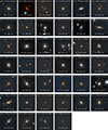 |
Fig. 5. Lens candidates in category B. The characteristics of the images are the same as in Fig. 4. |
| In the text | |
|
Fig. 6. Spectra of the five targets with source redshift estimates. The identified spectral lines are labeled, and the emission lines are indicated at the top of the image and the absorption lines at the bottom. The lines associated with the lens galaxy are shown as dashed red, and those corresponding to the source are plotted as dotted blue. |
| In the text | |
|
Fig. 7. PyAutoLens lens modelling. It informs the judgement of whether candidates are lenses. The first column shows the postage-stamp RGB cut-out image of each lens, the second column shows a clean foreground-subtracted image from the lens model multi-Gaussian expansion, the third column shows the model lensed source in the image plane, and the fourth column shows the source-plane reconstructions. The white and yellow curves represent tangential and radial critical curves and caustics. The top row shows a successful lens model fit, which traces the multiple images of the lensed source into a single region of the source plane, consistent with a strong-lens model. The remaining three rows show lens models that rule out the lensing hypothesis because they do not show evidence for multiple images or faint source galaxy emission near the centre of the candidate lens galaxy. This ruled out six candidates in total. |
| In the text | |
|
Fig. 8. Visual inspection score related to the Einstein radii and log10(S/N) of the lensed source in IE band. The colour maps represent the VI score, and the colour transition point from red to blue was set at 1.2 because this is the visual inspection score cut for candidates in category A. Red shaded areas therefore represent a region in which we can recover category A lens candidates, and blue shaded ares represent a region in which we struggle as visual inspectors to properly recognise or miss lens candidates. |
| In the text | |
|
Fig. 9. IE magnitude of the lensed source and Einstein radius distributions of the lens candidates obtained after the automatic lens modeling (black) and LENSPOP predicted population, given the redshift and velocity dispersions of our initial sample (red). |
| In the text | |
|
Fig. 10. Example of simulations following the new procedure. The 20 simulations are an example of a target in a different range of an Einstein radius and log10(S/N) in IE band. The size of each cut-out is 15″ × 15″, and they are displayed using an MTF function using the IE and YE bands. |
| In the text | |
Current usage metrics show cumulative count of Article Views (full-text article views including HTML views, PDF and ePub downloads, according to the available data) and Abstracts Views on Vision4Press platform.
Data correspond to usage on the plateform after 2015. The current usage metrics is available 48-96 hours after online publication and is updated daily on week days.
Initial download of the metrics may take a while.