| Issue |
A&A
Volume 698, June 2025
|
|
|---|---|---|
| Article Number | A53 | |
| Number of page(s) | 19 | |
| Section | Galactic structure, stellar clusters and populations | |
| DOI | https://doi.org/10.1051/0004-6361/202554176 | |
| Published online | 03 June 2025 | |
A 3D view of dwarf galaxies with Gaia and VLT/FLAMES
II. The Sextans dwarf spheroidal★
1
Kapteyn Astronomical Institute, University of Groningen,
PO Box 800,
9700AV
Groningen,
The Netherlands
2
Instituto de Astrofísica de Canarias,
Calle Vía Láctea s/n,
38206
La Laguna, Tenerife,
Spain
3
Universidad de La Laguna, Avda. Astrofísico Fco. Sánchez,
38205
La Laguna, Tenerife,
Spain
4
Leiden Observatory, Leiden University,
Einsteinweg 55,
2333
CC Leiden,
The Netherlands
5
INAF – Osservatorio di Astrofisica e Scienza dello Spazio di Bologna,
Via Gobetti 93/3,
40129
Bologna,
Italy
6
Dipartimento di Fisica e Astronomia, Università degli Studi di Firenze,
Via G. Sansone 1,
50019
Sesto Fiorentino,
Italy
7
Institute of Astronomy,
Madingley Road,
Cambridge
CB3 0HA,
UK
8
Institute of Physics, Laboratory of Astrophysics, Ecole Polytechnique Fédérale de Lausanne (EPFL),
1290
Sauverny,
Switzerland
9
European Southern Observatory,
Karl-Schwarzschild-Str. 2,
85748
Garching bei München,
Germany
★★ Corresponding author: This email address is being protected from spambots. You need JavaScript enabled to view it.
Received:
18
February
2025
Accepted:
3
April
2025
Abstract
The Sextans dwarf spheroidal galaxy has been challenging to study in a comprehensive way as it is highly extended on the sky, with an uncertain but large tidal radius of between 80–160 arcminutes (or 3–4 kpc), and an extremely low central surface brightness of ∑V ∼ 26.2 mag/arcsec2. Here, we present a new homogeneous survey of 41 VLT/FLAMES multi-fibre spectroscopic pointings that contain 2108 individual spectra, and combined with Gaia DR3 photometry and astrometry we present υlos measurements for 333 individual red giant branch stars that are consistent with membership in the Sextans dwarf spheroidal galaxy. In addition, we provide the metallicity, [Fe/H], determined from the two strongest Ca II triplet lines, for 312 of these stars. We look again at the global characteristics of Sextans, deriving a mean line-of-sight velocity of ⟨υlos⟩ = +227.1 km/s and a mean metallicity of ⟨[Fe/H]⟩ = −2.37. The metallicity distribution is clearly double-peaked, with the highest peak at [Fe/H] = −2.81 and another broader peak at [Fe/H] = −2.09. Thus, it appears that Sextans hosts two populations and the superposition leads to a radial variation in the mean metallicity, with the more metal-rich population being centrally concentrated. In addition, there is an intriguing group of nine probable members in the outer region of Sextans at higher [Fe/H] than the mean in this region. If these stars were confirmed as members, they would eliminate the metallicity gradient. We also look again at the colour–magnitude diagram of the resolved stellar population in Sextans, and at the relation between Sextans and the intriguingly nearby globular cluster, Pal 3. The global properties of Sextans have not changed significantly compared to previous studies, but they are now more precise, and the sample of known members in the outer regions is now more complete.
Key words: stars: abundances / galaxies: dwarf / galaxies: evolution / galaxies: individual: Sextans dwarf spheroidal
Based on VLT/FLAMES observations collected at the European Organisation for Astronomical Research (ESO) in the Southern Hemisphere under programmes: 171.B-0588; 60.A-9800; 0102.B-0786.
© The Authors 2025
 Open Access article, published by EDP Sciences, under the terms of the Creative Commons Attribution License (https://creativecommons.org/licenses/by/4.0), which permits unrestricted use, distribution, and reproduction in any medium, provided the original work is properly cited.
This article is published in open access under the Subscribe to Open model. This email address is being protected from spambots. You need JavaScript enabled to view it. to support open access publication.
1 Introduction
The Sextans dwarf spheroidal (dSph) galaxy is the faintest and most diffuse of the so-called classical dSphs around the Milky Way. It was found in 1990 and was one of the last Local Group galaxies to be discovered exclusively on photographic plates (Irwin et al. 1990). The Sextans dSph was also one of the first resolved galaxies to be found by an automated scanning algorithm, which picked out an enhancement of stellar point sources despite it being barely visible on the plate to the human eye. Sextans remains a difficult galaxy to display without resorting to image processing tricks. This is partly caused by its relatively low Galactic latitude (l= 243.5 b= +42.3), which results in significant contamination by foreground Milky Way disc stars. Most critically, the Sextans dSph has a very low central surface brightness (∑V ∼ 26.2 mag/arcsec2) and a large physical extent on the sky with very few member stars per arcsecond squared.
The distance to the Sextans dSph has been determined in a number of different ways making use of the stellar population in the central region. The most recent study of the variable star population (Vivas et al. 2019) has detected 199 RR Lyrae and 16 dwarf Cepheid variable stars. Of these, there are 41 RR Lyraes with complete light curve coverage, and using the period-luminosity-metallicity relation (Sesar et al. 2017), the distance is found to be 84.7 kpc. This agrees well with previous distance estimates (e.g. Irwin & Hatzidimitriou 1995; Mateo et al. 1995; Lee et al. 2009; Medina et al. 2018).
The structural properties, including the precise centre of the galaxy, have always been challenging to define as they require wide-field sensitive and uniform imaging to improve on the early photographic plate results (Irwin & Hatzidimitriou 1995). The structural parameters vary quite a bit between different studies (e.g. Irwin & Hatzidimitriou 1995; Roderick et al. 2016; Okamoto et al. 2017; Cicuéndez et al. 2018; Tokiwa et al. 2023). For example, the nominal King tidal radius has been determined with a range from 160′ ± 50 to 82′ ± 7, which means from 4 to 3 kpc at the distance of the Sextans dSph. Cicuéndez et al. (2018) provide a detailed overview of the complex situation and suggest a nominal King tidal radius of 120′. The variety of values found in the literature is due to the difficulties in treating the extremely low-surface-brightness outer regions of Sextans, where few individual stars can be unambiguously identified as members on the basis of photometry alone. Radial velocities from stellar spectroscopy and proper motions of individual stars provide uniquely valuable information to disentangle the sparse Sextans stars from those of the Milky Way, and hence to clean up our picture of the structural properties of the Sextans dSph.
A pre-Gaia ground-based proper motion study, using Subaru Suprime Cam images taken 10 years apart (Casetti-Dinescu et al. 2018), obtained a global proper motion of (μα cos δ, μδ) = (−0.409 ± 0.050, −0.047 ± 0.058) mas yr−1. This is within the errors of the Gaia eDR3 proper motion (μα cos δ, μδ) = (−0.40 ± 0.01, 0.02 ± 0.02) mas yr−1 (Battaglia et al. 2022). Numerous Gaia based determinations of the membership probabilities of individual stars in the Sextans dSph have been made, mostly to determine the dynamical motion of Sextans around the Milky Way, but also to better define its structural properties (e.g. Pace & Li 2019; McConnachie & Venn 2020; Martínez-García et al. 2021; Li et al. 2021; Pace et al. 2022; Battaglia et al. 2022; Jensen et al. 2024).
There have also been a number of low- and high-resolution spectroscopic studies of increasingly large samples of stars in the Sextans dSph (e.g. Da Costa et al. 1991; Suntzeff et al. 1993; Hargreaves et al. 1994; Kleyna et al. 2004; Walker et al. 2009; Kirby et al. 2010; Battaglia et al. 2011; Theler et al. 2020; Walker et al. 2023). These have shown that Sextans is a predominantly metal-poor (MP) galaxy. The presence or absence of cold substructures and kinematic anomalies has been debated back and forth over the years (Kleyna et al. 2004; Walker et al. 2006; Battaglia et al. 2011; Cicuéndez & Battaglia 2018; Kim et al. 2019). Several detailed chemical abundance analyses have been made, often with particular attention paid to the search for the most MP stars (e.g. Shetrone et al. 2001; Aoki et al. 2009; Tafelmeyer et al. 2010; Theler et al. 2020; Aoki et al. 2020; Mashonkina et al. 2022; Roederer et al. 2023). The scatter of the α-element abundances compared with [Fe/H] in the Sextans dSph in some of the older studies has been found to be larger than for other dSph galaxies (e.g. Aoki et al. 2009). This is maybe due to early chemical inhomogeneities, which are expected to be large in very low-mass dwarf galaxies (e.g. Roederer et al. 2023). However, more recent studies have found less scatter than the older studies (e.g. Lucchesi et al. 2020; Theler et al. 2020). This suggests that the question of the amount of abundance scatter in Sextans stars requires more study.
There have been several colour–magnitude diagram (CMD) analyses of the Sextans dSph, although these are challenging outside of the central region because of the large extent of the galaxy on the sky and the difficulties in assigning membership of individual stars to Sextans based solely on photometry. The inner regions have been well studied and there have also been impressive forays into the outer regions (e.g. Bellazzini et al. 2001; Lee et al. 2003, 2009; Okamoto et al. 2017; Cicuéndez et al. 2018; Bettinelli et al. 2019). These results are consistent with spectroscopic studies showing that Sextans has a predominantly old and MP stellar population, but there is also a more metal-rich (MR) component and there appears to be an age gradient, whereby the central regions are slightly younger than the outer regions (e.g. Okamoto et al. 2017).
As part of this VLT/FLAMES spectroscopic survey, we also include a sample of stars in the distant halo globular cluster Pal 3 due to its intriguing and well-known proximity to the Sextans dSph. This cluster was discovered well before it was realised that it was close to a low-surface-brightness galaxy (Abell 1955), and has at some points in the past been erroneously thought to be a galaxy, given its extreme isolation and distance from the Milky Way for a globular cluster. Pal 3 has previous spectroscopic measurements of radial velocities and abundance analysis (e.g. Peterson 1985; Koch et al. 2009), as well as proper motion determinations with Gaia DR3 (e.g. Vasiliev & Baumgardt 2021; Baumgardt & Vasiliev 2021), and detailed photometric studies, most precisely with the Hubble Space Telescope (Stetson et al. 1999). Its orbital properties clearly indicate an accreted origin, although its progenitor is still debated (e.g. Massari et al. 2019; Callingham et al. 2022).
This paper brings together all the available VLT/FLAMES low-resolution spectra covering the Ca II triplet (CaT) wavelength range (850–870 nm) using the LR8 grating. This provides the most extensive overview of the global properties of the resolved stellar population of this galaxy thanks to the accurate membership determination from spectroscopic radial velocities (υlos) combined with Gaia DR3 photometry and proper motion measurements.
2 The VLT/FLAMES spectroscopic observations of individual stars in the Sextans dSph
Here, we present our new measurements of υlos and [Fe/H] for new and archival data for individual stars in the Sextans dSph from the ESO (European Southern Observatory) Very Large Telescope (VLT) FLAMES/GIRAFFE spectra of red giant branch (RGB) stars. These data were collected between 2003 and 2019 in two main observing campaigns1 (see Table A.1). The LR8 grating was used; this covers the wavelength range between 8204 Å and 9400 Å at a resolving power of R∼6500. The wavelength region contains the CaT absorption lines, which are used to obtain radial velocities and determine metallicities (e.g. Armandroff & Da Costa 1991; Rutledge et al. 1997; Cole et al. 2000; Tolstoy et al. 2001; Battaglia et al. 2008; Starkenburg et al. 2010). The early observations consisted of 16 FLAMES pointings and were published by Battaglia et al. (2011). Here, we re-analyse these archival observations and combine them with new observations of 25 additional pointings, mostly from 2019. This leads to more measurements in the outer regions of the Sextans dSph (see Fig. 1). All of the measurements have been determined in a uniform way. We also analysed the reliability limits of the spectroscopic determinations of υlos and [Fe/H] as they apply to the particular challenges of the Sextans FLAMES data set.
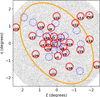 |
Fig. 1 Gaia DR3 catalogue within 3° of the centre of the Sextans dSph (grey dots), consisting of 94 770 objects that have photometry, proper motions, and parallax measurements. The horizontal and vertical axes are the local tangent plane co-ordinates corresponding to the right ascension and declination, respectively. The positions of the 41 VLT/FLAMES LR8 pointings(∼25′ diameter) are shown with dotted blue and full red circles. In blue are the 16 previously analysed fields, and in red are the 25 new fields presented here for the first time (with field IDs, as listed in Table A.1). The nominal tidal radius of Sextans from Irwin & Hatzidimitriou (1995) is shown as an orange ellipse. |
2.1 Data analysis
The Sextans dSph has some clear global differences compared to the Sculptor dSph data analysed in Tolstoy et al. (2023), hereafter Paper I. Sextans has a much lower luminosity than Sculptor and is larger on the sky, with a much lower central surface brightness (Mateo 1998), and so the number of members is a much smaller fraction of the background, and a smaller number in total, despite a similar number of pointings. The Sextans spectra have on average a higher signal-to-noise ratio (S/N) than those of Sculptor in Paper I. The systemic velocity of Sextans is about 100 km/s higher than that of Sculptor and this means that all three CaT lines lie directly under strong sky lines for Sextans stars. In Fig. 2, we show examples of the spectra of three similar luminosity RGB stars with a [Fe/H] variation from −1.5 to −3.2 and a sky spectrum to show where the sky lines fall. Each of the RGB spectra have been divided by the flux in the continuum (factor ∼200–250). For the sky spectrum, to put it on the same scale as the RGB spectra, the height of the sky lines were matched to the un-sky-subtracted but normalised spectrum of DM601, which required division by a factor of 620. All of the spectra in Fig. 2, including the sky spectrum, come from different FLAMES pointings.
We carried out the VLT/FLAMES spectroscopic analysis using the techniques described in Paper I. The first step in producing a uniform catalogue of υlos and [Fe/H] measurements for RGB stars in the Sextans dSph is to process the 41 VLT/FLAMES LR8 pointings available in the ESO archive with the most recent ESO pipeline (via the esoreflex tool, Freudling et al. 2013). This results in 2108 individual spectra, of which 989 are new. Large numbers of non-member stars (see Fig. 3) are observed due to the difficulties in separating members and non-members based purely on photometric colours, in pre-Gaia spectroscopic selections. Our initial sample of likely members includes 388 spectra that have υlos in the range 180–260 km/s. Of these, 269 have been observed once, 58 have been observed twice, and one star has been observed three times. The multiple measurements of the same star are combined to make a single averaged measurement. The total numbers of spectra and spectroscopic members per FLAMES field are given in Table A.1. We scrutinised a number of individual spectra to determine how well the pipeline was working, paying particular attention to outliers and low-S/N spectra as well as spectra with small equivalent widths (EWs) of the CaT lines.
As is described in Paper I, the ESO pipeline output spectra were sky-subtracted and then the υlos and the EWs of the CaT lines were determined using Mike Irwin’s routines. Since Paper I was published, an upgrade of the sky-subtraction routine has been carried out (Mike Irwin, private communication), which is now more robust and better at identifying and removing sky subtraction residuals and other spurious noise. This was a critical improvement for the Sextans analysis as the radial velocity of the system means that relatively strong sky lines overlap all three CaT lines. This can be seen by comparing the strong sky emission lines in the (green) sky spectrum in Fig. 2 to the weak absorption lines we are seeking to measure, especially in the low-metallicity stars found in Sextans. It can be seen that in the most MP star in Fig. 2, the blue spectrum, which is of DM272 at [Fe/H] = −3.2, the weakest CaT (unused) line has a clear sky subtraction residual that dominates the line profile. This shows that spurious residual noise from the sky subtraction poses a risk for accurate measurements of weak lines, particularly at low S/N. We noticed that with the previous version of the pipeline the sky residuals could also dominate the CaT lines and lead to inaccurate υlos and [Fe/H] measurements when the sky lines are so close to the CaT lines. Over-subtracting the sky can result in the measured υlos being shifted towards that of the sky line (which has zero velocity variation within the measurement errors). This will make the velocity dispersion tend towards zero if the effect is frequently present. These over-subtracted sky residuals can also lead to larger EWs than the actual ones, and thus appear as an artificially high [Fe/H]. In contrast, the undersubtraction of the sky can lead to emission lines at the positions of the sky lines, but these will tend to be flagged as an obvious problem with the spectrum as emission lines are not expected in RGB spectra. We carefully scrutinised a number of spectra to make sure these kinds of effects were reduced in the revised pipeline routines and that flagging spurious EW ratios and velocity differences between measurements using different techniques removed problem cases. With this new pipeline and careful flagging of problem spectra using the expected values of EWs and the repeatability of velocity measurements, the sky subtraction works well, even for low-metallicity stars within our S/N limits.
As is described in Paper I, partly to increase the accuracy of the measurements and partly as a way to check that the spectrum behaves as would be expected for an RGB star, the υlos was determined using three different methods (crosscorrelation, line fitting, and maximum likelihood) and [Fe/H] was obtained in two different ways (summing the area in the absorption lines and fitting the line) to determine the EWs of the two strongest CaT lines. These EWs were then used to determine [Fe/H] using the calibration developed by Starkenburg et al. (2010). The CaT indicator has been shown to also be robust for varying values of [Ca/H]. This was shown by comparing CaT measurements of RGB stars in Sculptor and Fornax dSph with direct high-resolution [Fe/H] and [Ca/H] measurements (Battaglia et al. 2008; Starkenburg et al. 2010). The [Fe/H] obtained from the CaT and directly from individual Fe lines matched well for a large range of [Ca/H], a better match than for [Ca/Fe]. This scaling relation has been further tested for [Fe/H] ≥ −4 (Starkenburg et al. 2013), which is an important regime for a study of Sextans.
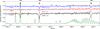 |
Fig. 2 Sky-subtracted and normalised VLT/FLAMES spectra of three RGB stars in the Sextans dSph (DM272, DM601, and DM478), with a range of [Fe/H] ∼ − 1.5 to −3.2 and υlos ∼ 230–240 km/s and all with S/N ∼ 35 per pixel. The three Ca II triplet absorption lines are easily visible in each spectrum at λλ8505 Å(EW1), 8550 Å(EW2), and 8670 Å(EW3), indicated with black arrows at top of the plot. The green sky spectrum is also normalised and plotted on the same scale. All spectra except DM601 have been arbitrarily shifted in flux to allow the spectra to be plotted together. |
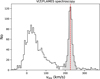 |
Fig. 3 Velocity histogram of the 2108 individual VLT/FLAMES spectra. The approximate range for members is shaded in grey (υlos = 180–260 km/s), with the expected mean velocity of members of the Sextans dSph (υlos = 227 km/s) shown as a dashed red line. |
2.2 Quality cuts
From the measured υlos from our FLAMES spectra, there are clearly many obvious Galactic foreground stars in most pre-Gaia FLAMES fields (see Fig. 3). In a few of the more recent outer fields, the Gaia pre-selection produced such a small number of targets that experiments were made to include a wider selection of targets. In addition, there are six stars in our spectroscopic sample that are likely members of the outer halo globular cluster Pal 3.
Our exploration of quality cuts for the spectra was only carried out for stars for which υlos was found to be within the broad range expected for membership. A few of these may be rejected later when we look at their properties in Gaia DR3. The S/N was determined by the pipeline from the continuum variation per pixel. There is a broad range of S/N in our measurements that does correlate with the magnitude of the star, with a degree of scatter coming from the varying conditions under which data were collected over the years. The brightest stars, G∼17, typically have a S/N∼100. At G∼18, this falls to S/N∼50 and for G > 19 mag, the maximum S/N is ∼30.
To understand the type of problems we find in our spectra of stars with υlos consistent with membership in Sextans, especially at low S/N, we looked at a number of individual spectra. We also checked measurements that ought to be well behaved for RGB stars. Thus, we investigated the difference in measuring υlos from the same spectrum in independent ways, which we call the velocity difference (vdiff) criterion. This should be small for RGB spectra, as these are the type of object that the pipeline is expecting. We also looked at the ratio of the CaT EW2/EW3 measurements that are expected for RGB stars, which we call the EW criterion. This should be fixed at an fairly constant value for RGB stars. If EW2 and EW3 are contaminated by sky residuals, or cosmic ray residuals, then these should be different in the case of each line, and so the ratio will vary. Making ‘quality cuts’ on the expected values for vdiff and EW criteria helps to remove most problems expected in the spectra above the S/N threshold. We can see from looking at the spectra that those with S/N < 10 per pixel show a lot of scatter in the results caused by noise making the CaT lines difficult to measure, most especially at low metallicity. We prefer to make a cut that does not preferentially remove low-metallicity stars, although the errors will always be higher for weaker lines as given by the error bars. In the next subsection, we carefully check that the error bars are reliable.
2.2.1 υlos quality cuts
The errors on the υlos measurements from the maximum likelihood method (MLM) over the entire survey (for S/N < 80 per pixel), plotted in Fig. 4, are well behaved. These formal errors provided by the pipeline can be compared with the velocity differences between two independent methods of measuring υlos applied to the same spectrum. This is shown in Fig. 5, in which the MLM method (vMLM) and the more straightforward cross-correlation method (vXcorr) are compared. In Fig. 5, the combined error estimates from the pipeline in Fig. 4 are given as dashed red lines. These mean lines suggest that the formal errors based on the ESO pipeline error arrays and the scatter from indivdual measurements are very similar, which means that the error determinations are reliable and well behaved down to our S/N threshold. There is a noticeable offset in the scatter in Fig. 5, in that there are more positive velocity differences than negative ones, so vMLM tends to be slightly higher than vXcorr. This is likely due to the differences in the two methods of measuring υlos. The MLM modelling has three fit parameters, an overall scale factor, a Gaussian full width at half maximum, and υlos, and makes use of the pipeline data error estimates. The X-corr method only considers υlos and ignores everything else.
Based on Figs. 4 and 5, we determined that the quality cut on the S/N of the spectra for reliable and accurate υlos measurements is S/N>10 per pixel. We also determined, from visual inspection of a selection of spectra, that stars with |vMLM − vXcorr| > 4 km/s typically have some issue with either poor sky subtraction or perhaps spurious cosmic rays, or are not RGB stars, so the stars outside our quality control selections in Figs. 4 and 5 were verified as typically being spectra with problems, usually related to not being an RGB star.
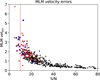 |
Fig. 4 Maximum likelihood method (MLM) velocity errors as a function of the S/N per pixel for measurements of υlos for individual VLT/FLAMES LR8 spectra of likely RGB member stars in the Sextans dSph, with G < 19.7. The blue squares are stars that do not pass the velocity quality criterion and the red stars ones that do not pass the EW quality criterion; some fail on both. The vertical dotted red line indicates the acceptable limit (S/N > 10) that is applied to the final selection of υlos measurements, bearing in mind that the blue squares and red stars were removed before the cut. |
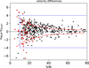 |
Fig. 5 Differences in υlos measured with the maximum likelihood (vMLM) and the cross-correlation (vXcorr) methods as a function of the S/N per pixel for the individual VLT/FLAMES LR8 spectra of likely RGB members of the Sextans dSph with G < 19.7. Red star symbols represent those stars that do not meet the EW criterion. The vertical dotted blue line shows the minimum acceptable S/N = 10, and the horizontal dotted blue lines show the limits for outliers, at ±4 km/s. The dotted black line is at vMLM − vXcorr = 0. The dashed red lines are the running mean for the combined direct error estimates made on the individual velocity measurements from the two different methods. |
2.2.2 Equivalent width quality cuts
Accurate EW measurements of the CaT lines are more exacting than υlos measurements, as EWs require a determination of the line shape as well as the peak. However, the ratios EW2/EW1 and EW2/EW3 will be around a fixed value for RGB stars. This is quantified in Fig. 6, in which we show how these ratios behave for the individual VLT/FLAMES LR8 spectra of υlos likely members. When the spread in these ratios increases for a given S/N, the measurements are less reliable because of increasing uncertainties. In the case of our spectroscopic sample, this can be a useful indicator that either the object is not an RGB star or that the CaT lines are contaminated by sky residuals, both cases making the measurement unreliable, and the object should therefore be removed from the sample. From Fig. 6, it is obvious that the scatter is less for the ratio of stronger lines (EW2/EW3) and this is why these are the only lines we use in the CaT [Fe/H] determination (e.g. Starkenburg et al. 2010) and this is also why it is also only ratio we use to select reliable spectra. This is our EW criterion. The scatter in the ratio EW2/EW3 in Fig. 6 appears well behaved for S/N ≳ 16 per pixel. Therefore, this is our threshold for a reliable [Fe/H] determination. For lower S/N, the errors become large enough to make the measurements too uncertain with a scatter that tends towards higher values of the ratio. This S/N threshold is higher than is required for accurate υlos, as was expected. This is also confirmed by looking at the [Fe/H] errors determined by the pipeline as a function of S/N per pixel (Fig. 7) and also from looking at individual spectra.
The EW2/EW3 ratio is not a perfect quality cut for our spectra, as if a spectroscopic target is not an RGB star in the Sextans dSph there can be no significant lines in the right places, and the pipeline can find similar noise at the positions of EW2 and EW3 resulting in a ratio around 1, consistent with the scatter around what is expected. Being able to tell the difference between a low-metallicity RGB star with weak lines and a different type of spectrum, meaning not a member of Sextans, often requires visual inspection to check if a spectrum is clearly an RGB spectrum, with visible CaT lines. Also, when we see clear signs of line blending in a spectrum, often leading to surprisingly high EWs, this suggests that the target is a double star (either intrinsic or by chance). Most objects like this were removed by the vdiff and EW quality cuts. One peculiar object remained (S07-80), with an unusually high [Fe/H]= +0.16. There are two spectra of this object, and both show possible signs of being two overlapping stars, one with narrow CaT lines and one with broad ones. We removed it from further consideration as a probable double spectrum.
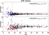 |
Fig. 6 Ratios of the EWs of the Ca II Triplet lines EW3 and EW1 with respect to the strongest line, EW2, as function of the S/N per pixel for individual VLT/FLAMES LR8 spectra that are likely members of the Sextans dSph with G < 19.7. Blue squares are spectra that do not meet the vdiff criterion. The vertical dotted red line in the upper panel is at S/N = 16 per pixel, which is the cut for accurate [Fe/H] measurements based on EW2/EW3. The horizontal dotted blue lines are limits of the values of the ratios at 0.9 < EW2/EW3 < 1.7. In the lower plot, red star symbols do not meet the limits in the upper plot for EW2/EW3. The dashed horizontal red lines in both panels show the mean of the ratios at a S/N > 40 per pixel. |
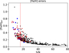 |
Fig. 7 [Fe/H] errors as a function of S/N per pixel for measurements of individual VLT/FLAMES LR8 spectra, consistent with membership in the Sextans dSph and with G < 19.7. The blue squares are stars that do not pass the vdiff criterion and the red star symbols ones that do not pass the EW criterion; some fail on both. The vertical dotted red line indicates S/N = 16 per pixel, the cut that was applied to the final selection of reliable [Fe/H] measurements. |
2.2.3 Making a final sample of FLAMES measurements
It is clear that quality cuts depend on the use that will be made of the final set of measurements. To look for interesting and unusual populations for further follow-up, it might be interesting to also consider observations at lower S/N, bearing in mind that there will be larger uncertainties. The cut for S/N > 10 per pixel provides a uniform and well-defined spectroscopic data set to determine the global stellar properties of the Sextans dSph, which is the aim of this paper. Of the original 2108 spectra, six objects are not found in Gaia DR3, and so they were removed from further analysis, as would have happened anyway, as their υlos are clearly inconsistent with them being members.
2.3 Large spectroscopic surveys with other telescopes
Several other medium-resolution spectroscopic surveys of the Sextans dSph have been made with other telescopes. The most extensive survey, with publicly available tables, is the Michigan/MIKE Fiber Spectrograph (MMFS) survey (Walker et al. 2009), recently updated and combined with a MMT/Hectochelle survey (Walker et al. 2023). This study uses the Mg-triplet spectral range (∼5150–5200 Å). It provides a huge database of measurements based on individual spectra, although many are of quite low S/N. There are 4257 Hectochelle spectra of stars in the direction of Sextans, and 2848 spectra from Magellan/M2FS, and an additional 213 M2FS spectra at medium resolution all matched to Gaia DR3. From these very large numbers, we made a selection matching our own criteria, such that G< 19.7 and 180 < υlos < 260 km/s, and we also required that the total number of observations of each source, after their quality-control filter flag had been applied good_n_obs, was greater than zero. This results in 217 stars found in both surveys and 146 stars in the Walker et al. survey and not in FLAMES.
The measurements in common between the FLAMES survey and the Walker et al. survey were used to make a comparison (see Appendix B). There are 450 spectra of reasonable quality of the 217 stars in common, and these can all be used in the comparison. From this comparison, we can see that the υlos measurements agree well. Thus, we can add the Walker υlos measurements to our kinematic sample, after first determining the calibration offset between the two surveys, as is also described in Appendix B. Adding the Walker et al. measurements of υlos for additional stars to our survey does not change our results. It fills in an area close to the centre of the Sextans dSph where FLAMES has not observed many targets and this is a region where structures have previously been found (e.g. Cicuéndez & Battaglia 2018). When we include the υlos measurements from Walker et al. in our plots, we always use distinct symbols for this sub-sample. The [Fe/H] determinations between the surveys are also compared in Appendix B, but in this case the scatter is quite large at any S/N and not symmetric around an offset value, so the [Fe/H] from Walker et al. (2023) are not included in our plots or analysis. New more complete samples will undoubtedly become available in the near future when DESI, WEAVE, 4MOST, and the Subaru Prime Focus Spectrograph survey look at the Sextans dSph.
3 Gaia DR3 aided membership determination
For individual stars, Gaia DR3 provides the parallax, proper motion in right ascension and declination, and uniquely wellcalibrated photometry. These can all be combined with our spectroscopic radial velocities to provide a robust likelihood determination of stars being members of the Sextans dSph. Combining all this different information also means that we do not need to invoke too many prior assumptions in identifying members, which allows an unbiased assessment to be made of where the limits of membership lie. The exact approach used for Sculptor in Paper I does not work for Sextans as the foreground (Galactic) contamination is much larger, the Galactic latitude is considerably lower, and the proper motions of Sextans are neither as precisely measured nor significantly different from the foreground Galactic population. This makes the inclusion of radial velocity measurements from ground-based surveys all the more important.
3.1 Bayesian approach
The exquisite photometry and astrometry from Gaia has motivated the development of Bayesian techniques that determine robust membership probabilities for individual stars in nearby dSph galaxies, making use of detailed prior information that determines the expected properties of stars in a dSph galaxy compared to other stellar populations in the same field (e.g. Pace & Li 2019; McConnachie & Venn 2020; Battaglia et al. 2022; Sestito et al. 2023). Different groups have focused on different aspects, and here we include spectroscopic radial velocities to refine the membership likelihood for a large sample of individual RGB stars found in the direction of the Sextans dSph, using the Battaglia et al. (2022) approach.
The Sextans dSph is a very low-surface-brightness system that is very large on the sky (see Fig. 8a), and thus it has always been challenging to determine its global properties. There is a lot of foreground contamination from the Milky Way and it is also not well scanned by Gaia, as can be seen in the chequered pattern in the median number of astrometric measurements per source (see Fig. 8b) and the scatter in the uncertainties in the proper motion measurements as a function of brightness (see Fig. 8c). The number of astrometric_matched_transits varies from 9 to 28, with a median of 19. For Sculptor dSph (Paper I), the number of transits went up to 60–80. The Gaia DR3 catalogue is thus slightly less deep than it was for Sculptor, going down to G = 20.85 compared to 21.20 for Sculptor (as measured by the M10 parameter, Cantat-Gaudin et al. 2023).
For Sculptor (Paper I), the stellar population of the galaxy clearly stands out in the CMD without any processing, because it is a higher-density system embedded in a lower-density Milky Way foreground. Sculptor also stands out well in parallax and proper motion plots, and thus a simple χ2 membership selection based on the astrometry worked well. For the Sextans dSph, the histogram of the Gaia DR3 calculated membership score, z (as explained in Tolstoy et al. 2023), based on proper motion and distance measures and their errors, shows no structure that makes clear where a membership cut should be made. A selection for z < 14.2 does bring out the CMD of Sextans more clearly. However, there remains a lot of Milky Way contamination. Thus, we should also take into account the spatial and CMD distribution of the stars in the field to improve the selection of the likely Sextans members. This has already been done with a mixture model in Battaglia et al. (2022), and so we used their methodology to update their membership probabilities on the wider area covered by our spectroscopic survey and using the υlos spectroscopic information where possible (see Sect. 4.2.1 of their article).
From the Gaia DR3 catalogue, we extracted all the sources with three-colour photometry and astrometry (parallax and proper motions) within a circle of radius 3 degrees around the central position of the Sextans dSph (Irwin & Hatzidimitriou 1995, see Fig. 8a), which is 94 770 sources. By far the majority of these sources are not members of Sextans, and they have a membership probability of Pmem = 0 in Battaglia et al. (2022).
Gaia DR3 information alone already presents an excellent probability of membership (Pmem). The inclusion of the FLAMES υlos information results in a more precise identification of highly likely members and obvious non-members and of course provides more information about each star.
We looked for a value of Pmem below which our spectra were mostly clearly velocity non-members, and above mostly velocity members. This leads to a cut for likely membership whereby Pmem > 0.07 for stars with G < 19.7. This leaves 604 likely members based on Gaia DR3 probabilities alone. The magnitude limit, G < 19.7, was applied because the Gaia astrometry is less reliable for the fainter stars and this is also the case for the υlos measurements from FLAMES, and so the membership probabilities are less reliable for fainter stars.
A FLAMES υlos consistent with membership in the Sextans dSph is available for 333 Gaia DR3 member stars, with S/N > 10 per pixel. This is a little over half the likely members (604) found using only the Gaia DR3 information for stars with G < 19.7. The rest of the Gaia DR3 likely members are not in our FLAMES sample. These are all in the expected range of ±5σ around the mean of the υlos, showing the power of Gaia proper motions for membership selection. In addition, there are nine stars that have Pmem = 0, but υlos in the expected range of membership. Looking at these stars more carefully, we see that they are at the edge of several selection criteria for Gaia DR3 membership and they were removed because of this. They all have good RUWE values and a good number of visibility periods, and only three of the stars have an elevated crowding (pd_gof_harmonic_amplitude ≳ 0.1), but these are the ones closest to the centre of Sextans. So there is no strong indication (also from looking at the spectra) that these stars are binary stars. Thus, it is plausible that they could be members and they are retained as possible members, and plotted with different symbols in all future plots.
An overview of the global picture from Gaia DR3 is displayed in Fig. 9, where we show the collective distribution of the different properties we can measure for the resolved stellar population of Sextans dSph. We identify the different samples with different symbols in all plots.
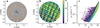 |
Fig. 8 Gaia DR3 data within 3 degrees of the centre of the Sextans dSph. (a) Distribution of sources on the sky; (b) Median number of astrometric observations (astrometric_matched_transits) matched to a given source; (c) Uncertainty on μδ as a function of G. The orange ellipse in panels a and b indicates the nominal tidal radius of the Sextans dSph. |
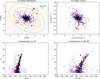 |
Fig. 9 Gaia DR3/FLAMES membership selection for the Sextans dSph: (a) spatial distribution of Gaia DR3 positions overlaid with the spectroscopic members. The largest solid orange ellipse is the nominal tidal radius from Irwin & Hatzidimitriou (1995). The dashed line ellipses are from Cicuéndez et al. (2018) (outer) and Roderick et al. (2016) (inner). The black arrow is the mean proper motion on the sky of Sextans and the green arrow is the same for the Pal 3 globular cluster, which is at the position of the green ellipse; (b) Gaia DR3 proper motions in RA and Dec; (c, d) CMDS from Gaia DR3 photometry. In all plots, grey dots are the Gaia DR3 catalogue entries, for G < 19.7. The magenta dots are the 604 likely members of Sextans (Pmem > 0.07). Overplotted as black dots are 333 Gaia/FLAMES members (with S/N > 10 per pixel and G < 19.7) and 146 blue dots from Walker et al. (2023) that are not in the FLAMES catalogue. The nine red stars are in the FLAMES sample with a υlos consistent with membership, but just outside the Gaia membership criteria. The three red stars with an additional black circle have lower υlos than the rest of the member stars (υlos < 190 km/s), but ones that are still within 4σ of the mean systemic υlos. |
3.2 Completeness of the Gaia DR3-LR8 survey
Fig. 9a shows very few stars outside the nominal tidal radius of the Sextans dSph defined by Irwin & Hatzidimitriou (1995). It also shows that there is a (small) hole in the spatial coverage of FLAMES measurements (black dots) in the central region. There are velocity measurements from Walker at this position (blue circles) instead. They do not significantly change the analysis, but they are identified in the plots as the scatter is often quite large.
In Fig. 10, we show the overall completeness of the spectroscopic follow-up in the Sextans dSph. The Gaia DR3 selection function (Cantat-Gaudin et al. 2023) shows that in the sky area of Sextans Gaia DR3 is complete to G = 20. In Fig. 10a, we show the fraction of the complete sample of Gaia DR3 likely members that have FLAMES spectroscopic follow-up. Adding in the Walker et al. sample gives close to 90% completeness for the spectroscopic follow-up of stars with G < 18.5. It can be seen that the total number of stars rapidly increases with decreasing G in Fig. 10b, and the completeness with distance from the centre of the galaxy is decreasing, in Fig. 10c, although the total number of stars also decreases rapidly from the centre of the galaxy. The spatial distribution of the Gaia DR3 members can be seen in Fig. 9a. The improved completeness in the outer regions comes from a relatively small number of stars and despite the effort that it takes to find them, they are important for understanding the true extent of the system and its properties and we have provided a more complete picture of Sextans than was previously available.
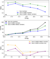 |
Fig. 10 Completeness of the VLT/FLAMES LR8 survey relative to the complete Gaia DR3 members (G < 19.7 and Pmem > 0.07) for the Sextans dSph as a function of Gaia DR3 G magnitude and Elliptical radius (rell), including the increased completeness from adding in Walker et al. (2023) υlos measurements: (a) as a fraction of the total Gaia DR3 members (black), those with FLAMES confirming spectra (blue), and those with FLAMES plus Walker23 (green); (b) the total number of stars, with measurements from Gaia DR3 (black), Gaia DR3+FLAMES (blue), and Gaia DR3+FLAMES+Walker (green); (c) the completeness as a function of rell, for Gaia DR3+FLAMES (purple) and Gaia DR3+FLAMES+Walker (orange), with a dotted black line at 50% completeness. |
4 Results
From the data analysis and quality criterion cuts in the previous section, we have a catalogue of 604 likely members of the Sextans dSph based on Gaia DR3, and of these 325 have supporting υlos measurements of acceptable quality from our FLAMES spectroscopic sample. There are an additional nine probable members based on their spectroscopic υlos and borderline non-member Gaia parameters. We included these additional stars in our plots as distinct symbols, and they are not included in global averages or analyses. Of these, 312 also have [Fe/H] measurements of acceptable quality, which includes these nine probable members. An additional 146 of our 604 Gaia DR3 members have υlos measurements from Walker et al. (2023); these are included in the plots with different symbols. This makes a total of 480 stars with υlos spectroscopic measurements as well as Gaia astrometry consistent with membership.
The full sample of measurements of the 604 likely members of the Sextans dSph is presented online (Table D.1). Table D.1 includes, where it is available, FLAMES spectroscopic information, and for those stars not in the FLAMES sample but that have a reliable Walker υlos measurement (Walker et al. 2023), Walker υlos measurements are also included in Table D.1. In addition, the FLAMES spectroscopic and Gaia DR3 properties of the nine probable members that are υlos members but that have uncertain Sextans membership based on Gaia DR3 are included in Table D.1.
In Table D.2, we also provide the Gaia DR3 and spectroscopic information for the stars for which we have FLAMES observations but that are either very clear non-members on the basis of their spectroscopic υlos or that do not have reliable enough spectroscopic measurements. If the unreliable spectroscopic members are likely Gaia members then this also noted in Tables D.1 and D.2.
For the Gaia/FLAMES sample with Pmem > 0.07 (so excluding the nine stars with borderline Gaia parameters), combined with a υlos consistent with membership, the mean FLAMES spectrosopic and astrometric parameters for the entire Sextans dSph galaxy are given in Table 1. These agree with previous determinations, with the exception of the mean metallicity, ⟨[Fe/H]⟩, which has become significantly lower, due to the complex metallicity distribution function (MDF) of Sextans with a metallicity gradient declining in the outer parts, making a mean metallicity highly dependent on the size and spatial distribution of a sample. The differences in the astrometric parameters with the full Gaia DR3 sample (given by Battaglia et al. 2022) are within the uncertainties.
In Fig. 11, we show the spatial distribution of the Gaia DR3/FLAMES measurements for the central region of Sextans colour-coded by [Fe/H] in Fig. 11a and by υlos in Fig. 11b. There do appear to be some clumps in the spatial distribution, but this is a common effect of small number statistics and there is nothing that stands out as having a single metallicity or a single υlos. There are structures in the spatial distribution of likely members in Fig. 11, but they always contain a range of [Fe/H] and υlos values so that nothing stands out as different from the overall population. Evidence has been presented for sub-structures that do show coherent properties in υlos and relative metallicity in the central region of Sextans (e.g. mostly recently by Cicuéndez & Battaglia 2018) but we miss a large fraction of the region used in this work. This is the ‘hole’ near the centre of Sextans for which there are measurements from the Walker et al. (2009) survey that was used by Cicuéndez & Battaglia (2018).
Mean properties of the Sextans dSph.
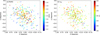 |
Fig. 11 Spatial distribution of the Gaia DR3/FLAMES members across the Sextans dSph: a) coloured by [Fe/H]; b) coloured by υlos. The grey dots are the Gaia DR3 likely members without FLAMES spectra. |
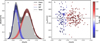 |
Fig. 12 Properties of the sample of spectroscopically observed member stars of the Sextans dSph, not including the nine probable members, with reliable [Fe/H] information. Panel a: normalized [Fe/H] distribution with the best-fitting two-population model. The dashed lines indicate the predicted distribution of our model: red for the MR component, blue for the MP, and black for the sum of the two components as indicated in the legend. Bands indicate the 1σ confidence intervals. Panel b: projection of the stars in the υlos vs [Fe/H] plane; the systemic velocity of Sextans is indicated with the horizontal line. The velocities have been corrected for the reflex motion between the Sun and Sextans. |
4.1 The VLT/FLAMES spectroscopic metallicities
In Fig. 12a, we show the histogram distribution of the FLAMES [Fe/H] measurements, with S/N > 16 per pixel and G < 19.7 for RGB stars in the Sextans dSph. It clearly has a a doublepeaked MDF, with a MR and MP peak. The comparison of the kinematic properties of the MR and the MP population is shown in Fig. 12b, in which it can be seen that the MP population has a higher velocity dispersion than the MR (see also Table 2). The colour code in Fig. 12b shows the probability of a star belonging to the MR population, showing the clear distinction between the bulk of the two populations.
In Fig. 13, we show the distribution of the FLAMES [Fe/H] measurements as a function of elliptical radius (rell), showing a clear decline in the mean [Fe/H] with increasing distance from the centre of the galaxy, albeit with a large scatter. The nine stars with borderline Gaia DR3 membership properties present an intriguing subset. Of this sample, six are at rell > 1.5 deg from the centre. There are only eight other members in this extremely low-surface-brightness outer region of this galaxy. It is difficult to interpret the fact that the mean [Fe/H] of these six outer probable-member stars are clearly ≳1 dex more MR than all the other eight stars in these outer regions. There is no particular distinction in the spatial distribution of these probable members (see Fig. 9). It would be easy to interpret this as a sign that these stars must be non-members, but we think that the question must be left open for now. There are three additional stars with borderline Gaia membership at around rell ≈ 0.5 deg; they are more MP than the outer six, and they fit in well with the rest of the stars found around this distance from the centre of the galaxy. These three are clearly less contentious, but this shows the risks of deciding membership too strongly on the basis of expectations for the results. For now, this must remain an unsolved conundrum.
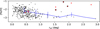 |
Fig. 13 [Fe/H] for stars plotted with elliptical radius, rell, which is the projected semi-major axis radius, as black circles for the 312 measurements with S/N > 16 per pixel in our Sextans dSph sample. The blue line shows the binned mean and the error bars are the dispersion in each bin for the black points. The red star symbols are the nine possible members of Sextans not included in the blue mean determination, with the three with unusually low υlos circles in black. |
Global properties of the Sextans dSph.
4.2 Global kinematic properties
In order to quantify the presence or absence of a line of sight (l.o.s.) velocity gradient, we followed the approach of Taibi et al. (2018) and compared two different models: one exclusively supported by velocity dispersion and one allowing for the presence of a deviation from the systemic velocity that is a linear function of the distance from the Galactic centre. We first corrected the l.o.s. velocities for the relative motion between the Sextans dSph and the Sun, removing perspective l.o.s. velocity gradients. If we consider only the VLT/FLAMES data set, we obtain a systemic velocity of 227.0 ± 0.5 km s−1 and a l.o.s. velocity dispersion of  in both models. The l.o.s. velocity gradient is consistent with zero within little more than 1-σ
  , and given that in our Bayesian analysis the model without rotation is moderately favoured with respect to that with rotation (by 2.1 points, using the Jeffrey scale), we conclude that there is no evidence of a l.o.s. velocity gradient in this new VLT/FLAMES data set. The results do not change if we consider the VLT/FLAMES data with the addition of the Walker et al. (2023) measurements (the l.o.s. velocity gradient in this case is 2.2 ± 1.3 km/s/deg, fully consistent with the previous value).
There is no sign of any structure in the υlos corrected for the Galactic standard of rest plotted against position along the major axis and as a function of elliptical radius (rell) in Fig. 14. The number of stars in the outer regions is relatively small, so it is hard to be conclusive about how or if the properties change towards the outer regions. The six outer probable members (plotted as red stars in Fig. 14) look a better match to the more certain measurements than is seen in Fig. 13, except for the three stars that have unusually low υlos, which are red stars circled in black in Fig. 13. If these six stars are ignored then the velocity dispersion appears to be quite a bit lower in the outer regions compared to the central regions. This is less clear if the probable members are included, but in either case the numbers are very small.
There are known to be intriguing features in the spatial distribution of kinematic data that have recently been explored (e.g. Roderick et al. 2016; Cicuéndez & Battaglia 2018). For example, Cicuéndez & Battaglia (2018) found kinematic anomalies in the Sextans dSph, in the form of a ‘ring-like’ feature exhibiting a larger mean velocity and lower relative metallicity than the control sample. This feature was found only in the spectroscopic data set of Walker et al. (2009) because the spatial coverage of the other large spectroscopic surveys existing at the time (Kirby et al. 2010; Battaglia et al. 2011) did not sufficiently cover the region where the feature is more evident. As the new data set presented here does not add significant coverage in the region of the ‘ring’ we could only verify that the velocity map obtained by performing a similar analysis to that in Cicuéndez & Battaglia (2018) appears compatible with the presence of the kinematic feature in this data set, but it does not add significant information to refine its properties.
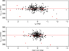 |
Fig. 14 VLT/FLAMES LR υlos for individual members in the Sextans dSph, corrected for the shift created by the motion of the Sun around the Galactic centre at the position of Sextans, rell (above); and the position along the major axis (below). The nine probable members are shown as red stars. The mean-corrected υlos is a dotted line at 342.4 km/s. |
4.3 Chemo-kinematic properties
It has already been established that the stellar component of several classical dSph galaxies around the Milky Way, including the Sextans dSph, can be described as the superposition of at least two stellar populations with different spatial distributions, mean metallicities, and kinematics (e.g. Tolstoy et al. 2004; Battaglia et al. 2006, 2008; Walker & Peñarrubia 2011; Pace et al. 2020).
The presence of multiple chemo-kinematic components in the Sextans dSph was first explored in Battaglia et al. (2011). Guided by the presence of a clear spatial variation in the metallicity properties and by the fact that the MDF could be well fitted by the sum of two Gaussians crossing at [Fe/H] ∼ − 2.3, the authors separated the sample into stars more MR than [Fe/H] = −2.2 and more MP than [Fe/H] = −2.4. They found that the υlos dispersion profile of the MR population tended to be around 6 km s−1 and slightly declining as a function of radius, while for the MP population it was approximately flat around ∼9.5 km s−1 (apart from an inner cold point, with a velocity dispersion of ∼1.4±1.2 km s−1, discussed later).
Here, we revisit the presence of multiple components using the same methodology that Arroyo-Polonio et al. (2024) have recently applied to the Sculptor dSph, broadly based on Walker & Peñarrubia (2011); Taibi et al. (2018); Pace et al. (2020). Here, we simply investigate whether the combined information about the position, [Fe/H] and υlos of member stars is best described by one population displaying a (linear) metallicity gradient or by the sum of two populations. In all cases, the surface density profile of the overall or individual stellar components is assumed to follow a Plummer profile, while the l.o.s. velocity distribution is assumed to be Gaussian. This analysis was applied to the combined sample of 303 stars selected to have S/N > 16 per pixel, G < 19.7, and a Gaia+spec probability of membership of >0.07. We corrected the l.o.s. velocities for the relative motion between the Sextans dSph and the Sun.
The Bayesian parameter estimation for each model was obtained with pymultinest. We find that the two-population model is strongly favoured, by 11 on the Jeffrey scale, over the single population model.
The main properties of the two stellar components are summarized in Table 2. Similar to previous findings and the general characteristics of multiple chemo-kinematic components in other Milky Way dSphs, the MR population is found to have a more concentrated spatial distribution and a colder velocity dispersion than the MP component (see Fig. 12). In a separate contribution, we shall analyse in detail the velocity dispersion profiles of the MR and MP population and the shape of the overall l.o.s. velocity distribution. At present, we do not see evidence of the inner cold-kinematic point found by Battaglia et al. (2011) in the l.o.s. velocity dispersion profile in this new data set.
4.4 Gaia DR3 colour–magnitude diagram
In Fig. 15, we plot the de-reddened Gaia DR3 photometry for the RGB stars that are Gaia DR3 (Pmem > 0.07) members, assuming E(B-V) ∼0.04 (Cicuéndez et al. 2018)), and where available FLAMES [Fe/H] measurements, colour-coded from MR (red) to MP (blue) as is shown on the colour bar in the plot. As in Paper I for the Sculptor dSph, we can see that the more MR stars are nicely aligned on the red side of the RGB and the more MP stars on the blue side. Towards the tip of the RGB (G < 18), there appear to be two distinct sequences. This is consistent with what has been found in Paper I, and suggests that when identifications can be made precisely enough to identify two populations in the [Fe/H] histogram and kinematically in the velocity dispersion measures then they can also be identified in their colours on the RGB of the CMD. For fainter magnitudes (G > 18.5), it is not necessarily the case that the populations are more mixed, but that the errors in all the different measurements (Gaia DR3 photometry and [Fe/H]) are increasing.
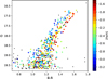 |
Fig. 15 Gaia DR3 reddening corrected CMD for the FLAMES Sextans dSph sample, with circles for those stars with reliable FLAMES Ca II triplet [Fe/H] measurements, colour-coded by [Fe/H] as is shown by the colour bar. The Gaia DR3 sample without FLAMES spectra are shown as small black points. |
4.5 Palomar 3
The Palomar 3 globular cluster was discovered long before the Sextans dSph, by A.G. Wilson in 1952, using photographic plates taken with the 48-inch Schmidt telescope at Palomar Observatory (Abell 1955). The first detailed study of the resolved stellar population was made by Burbidge & Sandage (1958), based on photographic plates from the 200-inch Hale telescope. They determined a distance of 100 kpc, very much in line with the modern determination of 95 kpc (Baumgardt & Vasiliev 2021). Palomar 3 has thus long been known to be one of the most distant globular clusters associated with the Milky Way. It is also one of a small number of Galactic globular clusters with ‘high-energy’ dynamical properties (e.g. Massari et al. 2019), so its origin and association with any known structure in the Milky Way is unknown. According to Vasiliev & Baumgardt (2021), Palomar 3 could be associated with Sagittarius debris, but the models are unreliable at these distances due to the lack of observational data. It is clearly a MP, with [Fe/H] = −1.6 dex (Ortolani & Gratton 1989; Armandroff et al. 1992; Koch et al. 2009), and a relatively old system, although probably 1.5–2 Gyr younger than the classical globular clusters (Stetson et al. 1999, see Table 3 for an overview).
It appears noteworthy that the Sextans dSph and the Palomar 3 globular cluster, both of unknown origin, lie so close on the sky, and also at such similar distances, with Palomar 3 being ∼10 kpc more distant. Their υlos are quite different, with Palomar 3 having a υlos = +92 km/s (Peterson 1985; Koch et al. 2009), and so their motion in the sky also differs markedly (see Fig. 9). Likely members of Palomar 3 have the same proper motion and parallax signatures to Sextans (very close to zero), and so they were picked up naturally in our original target selection. We observed six stars likely associated with Palomar 3 and also a selection in the region around (see Table 4 for details of the six RGB stars we observed).
The differences of the proper motion directions of the Palomar 3 globular cluster and the Sextans dSph on the sky (Fig. 9) suggest that these two systems have no relation to each other (as has long been assumed given their very different υlos). The differences in 3D motions also makes it difficult for the Palomar 3 globular cluster to be bound to the Sextans dSph, unless Sextans is much more massive than it currently appears.
We carried out a straightforward orbit integration of the two systems based on their systemic proper motions, for a potential that includes the LMC potential described in Vasiliev et al. (2021). In Fig. 16, we show how the distance between the Sextans dSph and Pal 3 changes with time. In Fig. C.1, we show the details of the orbit integrations that went into this plot. It is clear that the uncertainties grow going further back in time, but given the assumptions we have used there is no evidence that Pal 3 and Sextans have any connection or signs of past interactions. It appears that they are currently closer than they have ever been. The inferred apocentre and pericentre variations over the last 6 Gyr for Pal 3 and Sextans do overlap in Galactocentric distance but they follow different paths, with Sextans typically inhabiting more distant regions of the Milky Way halo with with a slower orbital trajectory.
If these systems have been disrupted in some way in the recent past, which could perhaps explain the extremely low surface brightness of Sextans, then of course it is more difficult to be definitive about their orbital histories and a possible relation between these two systems. However, there is no obvious cause for any disruption, so any assumption that Sextans and/or Palomar 3 are out of equilibrium would be highly speculative. We also looked for any sign of Pal 3 stars more distant from the cluster in our FLAMES sample, based on the expected υlos and proper motions, but did not find any. The proper motion errors on Pal 3 are quite large, and the true mass of Sextans, let alone the Milky Way, is quite uncertain, as is how they may have changed in the past, so there is potential for more detailed modelling, but this is well beyond the scope of this work.
Mean properties of Palomar 3.
Individual stars observed in Palomar 3.
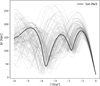 |
Fig. 16 Distance between Sextans and Pal3 going back in time, from orbit integration for both Sextans dSph and Pal 3, using the Vasiliev et al. (2021) potential. |
5 Conclusions
From a combination of new and old re-processed archival VLT/FLAMES LR8 data, we have obtained a uniform sample of [Fe/H], υlos, and Gaia DR3 astrometric parameters for 312 individual member RGB stars, extending to (and beyond) the nominal tidal radius. This has allowed us to look again at the chemo-dynamical properties of the Sextans dSph. The main difference with previous results is that given the new more uniformly distributed, and more precisely defined ‘cleaner’ sample, the scatter is much better quantified and the features suggested seen in smaller data sets are typically less compelling, but still worth more detailed investigation and modelling. We confirm that the Sextans dSph has complex υlos and [Fe/H] distributions. The MR component is clearly concentrated in the centre of the galaxy. There are kinematic and [Fe/H] sub-structures in Sextans but the sparsity of the tracers makes it difficult to know how robust they are without more detailed modelling. The wealth of information coming from the combination of spectroscopic metallicities from FLAMES and the exquisite Gaia DR3 photometry of the sample of RGB stars in the Sextans dSph suggests a complex history. Larger samples of more precise highspectral-resolution abundances would be beneficial to clarify the chemical differences in a more detailed and quantitative way.
Data availability
Full Tables D.1 and D.2 are available at the CDS via anonymous ftp to cdsarc.cds.unistra.fr (130.79.128.5) or via https://cdsarc.cds.unistra.fr/viz-bin/cat/J/A+A/698/A53
Acknowledgements
This work has made use of data from the European Space Agency (ESA) mission Gaia (https://www.cosmos.esa.int/gaia), processed by the Gaia Data Processing and Analysis Consortium (DPAC, https://www.cosmos.esa.int/web/gaia/dpac/consortium). Funding for the DPAC has been provided by national institutions, in particular the institutions participating in the Gaia Multilateral Agreement.
Appendix A The observations: Individual VLT/FLAMES pointings
In Table A.1 we list each individual FLAMES pointing. We provide the date of the observation, the ESO programme ID and the name we gave to each field as well as the RA and Dec of centre of the field, and the airmass (airm) and seeing monitor (DIMM) values. The exposure time (exp) is given. Also provided are the number of spectra in each pointing (spec) and the number of these that have a υlos expected for membership in Sextans (vmem) and also the shift in the velocity of the entire field (vshift) with respect to our zero point. This shift ensures that all our observations are on the same velocity scale and that small effects between different observations are taken into account.
LR8 observations of RGB stars in the Sextans dSph with VLT/FLAMES/GIRAFFE.
Appendix B Comparing FLAMES measurements with Walker et al. (2023)
Our FLAMES sky coverage has a hole in the central region, and thus we explore combining our observations with the study of Walker et al. (2023), where many of these measurements were already presented in Walker et al. (2009). To make sure these observations over a different wavelength region made with different telescopes can be combined with our FLAMES observations we compare the υlos and [Fe/H] of those stars that are observed in both surveys. This is shown in Fig. B.1. We matched the Walker et al. catalogue of velocities and metallicities our final set of FLAMES members using the Gaia DR3 ID. There are 442 matching measurements.
The S/N for the Walker measurements are not calculated in the same way as ours. There can be many reasons for this which we do not go into, but simply present the comparison between measurements made of the same stars and make our cuts based on this.
The differences between the Walker et al. υlos measurements and ours for the same stars in Fig. B.1 look very stable, very comparable. There is a small offset with the mean velocities measured by Walker et al. of +1.7km/s, as shown by the dotted line in the upper panel of Fig. B.1. This likely comes from using a slightly different zero point calibration. The Walker et al. velocities were set to match the APOGEE DR17 results for the same stars, so this is an offset between our measurements and APOGEE. Some stars have quite large υlos differences and these are potentially binary stars, where υlos may differ significantly over the time between measurements, but the fact most of these offset measurements tend to have a low S/N suggests this is caused simply by measurement uncertainties. The [Fe/H] measured by Walker et al. is determined using a different method to ours, namely fitting a model from a library of synthetic template spectra to the observed spectrum, providing both [Fe/H] and [Mg/Fe] determinations. Unfortunately, the resulting measurements [Fe/H] do not agree very well with ours. This is clearly seen in the lower panel of Fig. B.1, where there is a considerable scatter, that is not uniform about a mean, especially at low S/N. The offset in the mean of the high S/N measurements is +0.22dex. We have not investigated this further, we have just opted not to include these measurements in our analysis.
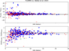 |
Fig. B.1 Comparison between Walker et al. (2023) MMT/Hectochelle and Magellan/M2FS spectroscopic results and our VLT/FLAMES results for the stars covered by both surveys. We compare with our final sample of members (G< 19.7mag, S/N> 10 per pixel). In the upper panel, we plot the υlos comparison of the two surveys and in the lower panel, [Fe/H]. The blue solid points are from the MMT and the red points are from the main M2FS survey. The green stars come from the medium resolution M2FS sample. The dashed lines are at zero and the dotted lines are the mean offset between the two surveys, (vWalker + 1.7 km/s and [Fe/H]Walker + 0.22 dex. |
Appendix C Orbit analysis of Sextans dSph and Pal 3
In Fig. C.1, we show the orbital evolution of Sextans and Palomar 3 integrating backwards in time for 6 Gyr assuming the MW potential introduced in Vasiliev et al. (2021). This is a time-dependent potential that takes into account the passage of the LMC, with mass 1.5 × 10¹¹ M⊙ that entered the MW dark matter halo about 1.6 Gyr ago, and the acceleration induced by the reflex motion of the MW. We used the code Agama (Vasiliev 2019) to perform the orbit integration. Orbital uncertainties were estimated from 100 Monte Carlo realisations by sampling the position-velocity vector of the inspected systems (shown for clarity only in the first panel of the figure).
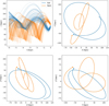 |
Fig. C.1 Details of the orbit analysis of Sextans and Pal 3. In the top left panel is the variation of the Galactocentric distance as a function of the look-back time for the two systems. In the other three panels is the orbital evolution in each of the planes of the xyz-space in Galactocentric co-ordinates. |
Appendix D The results
Here we show an example of what is available as an online table at CDS for the combined Gaia DR3 photometry and astrometry and VLT/FLAMES LR8 spectroscopy for stars in and around the Sextans dSph. In Table D.1 we show the full VLT/FLAMES LR8 plus Gaia DR3 sample of members. In Table D.2 we provide the VLT/FLAMES LR8 velocity non-members for completeness, including only the measured velocities and their Gaia DR3 IDs.
Gaia DR3 & VLT/FLAMES results for stars that are members of the Sextans dSph.
The stars in Table D.1 with Pmem=0 are stars with VLT/FLAMES spectroscopic υlos compatible with membership in Sextans but the Gaia proper motions and/or parallaxes are just on the wrong side of the membership cuts. They are borderline members.
VLT/FLAMES rejected spectra and non-members of the Sextans dSph.
References
- Abell, G. O. 1955, PASP, 67, 258 [NASA ADS] [CrossRef] [Google Scholar]
- Aoki, W., Arimoto, N., Sadakane, K., et al. 2009, A&A, 502, 569 [NASA ADS] [CrossRef] [EDP Sciences] [Google Scholar]
- Aoki, M., Aoki, W., & François, P. 2020, A&A, 636, A111 [NASA ADS] [CrossRef] [EDP Sciences] [Google Scholar]
- Armandroff, T. E., & Da Costa, G. S. 1991, AJ, 101, 1329 [Google Scholar]
- Armandroff, T. E., Da Costa, G. S., & Zinn, R. 1992, AJ, 104, 164 [Google Scholar]
- Arroyo-Polonio, J. M., Battaglia, G., Thomas, G. F., et al. 2024, A&A, 692, A195 [NASA ADS] [CrossRef] [EDP Sciences] [Google Scholar]
- Battaglia, G., Tolstoy, E., Helmi, A., et al. 2006, A&A, 459, 423 [NASA ADS] [CrossRef] [EDP Sciences] [Google Scholar]
- Battaglia, G., Irwin, M., Tolstoy, E., et al. 2008, MNRAS, 383, 183 [NASA ADS] [CrossRef] [MathSciNet] [Google Scholar]
- Battaglia, G., Tolstoy, E., Helmi, A., et al. 2011, MNRAS, 411, 1013 [NASA ADS] [CrossRef] [Google Scholar]
- Battaglia, G., Taibi, S., Thomas, G. F., & Fritz, T. K. 2022, A&A, 657, A54 [NASA ADS] [CrossRef] [EDP Sciences] [Google Scholar]
- Baumgardt, H., & Vasiliev, E. 2021, MNRAS, 505, 5957 [NASA ADS] [CrossRef] [Google Scholar]
- Bellazzini, M., Ferraro, F. R., & Pancino, E. 2001, MNRAS, 327, L15 [NASA ADS] [CrossRef] [Google Scholar]
- Bettinelli, M., Hidalgo, S. L., Cassisi, S., et al. 2019, MNRAS, 487, 5862 [NASA ADS] [CrossRef] [Google Scholar]
- Burbidge, E. M., & Sandage, A. 1958, ApJ, 127, 527 [Google Scholar]
- Callingham, T. M., Cautun, M., Deason, A. J., et al. 2022, MNRAS, 513, 4107 [NASA ADS] [CrossRef] [Google Scholar]
- Casetti-Dinescu, D. I., Girard, T. M., & Schriefer, M. 2018, MNRAS, 473, 4064 [NASA ADS] [CrossRef] [Google Scholar]
- Cantat-Gaudin, T., Fouesneau, M., Rix, H.-W., et al. 2023, A&A, 669, A55 [NASA ADS] [CrossRef] [EDP Sciences] [Google Scholar]
- Cicuéndez, L., & Battaglia, G. 2018, MNRAS, 480, 251 [CrossRef] [Google Scholar]
- Cicuéndez, L., Battaglia, G., Irwin, M., et al. 2018, A&A, 609, A53 [NASA ADS] [CrossRef] [EDP Sciences] [Google Scholar]
- Cole, A. A., Smecker-Hane, T. A., & Gallagher, III, J. S. 2000, AJ, 120, 1808 [Google Scholar]
- Da Costa, G. S., Hatzidimitriou, D., Irwin, M. J., & McMahon, R. G. 1991, MNRAS, 249, 473 [Google Scholar]
- Freudling, W., Romaniello, M., Bramich, D. M., et al. 2013, A&A, 559, A96 [NASA ADS] [CrossRef] [EDP Sciences] [Google Scholar]
- Gaia Collaboration (Helmi, A., et al.) 2018, A&A, 616, A12 [NASA ADS] [CrossRef] [EDP Sciences] [Google Scholar]
- Hargreaves, J. C., Gilmore, G., Irwin, M. J., & Carter, D. 1994, MNRAS, 269, 957 [NASA ADS] [CrossRef] [Google Scholar]
- Irwin, M., & Hatzidimitriou, D. 1995, MNRAS, 277, 1354 [NASA ADS] [CrossRef] [Google Scholar]
- Irwin, M. J., Bunclark, P. S., Bridgeland, M. T., & McMahon, R. G. 1990, MNRAS, 244, 16 [NASA ADS] [Google Scholar]
- Jensen, J., Hayes, C. R., Sestito, F., et al. 2024, MNRAS, 527, 4209 [Google Scholar]
- Kim, H.-S., Han, S.-I., Joo, S.-J., Jeong, H., & Yoon, S.-J. 2019, ApJ, 870, L8 [NASA ADS] [CrossRef] [Google Scholar]
- Kirby, E. N., Guhathakurta, P., Simon, J. D., et al. 2010, ApJS, 191, 352 [NASA ADS] [CrossRef] [Google Scholar]
- Kleyna, J. T., Wilkinson, M. I., Evans, N. W., & Gilmore, G. 2004, MNRAS, 354, L66 [Google Scholar]
- Koch, A., Côté, P., & McWilliam, A. 2009, A&A, 506, 729 [NASA ADS] [CrossRef] [EDP Sciences] [Google Scholar]
- Lee, M. G., Park, H. S., Park, J.-H., et al. 2003, AJ, 126, 2840 [NASA ADS] [CrossRef] [Google Scholar]
- Lee, M. G., Yuk, I.-S., Park, H. S., Harris, J., & Zaritsky, D. 2009, ApJ, 703, 692 [NASA ADS] [CrossRef] [Google Scholar]
- Li, H., Hammer, F., Babusiaux, C., et al. 2021, ApJ, 916, 8 [CrossRef] [Google Scholar]
- Lucchesi, R., Lardo, C., Primas, F., et al. 2020, A&A, 644, A75 [NASA ADS] [CrossRef] [EDP Sciences] [Google Scholar]
- Martínez-García, A. M., del Pino, A., Aparicio, A., van der Marel, R. P., & Watkins, L. L. 2021, MNRAS, 505, 5884 [CrossRef] [Google Scholar]
- Mashonkina, L., Pakhomov, Y. V., Sitnova, T., et al. 2022, MNRAS, 509, 3626 [Google Scholar]
- Massari, D., Koppelman, H. H., & Helmi, A. 2019, A&A, 630, L4 [NASA ADS] [CrossRef] [EDP Sciences] [Google Scholar]
- Mateo, M. L. 1998, ARA&A, 36, 435 [NASA ADS] [CrossRef] [Google Scholar]
- Mateo, M., Fischer, P., & Krzeminski, W. 1995, AJ, 110, 2166 [NASA ADS] [CrossRef] [Google Scholar]
- McConnachie, A. W., & Venn, K. A. 2020, AJ, 160, 124 [Google Scholar]
- Medina, G. E., Muñoz, R. R., Vivas, A. K., et al. 2018, ApJ, 855, 43 [NASA ADS] [CrossRef] [Google Scholar]
- Okamoto, S., Arimoto, N., Tolstoy, E., et al. 2017, MNRAS, 467, 208 [NASA ADS] [Google Scholar]
- Ortolani, S., & Gratton, R. G. 1989, A&AS, 79, 155 [NASA ADS] [Google Scholar]
- Pace, A. B., & Li, T. S. 2019, ApJ, 875, 77 [NASA ADS] [CrossRef] [Google Scholar]
- Peterson, R. C. 1985, ApJ, 297, 309 [Google Scholar]
- Pace, A. B., Kaplinghat, M., Kirby, E., et al. 2020, MNRAS, 495, 3022 [NASA ADS] [CrossRef] [Google Scholar]
- Pace, A. B., Erkal, D., & Li, T. S. 2022, ApJ, 940, 136 [NASA ADS] [CrossRef] [Google Scholar]
- Roderick, T. A., Jerjen, H., Da Costa, G. S., & Mackey, A. D. 2016, MNRAS, 460, 30 [Google Scholar]
- Roederer, I. U., Pace, A. B., Placco, V. M., et al. 2023, ApJ, 954, 55 [Google Scholar]
- Rutledge, G. A., Hesser, J. E., & Stetson, P. B. 1997, PASP, 109, 907 [Google Scholar]
- Sesar, B., Hernitschek, N., Dierickx, M. I. P., Fardal, M. A., & Rix, H.-W. 2017, ApJ, 844, L4 [Google Scholar]
- Sestito, F., Roediger, J., Navarro, J. F., et al. 2023, MNRAS, 523, 123 [NASA ADS] [CrossRef] [Google Scholar]
- Shetrone, M. D., Côté, P., & Sargent, W. L. W. 2001, ApJ, 548, 592 [NASA ADS] [CrossRef] [Google Scholar]
- Starkenburg, E., Hill, V., Tolstoy, E., et al. 2010, A&A, 513, A34 [CrossRef] [EDP Sciences] [Google Scholar]
- Starkenburg, E., Hill, V., Tolstoy, E., et al. 2013, A&A, 549, A88 [NASA ADS] [CrossRef] [EDP Sciences] [Google Scholar]
- Stetson, P. B., Bolte, M., Harris, W. E., et al. 1999, AJ, 117, 247 [Google Scholar]
- Suntzeff, N. B., Mateo, M., Terndrup, D. M., et al. 1993, ApJ, 418, 208 [Google Scholar]
- Tafelmeyer, M., Jablonka, P., Hill, V., et al. 2010, A&A, 524, A58 [CrossRef] [EDP Sciences] [Google Scholar]
- Taibi, S., Battaglia, G., Kacharov, N., et al. 2018, A&A, 618, A122 [NASA ADS] [CrossRef] [EDP Sciences] [Google Scholar]
- Theler, R., Jablonka, P., Lucchesi, R., et al. 2020, A&A, 642, A176 [NASA ADS] [CrossRef] [EDP Sciences] [Google Scholar]
- Tokiwa, A., Takada, M., Qiu, T., et al. 2023, MNRAS, 526, 1310 [Google Scholar]
- Tolstoy, E., Irwin, M. J., Cole, A. A., et al. 2001, MNRAS, 327, 918 [Google Scholar]
- Tolstoy, E., Irwin, M. J., Helmi, A., et al. 2004, ApJ, 617, L119 [Google Scholar]
- Tolstoy, E., Skúladóttir, Á., Battaglia, G., et al. 2023, A&A, 675, A49 [NASA ADS] [CrossRef] [EDP Sciences] [Google Scholar]
- Vasiliev, E. 2019, MNRAS, 482, 1525 [Google Scholar]
- Vasiliev, E., & Baumgardt, H. 2021, MNRAS, 505, 5978 [NASA ADS] [CrossRef] [Google Scholar]
- Vasiliev, E., Belokurov, V., & Erkal, D. 2021, MNRAS, 501, 2279 [NASA ADS] [CrossRef] [Google Scholar]
- Vivas, A. K., Alonso-García, J., Mateo, M., Walker, A., & Howard, B. 2019, AJ, 157, 35 [NASA ADS] [CrossRef] [Google Scholar]
- Walker, M. G., & Peñarrubia, J. 2011, ApJ, 742, 20 [CrossRef] [Google Scholar]
- Walker, M. G., Mateo, M., Olszewski, E. W., et al. 2006, ApJ, 642, L41 [Google Scholar]
- Walker, M. G., Mateo, M., & Olszewski, E. W. 2009, AJ, 137, 3100 [CrossRef] [Google Scholar]
- Walker, M. G., Caldwell, N., Mateo, M., et al. 2023, ApJS, 268, 19 [Google Scholar]
171.B-0588 PI: Tolstoy (DART LP); 0102.B-0786 PI: Tolstoy.
All Tables
All Figures
|
Fig. 1 Gaia DR3 catalogue within 3° of the centre of the Sextans dSph (grey dots), consisting of 94 770 objects that have photometry, proper motions, and parallax measurements. The horizontal and vertical axes are the local tangent plane co-ordinates corresponding to the right ascension and declination, respectively. The positions of the 41 VLT/FLAMES LR8 pointings(∼25′ diameter) are shown with dotted blue and full red circles. In blue are the 16 previously analysed fields, and in red are the 25 new fields presented here for the first time (with field IDs, as listed in Table A.1). The nominal tidal radius of Sextans from Irwin & Hatzidimitriou (1995) is shown as an orange ellipse. |
| In the text | |
|
Fig. 2 Sky-subtracted and normalised VLT/FLAMES spectra of three RGB stars in the Sextans dSph (DM272, DM601, and DM478), with a range of [Fe/H] ∼ − 1.5 to −3.2 and υlos ∼ 230–240 km/s and all with S/N ∼ 35 per pixel. The three Ca II triplet absorption lines are easily visible in each spectrum at λλ8505 Å(EW1), 8550 Å(EW2), and 8670 Å(EW3), indicated with black arrows at top of the plot. The green sky spectrum is also normalised and plotted on the same scale. All spectra except DM601 have been arbitrarily shifted in flux to allow the spectra to be plotted together. |
| In the text | |
|
Fig. 3 Velocity histogram of the 2108 individual VLT/FLAMES spectra. The approximate range for members is shaded in grey (υlos = 180–260 km/s), with the expected mean velocity of members of the Sextans dSph (υlos = 227 km/s) shown as a dashed red line. |
| In the text | |
|
Fig. 4 Maximum likelihood method (MLM) velocity errors as a function of the S/N per pixel for measurements of υlos for individual VLT/FLAMES LR8 spectra of likely RGB member stars in the Sextans dSph, with G < 19.7. The blue squares are stars that do not pass the velocity quality criterion and the red stars ones that do not pass the EW quality criterion; some fail on both. The vertical dotted red line indicates the acceptable limit (S/N > 10) that is applied to the final selection of υlos measurements, bearing in mind that the blue squares and red stars were removed before the cut. |
| In the text | |
|
Fig. 5 Differences in υlos measured with the maximum likelihood (vMLM) and the cross-correlation (vXcorr) methods as a function of the S/N per pixel for the individual VLT/FLAMES LR8 spectra of likely RGB members of the Sextans dSph with G < 19.7. Red star symbols represent those stars that do not meet the EW criterion. The vertical dotted blue line shows the minimum acceptable S/N = 10, and the horizontal dotted blue lines show the limits for outliers, at ±4 km/s. The dotted black line is at vMLM − vXcorr = 0. The dashed red lines are the running mean for the combined direct error estimates made on the individual velocity measurements from the two different methods. |
| In the text | |
|
Fig. 6 Ratios of the EWs of the Ca II Triplet lines EW3 and EW1 with respect to the strongest line, EW2, as function of the S/N per pixel for individual VLT/FLAMES LR8 spectra that are likely members of the Sextans dSph with G < 19.7. Blue squares are spectra that do not meet the vdiff criterion. The vertical dotted red line in the upper panel is at S/N = 16 per pixel, which is the cut for accurate [Fe/H] measurements based on EW2/EW3. The horizontal dotted blue lines are limits of the values of the ratios at 0.9 < EW2/EW3 < 1.7. In the lower plot, red star symbols do not meet the limits in the upper plot for EW2/EW3. The dashed horizontal red lines in both panels show the mean of the ratios at a S/N > 40 per pixel. |
| In the text | |
|
Fig. 7 [Fe/H] errors as a function of S/N per pixel for measurements of individual VLT/FLAMES LR8 spectra, consistent with membership in the Sextans dSph and with G < 19.7. The blue squares are stars that do not pass the vdiff criterion and the red star symbols ones that do not pass the EW criterion; some fail on both. The vertical dotted red line indicates S/N = 16 per pixel, the cut that was applied to the final selection of reliable [Fe/H] measurements. |
| In the text | |
|
Fig. 8 Gaia DR3 data within 3 degrees of the centre of the Sextans dSph. (a) Distribution of sources on the sky; (b) Median number of astrometric observations (astrometric_matched_transits) matched to a given source; (c) Uncertainty on μδ as a function of G. The orange ellipse in panels a and b indicates the nominal tidal radius of the Sextans dSph. |
| In the text | |
|
Fig. 9 Gaia DR3/FLAMES membership selection for the Sextans dSph: (a) spatial distribution of Gaia DR3 positions overlaid with the spectroscopic members. The largest solid orange ellipse is the nominal tidal radius from Irwin & Hatzidimitriou (1995). The dashed line ellipses are from Cicuéndez et al. (2018) (outer) and Roderick et al. (2016) (inner). The black arrow is the mean proper motion on the sky of Sextans and the green arrow is the same for the Pal 3 globular cluster, which is at the position of the green ellipse; (b) Gaia DR3 proper motions in RA and Dec; (c, d) CMDS from Gaia DR3 photometry. In all plots, grey dots are the Gaia DR3 catalogue entries, for G < 19.7. The magenta dots are the 604 likely members of Sextans (Pmem > 0.07). Overplotted as black dots are 333 Gaia/FLAMES members (with S/N > 10 per pixel and G < 19.7) and 146 blue dots from Walker et al. (2023) that are not in the FLAMES catalogue. The nine red stars are in the FLAMES sample with a υlos consistent with membership, but just outside the Gaia membership criteria. The three red stars with an additional black circle have lower υlos than the rest of the member stars (υlos < 190 km/s), but ones that are still within 4σ of the mean systemic υlos. |
| In the text | |
|
Fig. 10 Completeness of the VLT/FLAMES LR8 survey relative to the complete Gaia DR3 members (G < 19.7 and Pmem > 0.07) for the Sextans dSph as a function of Gaia DR3 G magnitude and Elliptical radius (rell), including the increased completeness from adding in Walker et al. (2023) υlos measurements: (a) as a fraction of the total Gaia DR3 members (black), those with FLAMES confirming spectra (blue), and those with FLAMES plus Walker23 (green); (b) the total number of stars, with measurements from Gaia DR3 (black), Gaia DR3+FLAMES (blue), and Gaia DR3+FLAMES+Walker (green); (c) the completeness as a function of rell, for Gaia DR3+FLAMES (purple) and Gaia DR3+FLAMES+Walker (orange), with a dotted black line at 50% completeness. |
| In the text | |
|
Fig. 11 Spatial distribution of the Gaia DR3/FLAMES members across the Sextans dSph: a) coloured by [Fe/H]; b) coloured by υlos. The grey dots are the Gaia DR3 likely members without FLAMES spectra. |
| In the text | |
|
Fig. 12 Properties of the sample of spectroscopically observed member stars of the Sextans dSph, not including the nine probable members, with reliable [Fe/H] information. Panel a: normalized [Fe/H] distribution with the best-fitting two-population model. The dashed lines indicate the predicted distribution of our model: red for the MR component, blue for the MP, and black for the sum of the two components as indicated in the legend. Bands indicate the 1σ confidence intervals. Panel b: projection of the stars in the υlos vs [Fe/H] plane; the systemic velocity of Sextans is indicated with the horizontal line. The velocities have been corrected for the reflex motion between the Sun and Sextans. |
| In the text | |
|
Fig. 13 [Fe/H] for stars plotted with elliptical radius, rell, which is the projected semi-major axis radius, as black circles for the 312 measurements with S/N > 16 per pixel in our Sextans dSph sample. The blue line shows the binned mean and the error bars are the dispersion in each bin for the black points. The red star symbols are the nine possible members of Sextans not included in the blue mean determination, with the three with unusually low υlos circles in black. |
| In the text | |
|
Fig. 14 VLT/FLAMES LR υlos for individual members in the Sextans dSph, corrected for the shift created by the motion of the Sun around the Galactic centre at the position of Sextans, rell (above); and the position along the major axis (below). The nine probable members are shown as red stars. The mean-corrected υlos is a dotted line at 342.4 km/s. |
| In the text | |
|
Fig. 15 Gaia DR3 reddening corrected CMD for the FLAMES Sextans dSph sample, with circles for those stars with reliable FLAMES Ca II triplet [Fe/H] measurements, colour-coded by [Fe/H] as is shown by the colour bar. The Gaia DR3 sample without FLAMES spectra are shown as small black points. |
| In the text | |
|
Fig. 16 Distance between Sextans and Pal3 going back in time, from orbit integration for both Sextans dSph and Pal 3, using the Vasiliev et al. (2021) potential. |
| In the text | |
|
Fig. B.1 Comparison between Walker et al. (2023) MMT/Hectochelle and Magellan/M2FS spectroscopic results and our VLT/FLAMES results for the stars covered by both surveys. We compare with our final sample of members (G< 19.7mag, S/N> 10 per pixel). In the upper panel, we plot the υlos comparison of the two surveys and in the lower panel, [Fe/H]. The blue solid points are from the MMT and the red points are from the main M2FS survey. The green stars come from the medium resolution M2FS sample. The dashed lines are at zero and the dotted lines are the mean offset between the two surveys, (vWalker + 1.7 km/s and [Fe/H]Walker + 0.22 dex. |
| In the text | |
|
Fig. C.1 Details of the orbit analysis of Sextans and Pal 3. In the top left panel is the variation of the Galactocentric distance as a function of the look-back time for the two systems. In the other three panels is the orbital evolution in each of the planes of the xyz-space in Galactocentric co-ordinates. |
| In the text | |
Current usage metrics show cumulative count of Article Views (full-text article views including HTML views, PDF and ePub downloads, according to the available data) and Abstracts Views on Vision4Press platform.
Data correspond to usage on the plateform after 2015. The current usage metrics is available 48-96 hours after online publication and is updated daily on week days.
Initial download of the metrics may take a while.