| Issue |
A&A
Volume 697, May 2025
|
|
|---|---|---|
| Article Number | A124 | |
| Number of page(s) | 11 | |
| Section | Astrophysical processes | |
| DOI | https://doi.org/10.1051/0004-6361/202453296 | |
| Published online | 12 May 2025 | |
Neutrinos from stochastic acceleration in black hole environments
1
Astroparticule et Cosmologie (APC), CNRS – Université Paris Cité, 75013 Paris, France
2
Max Planck Institute for Plasma Physics (IPP), Boltzmannstraße 2, 85748 Garching, Germany
3
Institute for Theoretical Physics, Heidelberg University, Philosophenweg 12, 69120 Heidelberg, Germany
⋆ Corresponding authors; mlemoine@apc.in2p3.fr, frank.rieger@ipp.mpg.de
Received:
4
December
2024
Accepted:
26
March
2025
Recent experimental results from the IceCube detector and their phenomenological interpretation suggest that the magnetized turbulent corona of nearby X-ray luminous Seyfert galaxies can produce ∼1 − 10 TeV neutrinos via photo-hadronic interactions. We investigate the physics of stochastic acceleration in these environments in detail and examine the conditions under which the inferred proton spectrum can be explained. To this end, we used recent findings on particle acceleration in turbulence and paid particular attention to the transport equation, notably for transport in momentum space, turbulent transport outside of the corona, and advection through the corona. We first remark that the spectra we obtained are highly sensitive to the value of the acceleration rate, for instance, to the Alfvénic velocity. Then, we examined three prototype scenarios, one scenario of turbulent acceleration in the test-particle picture, another scenario in which particles were preaccelerated by turbulence and further energized by shear acceleration, and a final scenario in which we considered the effect of particle backreaction on the turbulence (damping), which self-regulates the acceleration process. We show that it is possible to obtain satisfactory fits to the inferred proton spectrum in all three cases, but we stress that in the first two scenarios, the energy content in suprathermal protons has to be fixed in an ad hoc manner to match the inferred spectrum at an energy density close to that contained in the turbulence. Interestingly, self-regulated acceleration by turbulence damping naturally brings the suprathermal particle energy content close to that of the turbulence and allowed us to reproduce the inferred flux level without additional fine-tuning. We also suggest that based on the strong sensitivity of the highest proton energy to the Alfvénic velocity (or acceleration rate), any variation in this quantity in the corona might affect (and in fact, set) the slope of the high-energy proton spectrum.
Key words: acceleration of particles / astroparticle physics / black hole physics / turbulence
© The Authors 2025
 Open Access article, published by EDP Sciences, under the terms of the Creative Commons Attribution License (https://creativecommons.org/licenses/by/4.0), which permits unrestricted use, distribution, and reproduction in any medium, provided the original work is properly cited.
This article is published in open access under the Subscribe to Open model. Subscribe to A&A to support open access publication.
1. Introduction
Supermassive black holes in active galactic nuclei (AGNs) have long been regarded as potential accelerators to extreme energies (e.g., Eichler 1979a; Berezinsky & Ginzburg 1981; Protheroe & Szabo 1992), whether in the accretion disk itself (e.g., Dermer et al. 1996; Aharonian & Neronov 2005; Lynn et al. 2014; Kimura et al. 2019a,b), in the magnetosphere (e.g., Levinson & Boldt 2002; Aharonian et al. 2002), around the base of the jet (e.g., Rieger & Mannheim 2000, 2002; Rieger & Aharonian 2009), or more recently, through tidal disruption events (e.g., Farrar & Piran 2014; Guépin et al. 2018; Murase et al. 2020a; Winter & Lunardini 2023).
The recent announcement the arrival directions of (a subset of) high-energy (ϵν ≳ 1 − 10 TeV) neutrinos are correlated with local AGNs, in particular, from the nearby (d ∼ 10 Mpc) Seyfert galaxy NGC 1068 (IceCube Collaboration 2022; Halzen 2023; Abbasi et al. 2025), has placed these theoretical considerations on a solid footing, triggered a surge of interest in these systems, and more generally, paved the way for a novel view of the origin of high-energy neutrinos (Neronov et al. 2024; Padovani et al. 2024). If it is confirmed, the detection of these neutrinos, with a flux higher by an order of magnitude than the gamma-ray flux that would be expected in association, suggests that they are produced through hadronic interactions of protons with energies ϵp ≳ 30 TeV in compact environments, where gamma-gamma absorption through pair production becomes high enough to limit the outgoing gamma-ray flux (Murase et al. 2020b). Particle acceleration can be envisaged at accretion shocks, in the magnetized turbulence, through magnetic reconnection, or through a combination of these processes (Murase et al. 2020b, 2024; Inoue et al. 2020; Kheirandish et al. 2021; Murase 2022; Eichmann et al. 2022; Fang et al. 2023; Fiorillo et al. 2024a,b; Mbarek et al. 2024; Das et al. 2024; Ambrosone 2024). In principle, the corona is strongly magnetized and turbulent, and stochastic acceleration therefore emerges as a prime candidate. The main uncertainty on the expected ion and secondary neutrino spectra in this context stems from the modeling of particle acceleration and from the description of the corona itself.
Several authors have recently pointed out differences between the magnitude of the neutrino flux inferred from NGC 1068 and that expected from the overall population (i.e., NGC 1068 should be significantly more luminous than other Seyferts, see Waxman 2024) and with the available energy budget of the NGC 1068 corona itself (Inoue et al. 2024). Pending confirmation of the IceCube results, which reach the 4.2σ confidence level so far, we take these observations at face value and provide a fresh and detailed discussion of stochastic acceleration in a turbulent magnetized corona here in order to discuss the conditions under which the overall flux and observed spectral shape can be recovered. To this end, we followed recent insights into the physics of particle acceleration in turbulent and sheared velocity flows to investigate the acceleration rate in the turbulent corona and at the base of the black hole outflow. We payed particular attention to the transport equation in stochastic acceleration, and we addressed the possible backreaction of accelerated particles on the turbulence and its consequences for phenomenology. As we discuss below, this backreaction, which generically leads to the damping of the turbulence and therefore to the modification of the accelerated particle spectra (e.g., Lemoine et al. 2024, and references therein), appears likely based on the high ion energy flux inferred from IceCube data. We also examined the possible reacceleration of particles by shear acceleration at the base of the jet, close to the black hole. We have a hierarchical picture in mind in which particles can be accelerated by differing processes depending on their energy. This picture is motivated by the vast gap that separates the kinetic scales (e.g., the gyroradius of thermal ions rL = 3 × 103 cm for a 1 GeV proton in a magnetic field with a strength of B = 103 G) from the macroscopic scale of the source (e.g., the black hole gravitational radius rg ≡ GM/c2 ≃ 1.5 × 10¹² M7 cm)1. In these environments, preacceleration in reconnecting current sheets is generic, and it can energize ions up to a Lorentz factor of about σ, where the magnetization parameter is defined as the ratio of the magnetic and plasma energy density (Werner et al. 2018). Unless σ takes very high values (e.g., Fiorillo et al. 2024a; Mbarek et al. 2024), particles must draw most of their energy from their interaction with the turbulence. However, as they gain energy, their mean free path increases so much that they may eventually become sensitive to the coherent shear structure of the velocity flow around the black hole and are therefore further energized through shear acceleration (e.g., Rieger 2019).
We thus adopt this point of view and focus on the following key questions: The conditions under which these sources can push protons to ∼30 − 300 TeV energies, and the extent to which can they account for the spectrum inferred from IceCube neutrino observations. Correspondingly, we do not seek to reproduce the multiwavelength spectrum observed from the prototype NGC 1068, which has been discussed and modeled to fine levels of detail (Murase et al. 2020b, 2024; Inoue et al. 2020; Kheirandish et al. 2021; Murase 2022; Eichmann et al. 2022; Fang et al. 2023; Fiorillo et al. 2024a,b; Mbarek et al. 2024; Das et al. 2024). However, we properly implement the associated rates of energy loss that limit the acceleration of multi-TeV to PeV protons.
This paper is organized as follows. In Sect. 2 we discuss the implementation of particle acceleration, first in a turbulent hot corona, and then, in a sheared velocity flow. We show that various parameters control the ion energy spectra. We discuss the results in Sect. 3 and provide three scenarios that can reproduce the inferred high-energy proton spectra. One scenario considers stochastic acceleration in turbulence, another scenario combines stochastic acceleration with shear acceleration, and the third scenario involves stochastic acceleration, properly accounting for the feedback of accelerated particles on the turbulence. We emphasize that in the first two scenarios, different sources are expected to exhibit (possibly largely) different spectra because of the strong dependence of the derived spectra on the physical conditions (e.g., the Alfvénic velocity vA). We also argue that self-regulation of the stochastic acceleration by turbulence damping provides a well-motivated satisfactory fit to the inferred spectrum without requiring ad hoc normalization of the flux of high-energy ions. This opens new avenues of research into the physics of these cosmic accelerators. We summarize our findings in Sect. 4.
2. Modeling particle acceleration
2.1. Radiation fields and general setup
We considered a generic setup in which a supermassive black hole with a mass of MBH and size rg is embedded in a luminous accretion disk (Ldisk) corona environment. For simplicity, the corona that encompasses the main disk was assumed to be quasi-spherical and compact, with a characteristic length of rco ≤ 100 rg (e.g., Fabian et al. 2015). In contrast to the disk, the corona was taken to be hot, with proton temperatures up to virial, that is,  K, where
  . While still high, radiative cooling results in electron temperatures that are significantly lower (Te ≪ Tp), as evidenced by the observed X-ray spectral cutoffs (ϵcX) at tens to hundreds of keV (e.g., Kamraj et al. 2018, 2022; Kammoun et al. 2024). In principle, energy dissipation through reconnection in magnetically dominated regions could represent an important means to maintain these electron temperatures (e.g., Di Matteo et al. 1997; Merloni & Fabian 2001; Liu et al. 2002; Sironi & Beloborodov 2020). Characteristic coronal plasma β parameters (βp = pgas/pmag) are expected to be about unity, but they likely decrease with increasing distance from the midplane (e.g., De Villiers et al. 2003, 2005). While AGN corona have commonly been thought to be optically thin (τT < 1; Zdziarski 1985; Stern et al. 1995), recent modeling suggested that in some sources, τT may reach values up to a few (e.g., Kara et al. 2017; Kamraj et al. 2022). Characteristic Alfvén speeds are about
  , which makes efficient stochastic acceleration feasible2. In terms of βp, the thermal plasma β parameter, the corona magnetic field may reach strengths of
  G, where τT = npσTrc (cf., Padovani et al. 2024). In general, however, there are uncertainties because the physical origin of the corona and its emission are not well understood. In particular, magnetic field estimates based on the detection of coronal radio synchrotron emission (hybrid corona), for example, rather suggest B ∼ O(10 G) on scales of ∼80 rg (Inoue & Doi 2018; Inoue et al. 2020). It seems conceivable that the magnetic field decays away from the midplane. In the following, we take B = 103 G as the reference value for the corona in application for NGC 1068. We discuss implications for varying fields, but we already note that most of our results are insensitive to this choice. Unless the magnetic field takes values well in excess of 104 G, proton synchrotron losses can indeed be safely neglected. Furthermore, the rate of acceleration in stochastic acceleration is quantified by vA and ℓc (the outer scale of the turbulence), not by B per se. The strength of the magnetic field enters the expression for the particle mean free path, which controls escape losses and the efficiency of shear acceleration, but with an exponent of about one-third (see Appendix A).
As mentioned above, we focused on the suprathermal proton spectra produced by turbulent and/or shear acceleration and discuss the extent to which this can reproduce a spectrum as inferred from the IceCube observations of NGC 1068 (IceCube Collaboration 2022). This proton spectrum has a generic spectral index s ∼ −3 in the energy interval ∼30 − 300 TeV, and its normalization is such that the suprathermal particle pressure at ∼30 TeV is expected to carry a fraction from ∼0.01 to ∼0.3 of the total plasma pressure (Murase et al. 2020b; Kheirandish et al. 2021; Eichmann et al. 2022; Das et al. 2024). In the figures that follow, we express the energy spectra in units of pgas and accordingly normalize the butterfly diagram characterizing the inferred proton energy spectrum to 0.3, corresponding to a pressure ratio of 0.1. Because of the experimental and modeling uncertainties, this normalization is itself uncertain to within a factor of a few.
2.2. Particle acceleration in turbulence
Stochastic particle acceleration has received increased attention in recent years, with notable inputs from numerical simulations (Zhdankin et al. 2017, 2019; Isliker et al. 2017; Pecora et al. 2018; Comisso & Sironi 2018, 2019; Kimura et al. 2019a; Wong et al. 2020; Trotta et al. 2020; Bresci et al. 2022; Pezzi et al. 2022; Comisso & Sironi 2022; Pugliese et al. 2023) and theoretical developments (Lynn et al. 2014; Brunetti & Lazarian 2016; Lemoine 2019, 2021, 2022; Lemoine & Malkov 2020; Demidem et al. 2020; Sioulas et al. 2020a,b; Xu & Lazarian 2023).
In phenomenological applications, stochastic acceleration is commonly modeled through a purely diffusive Fokker-Planck equation, which is characterized by a (energy-dependent) diffusion coefficient Dϵϵ, an approach mostly motivated by simplicity and by arguments following a quasilinear description of weak turbulence theory (e.g., Schlickeiser 1989). In this approach, all information regarding the acceleration rate is encoded in the diffusion coefficient Dϵϵ, in particular, the acceleration rate νacc ≡ Dϵϵ/ϵ2. The general transport equation that describes the evolution of the particle distribution nϵ ≡ dn/dϵ then takes the form
where ℒstoch denotes the diffusive operator describing stochastic acceleration, that is,

for the purely diffusive Fokker-Planck scheme. In Eq. (1),  denotes the proton energy loss rate (here, a negative quantity by convention) associated with Bethe-Heitler pair production pγ → e−e+, and hadronic p − p and p − γ interactions that lead to neutrino production. These energy losses become significant at energies ϵ ≳ 10 TeV (see, e.g., Murase 2022), and their implementation is discussed in Appendix A.
The timescale τesc characterizes the time over which particles escape from the acceleration region through spatial diffusion. In a highly dynamic turbulence, it is important to recall that particle transport can occur both through scattering on magnetic inhomogeneities (with mean free path λscatt) and through turbulent transport, with a characteristic diffusion coefficient κturb ∼ ℓcvA/3. As the scattering mean free path is about  (see Appendix A), diffusive escape is in practice governed by turbulent transport. This point seems to have gone mostly unnoticed, even though it brings an important constraint on the geometry of the corona. A large ℓc diminishes the acceleration rate, but increases the escape rate, while a high vA increases both acceleration and escape rates. For clarity, we adopted a diffusion coefficient κ = κturb + λscattc/3 and discuss the consequences in Sect. 3. The diffusive escape timescale is then written τesc ≡ rco2/(2κ).
Additionally, we also took the influence of particle escape from the accelerating region through advective transport into account. To do this, we bound the integration time to τadv, which is defined in terms of the advection velocity vadv as τadv ≡ rco/vadv. Thus, we did not seek from the outset a stationary solution to the transport equation, Eq. (1). In our formulation, the proton spectrum achieves stationarity because the injection is itself stationary in time. Specifically, at any given time t, the proton spectrum contained in the turbulent corona consists of particles that have been injected at times t′∈[t − τadv, t] and accelerated for a duration τ ≡ t − t′. This spectrum can be expressed as
in terms of the Green function Gturb(ϵ; ϵ′, τ), which is associated with Eq. (1). This determines the probability of a transition from ϵ′ to ϵ over a time interval τ, and of the injection rate spectrum dṅinj/dϵ. We assumed that the latter is constant in time, and as discussed below, that it is monoenergetic without loss of generality.
The above implementation accommodates injection of particles at one side of the corona, then advection, or uniform stationary injection throughout the corona equally well. In both cases, dncor/dϵ can be regarded as the stationary average spectrum. In the former case, the time-dependent spectrum at location x can be written as dnturb(x)/dϵ = ∫dϵ′ Gturb(ϵ; ϵ′, x/vadv)dninj/dϵ′ in terms of the injection density dninj/dϵ′ at the initial boundary, and the substitutions x → vadvτ, dninj/dϵ′ → τadv dṅinj/dϵ′ lead to Eq. (3) above, where the time integral represents an average over the corona. In the latter case, particles are injected throughout the corona at a rate dṅinj/dϵ′ (independent of x), so that

Then, dncor/dϵ is again recovered by taking the average of dnturb(x)/dϵ over x throughout the corona.
The advection term is sometimes included in the transport equation as an escape term of the form −nϵ/τadv, which implicitly implies that particles can spend a time > τadv in the acceleration region and thus become accelerated to much higher energies. However, advection is a systematic and not a random loss, and it must therefore be treated differently. This impacts the particle spectra in a significant way. In the present description, in particular, advection effectively cuts off the spectrum at a maximum energy set by νaccτadv ∼ 1 (or lower, if other losses dominate).
Recent numerical experiments of stochastic particle acceleration, which either tracked test particles in a magnetohydrodynamic (MHD) simulation or relied on a full kinetic description using the particle-in-cell (PIC) technique, have revealed a richer and more complex landscape than the simple Fokker-Planck formulation above. These simulations indicate a diffusion coefficient of the form Dϵϵ ≃ 0.2γ2(vA/c)2c/ℓc for particles with a Lorentz factor γ ≡ ϵ/mc2, where vA denotes the Alfvén velocity in the total magnetic field, and ℓc is the coherence length of the turbulence. However, they also demonstrated that the purely diffusive Fokker-Planck approach does not successfully account for the particle spectra (Isliker et al. 2017; Pecora et al. 2018; Lemoine & Malkov 2020), unless an energy-dependent (as well as vA-dependent) advection coefficient is added, which must be extracted from numerical simulations (Wong et al. 2020). This is not a trivial issue because the results of these kinetic simulations must be extrapolated far in time in order to make the connection with phenomenology. For instance, for our fiducial values vadv = 0.02 c, rco = 30 rg and ℓc = 10 rg, the advection timescale reads τadv ≃ 150ℓc/c, while PIC simulations typically run over ≃10ℓc/c.
In Lemoine (2021, 2022), we argued that particles are accelerated through a generalized Fermi process, in which particles gain energy as they cross intermittent regions of dynamic, curved, and/or compressed magnetic field lines. This model was benchmarked on MHD simulations in a regime relevant to black hole coronae, namely a sub- to mildly relativistic Alfvénic velocity, and the time-dependent Green functions for the spectra obtained in this approach also match those seen in PIC simulations in similar conditions (Comisso & Sironi 2022). To account for the intermittent nature of the accelerating structures, it proves necessary to go beyond a purely diffusive Fokker-Planck treatment and to consider the full probability distribution function of the random forces acting on the particles. The transport can then be modeled using Eq. (1) above, with a more general diffusion operator characterized by
![$$ \begin{aligned} \mathcal{L} _{\rm stoch}n_\epsilon \equiv \int _{0}^{+\infty }\mathrm{d}\epsilon \prime \,\left[\frac{\varphi \left(\epsilon \vert \epsilon \prime \right)}{t_{\epsilon \prime }} n_{\epsilon \prime }(t) - \frac{\varphi \left(\epsilon \prime \vert \epsilon \right)}{t_{\epsilon }} n_\epsilon (t)\right], \end{aligned} $$](/articles/aa/full_html/2025/05/aa53296-24/aa53296-24-eq11.gif)
where φ(ϵ|ϵ′) represents the kernel describing the probability of jumping from ϵ′ to ϵ over a time interval tϵ′, as described in Lemoine (2022) (see also Isliker et al. 2017 for related considerations). This kernel was determined through dedicated measurements carried out in an MHD simulation with an Alfvénic velocity vA = 0.4 c. It can nevertheless be extrapolated to other Alfvénic velocities by rescaling its width in proportion to (vA/0.4 c)2, and we do this below.
In order to leverage these recent findings and to gauge the influence of the underlying theoretical uncertainty on the predicted particle spectra, we adopt both pictures in the following, that is, we integrate the transport equation, Eq. (1), using either the Fokker-Planck kernel (Eq. (2), hereafter referred to as model (1)) or that describing the generalized Fermi process (Eq. (5), hereafter model (2)). Our main motivation here is to provide a more accurate description of the proton and secondary neutrino spectra and of the corresponding acceleration rate.
For practical applications, the generalized Fermi process produces time-dependent Green functions that take the form of broken power laws in the absence of escape and losses. These solutions obviously differ from the lognormal shape (e.g., Kardashev 1962) that follows from a purely diffusive Fokker-Planck kernel with Dϵϵ ∝ ϵ2 (in the absence of escape and losses). When a continuous injection of particles is included, both formulations nevertheless lead to hard spectra beyond the injection Lorentz factor γ0 (Schlickeiser 1984), up to a maximum energy that is either dictated by the finite time (τadv) over which particle acceleration takes place, or by energy losses.
We do not discuss the physics of injection here and simply assumed that a given number of particles was injected into turbulent acceleration with a characteristic Lorentz factor γ0 ∼ 1. The value of this Lorentz factor, or the exact shape of the injected spectrum, is not relevant because turbulent acceleration effectively loses the dependence on the initial conditions when an acceleration to high energies has taken place. This injection could either take place through magnetic reconnection in localized patches of sufficient magnetization (e.g., Mbarek et al. 2024) through fast, small-scale turbulent acceleration in localized regions, as observed in some simulations (e.g., Pecora et al. 2018; Trotta et al. 2020), or simply because a fraction of the energy density is contained in supra-thermal particles accelerated elsewhere and accreted into the corona. The exact energy fraction contained in these particles is relevant, however, as we discuss in the following.
The spectral shape is controlled by the following parameters: Dϵϵ or φ(ϵ|ϵ′) for the acceleration rate. They both depend on vA, ϵ and ℓc; τadv ≡ rco/vadv, which sets the integration time before advective escape at velocity vadv, removes the particles τesc and τloss, which control the timescales associated with diffusive escape and radiative energy losses. We followed previous treatments for the latter and recall their value in Appendix A. Figure 1 shows the results obtained for the Fokker-Planck model (solid lines) and the generalized Fermi process (dashed lines) for various choices of vA (upper panel), ℓc (middle panel), and vadv (lower panel). The butterfly diagram shows the range of values inferred from the IceCube detection of neutrinos from NGC 1068, as discussed above. The energy spectra shown here is expressed in units of the background plasma pressure (Sect. 2.1). However (see also below), the spectra shown here were normalized in an ad hoc way to a total energy density of unity in these units. In general, turbulent acceleration allows for a favorable situation by yielding sufficiently hard spectra, which effectively minimizes the required energy budget if the peak occurs close to the observed energy range.
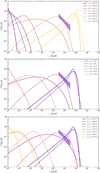 |
Fig. 1. Proton energy spectra ϵ2 dncor/dϵ (per log-interval of energy) vs. proton energy ϵ predicted by stochastic acceleration in a turbulent corona, starting from mono-energetic protons with a Lorentz factor of γ0 ∼ 1. In each panel, the solid line corresponds to a solution obtained by integrating the Fokker-Planck equation up to time τadv = rco/vadv (model (1) including energy losses, advection, and escape as described in the text), and the dashed line shows the corresponding solution for the same parameters for the generalized Fermi model described by Eq. (5) (model (2)). In all panels, rco is set to 30rg, and in the top and middle panels, vadv ≃ 0.02 c. The upper panel shows the dependence on vA, assuming otherwise a coherence length scale for the turbulence ℓc = 10 rg and an advection velocity vadv = 0.02 c. From left to right, as indicated, vA/c = 0.05, vA/c = 0.10, vA/c = 0.20, and vA/c = 0.40. The middle panel examines the dependence on ℓc, assuming otherwise vA/c = 0.20 and vadv/c = 0.02. From right to left, as indicated, ℓc = 3 rg, ℓc = 10 rg, and ℓc = 30 rg. The bottom panel examines the influence of advection, characterized here by the advection velocity vadv (which sets the advection timescale τadv ≡ rco/vadv), assuming otherwise vA/c = 0.20 and ℓc = 3 rg. From right to left, as indicated, vadv/c = 0.02, vadv/c = 0.05, vadv/c = 0.16 and a (more extreme) case vadv/c = 0.49. The butterfly indicates the range of values needed to reproduce a neutrino spectrum as observed by IceCube for NGC 1068. The energy density spectrum is expressed in units of the background plasma pressure (see Sect. 2.1). In these units, each individual spectrum has been normalized to an integrated fraction of unity for the sake of illustration. |
The trivial observation that hardly any of the spectra fit this butterfly diagram can be misleading. The important point is that the predicted spectra are extremely sensitive to the choice of parameters. This is easily understood, noting that for Dϵϵ ∝ ϵ2, the mean energy increases exponentially fast in time, that is, ⟨ϵ⟩∝exp(4νacct), with νacc ≡ Dϵϵ/ϵ2 the acceleration rate defined earlier. Consequently, in a fixed time interval t = τadv over which νacct ≫ 1 (needed to achieve acceleration to high energies), changing νacc by a factor of a few changes the maximum energy by orders of magnitude. The dependence of νacc on the parameters is recalled above, νacc ∝ vA2/ℓc. We assumed δB/B ≳ 1, otherwise νacc should be further suppressed by a factor (δB/B)2. The dependence on the advection velocity is also easily understood because the number of e-folds of the increase in the maximum energy scales as νaccτadv ∝ 1/vadv. From this, we can also infer the dependence on the scale of the corona. The spectra that reach PeV energies are cut off because of catastrophic hadronic losses. Other spectra are cut off because of the limited time they spend in the corona.
Clearly, parameter values that fit the inferred butterfly diagram might be found, and examples are shown below. This comes at the price of some fine-tuning, however. One important corollary is that under the above assumptions, we do not expect all AGNs, even those with a similar X-ray luminosity, to produce neutrinos with a similar spectrum. If the physical conditions that dictate the rate of acceleration (e.g., vA) show an extended distribution over the neutrino-emitting AGN subpopulation, the population as a whole is instead expected to produce an extended neutrino energy spectrum, from ≲GeV to ∼0.1 PeV. This has consequences for our prediction of the diffuse flux from this population of AGNs and for the modeling of the spectrum of a given source, as we discuss further in Sect. 3.
Another important lesson drawn from Fig. 1 is that fitting the inferred proton spectrum raises an energy budget issue, as noted earlier (Sect. 2.1), which also represents an intriguing coincidence. Namely, in order to match the flux, we must inject a tiny fraction of the thermal plasma into stochastic acceleration, such that after energization by a factor ∼105, its pressure is comparable to that of its parent population. If more particles had been injected, the energy requirement would have become excessive, while in the opposite case, the proton flux falls short of the required flux. Moreover, if suprathermal particles carry an energy density comparable to that in the thermal component, they must backreact on the flow, and in particular, damp the turbulence that feeds them in energy. In this situation, stochastic acceleration becomes nonlinear and self-regulated by damping (Eilek 1979; Eichler 1979b; Litvinenko 2012; Kakuwa 2016; Lemoine et al. 2024). We discuss this possibility further in Sect. 3.
Alternatively, the turbulent corona might not shape the entire proton spectrum, but only part of it, and protons escaping the corona might be further accelerated in the sheared velocity flows at the base of the jet. We first discuss how this shear acceleration can be implemented, and we then examine the general combination of the two scenarios in Sect. 3.
2.3. Particle acceleration in sheared flows
Accreting black hole systems are known to drive relativistic jets and winds, and thereby provide an environment that is conducive to shear-type particle acceleration (e.g., Kimura et al. 2018; Rieger 2019; Lemoine 2019; Rieger & Duffy 2022; Webb et al. 2023; Wang et al. 2024). This might provide a complementary mechanism for proton energization if turbulent acceleration in the corona were to saturate at multi-TeV energies. To be efficient, shear acceleration commonly requires seed injection of energetic particles, which is in line with a hierarchical acceleration scenario. In our context, we envisaged that the black hole vicinity supports a fast, sheared outflow; for example, that the hot X-ray emitting corona forms the base of an outward-moving jet, which may be supported by radiation pressure or be driven magnetically (e.g., Beloborodov 1999; Malzac et al. 2001; Merloni & Fabian 2002; King et al. 2017; Liska et al. 2022; Poutanen et al. 2023; Dexter & Begelman 2024; Sridhar et al. 2025). For the prototype Seyfert galaxy NGC 1068, jet-like features are indeed apparent on larger scales, although jet speeds are most likely nonrelativistic (≲0.1 c) on scales of several dozen parsec (∼107 rg) from the nucleus (Gallimore et al. 1996; Roy et al. 2000; May & Steiner 2017). Part of its observed gamma-ray emission may in fact be related to the jet (e.g., Lenain et al. 2010; Salvatore et al. 2024). The radio-inferred (large-scale and time-averaged) jet power is about Ljet ∼ 1043 erg/s (Padovani et al. 2024). On the other hand, the minimum (isotropic-equivalent) cosmic-ray power required to account for the observed neutrino emission is about several 1042 erg/s (e.g., Murase 2022, see also Appendix A). If part of this emission is indeed related to the outflow, even if it were relativistically boosted, it seems conceivable that cosmic-ray acceleration may contribute to the deceleration of the flow (viscous drag) as it propagates outward. We did not include this possible backreaction and self-regulation of the acceleration process in our modeling, but we note that it may impact on the bulk flow profile (e.g., shear broadening) and on the turbulence generation.
For reference, we explore a model below in which turbulent acceleration in the corona saturates at γp ≤ 104 (10 TeV) either due to vA ≲ 0.1 c or ℓc ≫ rg in the corona. The corona thus sustains a reservoir of energetic seed particles that can diffuse into the outflow and experience further jet-shear acceleration. In this process, acceleration is related to a particle that effectively samples the velocity difference while it is scattered across a shearing flow (Rieger 2019). For simplicity, we considered a collimated mildly relativistic outflow or jet, with a Lorentz factor of γj ≡ 1/(1 − uz2/c2)1/2 ≲ 3, characterized by a lateral velocity shear uz(r) with a width of  . Energetic protons undergoing shear acceleration are subjected to radiative losses and diffusive escape (see Appendix A). For the phenomenological application, the acceleration process can be modeled through a diffusive Fokker-Planck equation for n(ϵ) of the type Eq. (1), with mean momentum diffusion coefficient
  , where for energetic protons, ϵ = pc = γmpc2. The coefficient
  can be obtained from the local (r-dependent) shear coefficient Dp(r) = (1/15)γj(r)4(∂uz/∂r)2λ/c by suitable spatial averaging, for example, ag = (2/3)(c/Δr)2/w with w = 116 (ln[(1 + β0)/(1 − β0)])−2 in the case of a linearly decreasing shear flow profile with a maximum (spine) speed β0 = (1 − 1/γj, max2)1/2 (Rieger & Duffy 2019, 2022). In the former expression, λ = cτc = η (Δr)(rL/Δr)1/3 denotes the scattering mean free path (rL the gyroradius), for which we took a scaling with η = 2, following Rieger & Duffy (2019) and Wang et al. (2023) (see also Appendix A). Particles can escape from the acceleration region either due to cross-field diffusion (laterally), that is, τesc = (Δr)2/(2κ) with κ = λc/3, or through advective transport (along z), τadv, z. The accelerated particle distribution on scales of the corona is of interest here. While shear acceleration likely continues to operate along the jet, we considered the former to dominate hadronic interactions and thus neutrino production. Accordingly, we approximated advective escape by
  , with ⟨uz⟩ the mean velocity (corresponding to β0c/2), and
  lower than a few here to ensure that the target photon density is high enough. As before (Sect. 2.2), this was implemented as a constraint on the time available for particle acceleration. Figure 2 presents exemplary proton energy spectra as a function of time (in units of τc(γ0)) assuming that seed protons are continuously injected with a Lorentz factor of γ0 = 104 into a shearing flow with γj = 3, B = 50 G,
  and
and  , assuming a corona size of rco = 30 rg.
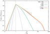 |
Fig. 2. Exemplary time-dependent proton energy distribution obtained from jet-shear acceleration with a Fokker-Planck model assuming continuous injection of seed protons with γ0 = 104. As a result of advective escape, the predicted particle spectrum will appear somewhat softer (red, t = τadv, z) compared to the otherwise quasi steady-state distribution (yellow). The gray shaded region illustrates the spectral characteristics required to reproduce the neutrino emission for NGC 1068 as measured by IceCube. |
In general, the predicted spectra are sensitive to the choice of parameters, for example, the time available for particle acceleration (set by τadv, z). One important corollary of the latter is that shear modeling imposes constraints on the size and geometry of the corona. In addition, the required maximum outflow speed to model the CR parent distribution behind the IceCube neutrino spectrum is sensitive to the flow profile. In comparison to power-law or Gaussian-type velocity profiles, a linearly decreasing shear flow profile requires higher speeds to reproduce hard particle spectra. For the former, γj ≤ 2 are sufficient (Rieger & Duffy 2022). This suggests that mildly relativistic outflow speeds are sufficient to account for an inferred proton spectrum such as in NGC 1068. Jet deceleration due to cosmic-ray-induced viscous drag, interaction with a central magnetic or cosmic-ray-driven wind, along with the efficient generation of turbulence and entrainment of ambient material, may explain the relatively low velocity of the jet in NGC 1068 on larger scales. Our current model at this stage remains exploratory in nature since the innermost outflow characteristics in Seyfert-2 AGNs remain uncertain, and since we neglected a possible shear contribution due to flow rotation. The latter may facilitate transport of angular momentum from the underlying accretion flow, and it night in effect contribute to further spectral hardening (Rieger & Mannheim 2002). In general, while particle acceleration in sheared flows will not lead to a canonical power-law shape, faster flows will (ceteris paribus) result in harder particle spectra. This agrees with the above corollary, according to which not all X-ray bright Seyfert AGNs are expected to have similar neutrino spectra.
3. Discussion
In the preceding section, we have examined the general features of particle acceleration in a turbulent corona, with possible reacceleration in the sheared velocity flow outside of this corona. We interpret these results here and combine them to suggest ways in which the generic proton spectrum inferred from IceCube observations can be reproduced, and we draw conclusions regarding the phenomenology. More specifically, we investigated the following three scenarios.
First, we considered pure stochastic acceleration in the turbulent corona, as modeled in Sect. 2.2, and we demonstrate that a reasonable set of parameters can be found to reproduce the high-energy general slope. This was known from previous studies (e.g., Murase et al. 2020b; Inoue et al. 2020; Kheirandish et al. 2021; Murase 2022; Eichmann et al. 2022; Fiorillo et al. 2024b); the main novelty here lies in the transport equation we used, in particular, for the implementation of generalized Fermi acceleration, and in the treatment of escape and advection. As noted above (Sect. 2.2), matching the spectrum requires some tuning in terms of the physical parameters and in terms of flux normalization. This suggests that other sources might display vastly different neutrino spectra even for otherwise similar coronal X-ray luminosities. Interestingly, the IceCube experiment reports differing spectra from other Seyfert galaxies (e.g., Abbasi et al. 2025, 2024). In the case of NGC 4151 (d ∼ 16 Mpc), for instance, the characteristic neutrino energy seems higher by a factor ∼5, and the high-energy slope is slightly harder than in NGC 1068.
The spectra obtained in this first scenario are shown in the top panel of Fig. 3. While the parameters are the same for the two spectra shown, namely rco = 30 rg, ℓc = 10 rg, vadv = 0.02 c and vA ≃ 0.2 c, their flux normalizations are different. The ratio of integrated energy density of suprathermal particles to background plasma pressure is ≃4.3 for model (1) and 1.0 for model (2). Because the ratio of the pressures is lower by a factor 3, the dynamical influence of the suprathermal particles should not be ignored in model (1). This further motivates the need to study the impact of backreaction on the turbulence, which is discussed further below. Finally, we note that other sets of parameters might be found, for example, a lower Alfvén velocity with a smaller coherence length scale. However, the general spectral shape should be preserved.
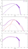 |
Fig. 3. Proton energy spectra dup/dlnϵ ≡ ϵ2 dn/dϵ vs. proton energy ϵ for three characteristic scenarios described in the text. For each panel, the energy density distribution is shown in units of the background plasma pressure. Top panel: Stochastic acceleration in the turbulent corona, with a characteristic Alfvénic velocity vA ≃ 0.2 c (see text for details), for model (1) and (2), corresponding to the solid and dashed lines, respectively. Middle panel: Combination of stochastic acceleration in the corona with shear acceleration at the base of the jet (see text for the details of the physical parameters). The stochastic contribution is indicated by dotted lines, the shear contribution by dashed lines, and the sum of the two by solid lines. The different colors correspond to models (1) and (2). For the top and middle panels, the normalization of the energy density in accelerated particles has been fixed in order to reproduce the inferred proton flux. Bottom panel: Modeling of stochastic acceleration, accounting for self-regulation by particle feedback on the turbulence (damping), for a characteristic Alfvén velocity vA ≃ 0.2 c. The plasma β parameter is 0.5 (see Appendix A). |
In a second scenario, we investigated the interplay of turbulent and shear acceleration. Shear acceleration requires high-energy seed particles because the rate at which acceleration proceeds increases with the particle mean free path (e.g. Rieger 2019; Rieger & Duffy 2022; Webb et al. 2023; Wang et al. 2024), so that in the absence of turbulent preacceleration, this mechanism would be effectively inefficient. In our setting, particles that have been preaccelerated in a turbulent corona are assumed to enter a region of sheared velocity flow, either through diffusive escape or through advection from the corona. For clarity, we concentrated on the latter case, in which particles first cross a turbulent corona and then enter a region of sheared velocity flow. There is a sizable uncertainty here, not only on the overall geometry of the problem, but also on the exact fraction of particles that are able to transit from one region to the next, as well as on the parameters characterizing the shear flow. We thus used the same parameters as in Sect. 2.3 to describe the base of a mildly relativistic jet. To model the particle spectra, we convolved the Green function, which characterizes shear acceleration Gshear(ϵ; ϵ′, τshear), that is, the probability of jumping from ϵ′ to ϵ over the timescale τshear spent in the shear region, with an injection distribution that describes the time-dependent particle spectrum of the turbulent region. Denoting the latter as dnturb/dϵ, we write the stationary spectrum in the shear region as

with τadv, z the advection time in the sheared region, as before, and
where dninj/dϵ″ characterizes (Sect. 2.2) the injection spectrum at the entry of the turbulent region, as before. We introduced a ratio vadv/vshear as a prefactor in Eq. (6) to account for the difference in advection velocity of each region (conservation of particle current). We assumed that the shear region extends over rco and took ⟨uz⟩=β0 c/2 ≃ 0.5 c.
Finally, the total stationary spectrum was obtained as the sum of the spectra in each region, dncor/dϵ (Eq. (3)) and dnshear/dϵ (Eq. (6)). Although the overall normalization was left here as a free parameter, the relative normalization of these two was fixed by the volume of each region. The result is shown in the middle panel of Fig. 3. This figure illustrates that the shear contribution acts as re-energization of the seed population produced by turbulent acceleration. This shapes an effective power-law tail close to ∝ϵ−3 (per number), which is close to the tail inferred from IceCube observations. The parameters we adopted are the same as in Sect. 2.3 for the shear layer, and vA = 0.20 c, vadv = 0.02 c, ℓc = 10 rg, and rco = 30 rg as in Fig. 1 for the stochastic acceleration. For simplicity, we ignored possible boosting effects for the shear contribution. In general, if the shear flow were subrelativistic, shear acceleration would become too slow to have any effect, as quantified by the dependence of the diffusion coefficient on the Lorentz factor of the flow (Sect. 2.3). We also note that we considered a scenario in which particles were injected at one boundary of the corona, accelerated by turbulence, and then advected into the shear layer. If we had considered that a fraction of particles could be advected into the black hole instead of the jet, the shear contribution would have been reduced. Similarly, if we had assumed that particles were injected into stochastic acceleration uniformly throughout the corona (see Sect. 2.2), then the spectrum injected into the shear process would have been the steady-state spectrum dncor/dϵ instead of the spectrum discussed above. The overall shear contribution would have been effectively reduced in this case as well, and, a normalization of the overall spectrum to the inferred values without invoking boosting would have implied stronger energy requirements. In our case, the ratios of the integrated energy density in suprathermal particles to background plasma pressure are 4.1 and 2.7 for models (1) and (2), respectively.
Finally, we investigated the consequences of self-regulation of the acceleration process by turbulent damping. Because in the two scenarios discussed previously, the pressure carried by the accelerated particles is comparable to that in the background plasma, this last scenario appears to be quite likely. We also note that in the above cases, the flux normalization was set in such a way as to reproduce the normalization inferred from IceCube observations, and as mentioned previously, this amounts to selecting a precise fraction of particles that are extracted from the thermal pool are and then accelerated to high energies. We thus accounted for the backreaction of the accelerated particles on the turbulence following the prescriptions of Lemoine et al. (2024). As detailed therein, backreaction becomes effective when the rate at which particles draw energy from the turbulent cascade exceeds the energy at which the cascade is replenished by energy injection. The former rate can be written ∼νaccup (up is the suprathermal proton energy density), with νacc ∼ vA2/(cℓc), while the latter reads ∼(vA/ℓc) uB (uB is the magnetic energy density). Turbulent damping therefore becomes effective when up/uB ∼ c/vA. When we assume a plasma βp unity (see Appendix A), this also means that damping takes place when  here. When the particles start to damp the turbulence, the stochastic acceleration rate stalls, and acceleration becomes self-regulated.
To fix the parameters, we assumed that the cascade rate on the outer scale was 0.5 vA/ℓc, as expected on general grounds. We used rco = 30 rg, vadv = 0.02 c, and ℓc = 10 rg as before, and we injected particles at γ0 ∼ 1 as before, with an energy density lower by a factor of four than contained in the magnetized turbulence. We then tracked their acceleration using the two effective models (a) and (b) described by Lemoine et al. (2024), which mimic models (1) and (2) above. In detail, model (a) corresponds to the Fokker-Planck model and assumed vA = 0.21 c, while model (b) describes advection in momentum space of a broken power-law spectrum assuming vA = 0.28 c. Finally, we computed the global stationary spectrum over the corona by integrating the time-dependent spectra as in Eq. (3). The resulting spectrum is shown in the lower panel of Fig. 3. We stress that in this scenario, no ad hoc normalization of the energy content was adopted. This energy content is dictated by the backreaction of particles on the turbulence, which, as discussed above, implies that the total energy density in suprathermal particles must be about pgasc/vA. In units of pgas, the energy density associated with the particle spectra shown in Fig. 3 is 3.4 in model (a) and 4.1 in model (b). The general shape of the spectrum does not depend much on the method used to carry out the integration. The key parameter that determines whether the overall flux can match the detailed spectrum at energies 30 − 300 TeV is the Alfvén velocity (more generally, νaccτadv), which determines the location of the high-energy cutoff. The fact that the inferred spectrum can be reproduced at the price of reasonable parameters without an arbitrary normalization provides additional support and motivation for this scenario.
The global spectral shape of self-regulated acceleration can be understood as follows. In a first stage, particles are accelerated as in the test-particle picture of the first scenario that we investigated previously in this section. This occurs as long as the energy carried by the suprathermal particles remains below the threshold for backreaction, and it explains the similarity of the spectral slopes at low energies with that shown in the upper panel of Fig. 3. When feedback becomes efficient, acceleration stalls at the momentum determining the peak of the energy distribution, while particles with a higher momentum can continue to be accelerated because they interact with wavelength modes of larger scales that have not yet been damped. This tends to shape time-dependent energy spectra that are approximately flat at high energies. The average of these time-dependent spectra over the crossing time of the corona, accounting for energy and escape losses, then shapes the observed spectrum, similar to or slightly steeper than −2 in slope (per number). One phenomenological implication of this modeling is that in order to match a spectrum steeper than −2 in slope, the spectrum should be close to the cutoff region, that is, it should reveal increasing curvature toward higher energies. For higher acceleration rates or higher νaccτadv, the maximum energy is pushed to higher values, and the spectrum in a given region therefore approaches −2 in slope.
We therefore recall the dependence of the cutoff location on νaccτadv. However, if this combination of parameters were inhomogeneous throughout the corona, for example, because the Alfvénic velocity itself varied in space (as proposed in the context of X-ray binaries; see Nättilä 2024), the sharp high-energy cutoff would be replaced by a softer dependence associated with the tail of values of νaccτadv. A more general interpretation of the proton spectrum is therefore called for, in which the flux level is determined by backreaction as modeled above, while the slope of the spectrum in the region probed by IceCube is dictated by the distribution of the acceleration rates (and advection times) experienced by the particle population. We defer the detailed investigation of this scenario to future work.
4. Conclusions
We have investigated scenarios of stochastic particle acceleration in a turbulent magnetized black hole corona and in the sheared velocity flow at the base of the jet to examine to which degree they can account for the proton energies inferred from IceCube neutrino observations of the Seyfert prototype NGC 1068, namely ϵ ∼ 30 − 300 TeV, and for the overall level of the energy density. To this end, we used recent results for stochastic particle acceleration in turbulence and paid particular attention to the transport equation, that is, we considered the influence of turbulent transport on escape losses and incorporated advection losses as a time limit on particle acceleration (Sect. 2.2). In Sect. 3 we compared three characteristic scenarios to the proton spectrum inferred in the case of NGC 1068 to conclude the following.
In a first scenario, which portrayed particle acceleration in the test-particle limit in a turbulent corona, we confirmed previous results that suggested that a characteristic Alfvénic velocity vA ≃ 0.1 − 0.2 c for a coherence length ℓc ∼ 3 − 10 rg can reproduce the general shape of the observed spectrum. However, this comes at the cost of an ad hoc normalization of the proton spectrum up to an appreciable fraction of the background plasma pressure, which in some cases exceeds unity. In terms of phenomenology, the spectrum is expected to reveal an increasingly strong curvature toward higher energies.
In a second scenario, we investigated the possibility that stochastic acceleration consumes less energy, but is completed by a phase of reacceleration in the sheared velocity flow at the base of a mildly relativistic jet. This flow, whether interpreted as an inner disk wind or jet wall, was envisioned to be launched from small radii well inside the corona; beyond this, however, it does not favor any specific model for the corona geometry. While this scenario admittedly introduces new parameters into the problem, it shows that shear reacceleration can play a role and lead to a satisfactory fit to the observed spectrum for a reasonable choice of parameters. In particular, depending on the conditions for escape, the particle distribution might extend to even higher energies, as shown in Fig. 3. In our context, the relative importance of shear acceleration depends on the magnitude of the shear, which determines the rate at which particles are re-energized in the jet boundary layer, just as it depends on the advection velocity in the corona. Similarly to the first scenario, the overall flux normalization was chosen freely and required that the energy density in high-energy protons lies close to the overall pressure of the background plasma.
This apparent coincidence is intriguing with respect to particle injection into the stochastic process, because it means that a specific fraction of particles must be extracted from the thermal pool that is smaller by some orders of magnitude than unity, yet such that after acceleration, it carries an amount of energy that is comparable to the pressure of their parent population. Based on the observation that the gas pressure is βp times the magnetic energy density uB, and that βp ∼ 1, this observation may indicate that the acceleration process is as efficient as can be, that is, that the high-energy particles extract as much energy as they can from the turbulent cascade.
We therefore examined a third scenario in which turbulent acceleration was self-regulated by this feedback, which takes the form of damping of the turbulent cascade in the inertial range. In this scenario, the problem was fixed by the rate at which turbulent energy is injected on the outer scale ℓc, with a generic value of ∼uBvA/ℓc. Adopting this rate and characteristic Alfvénic velocities as above, solving for the concomitant dynamical evolution of the turbulence and of the accelerated particles, we were able to reproduce the inferred proton spectra without having to specify the flux normalization. We did not explore the possibility that the accelerated particles might provide a backreaction at a more global (hydrodynamical) level on the structure of the flow itself, such as the liftoff of the hydrostatic equilibrium in the corona or jet deceleration in the case of shear acceleration. These issues clearly deserve further investigation.
This self-regulated acceleration process becomes operative provided the fraction χ0 of particles that are extracted from the thermal pool and injected into stochastic acceleration verifies  in terms of the plasma β parameter (βp), the Alfvénic velocity vA (here playing the role of the characteristic eddy velocity on the outer scale of the turbulence), ϵmax the maximum energy of the nonthermal energy spectrum, and
  the mean thermal energy. If the injection fraction χ0 is smaller than the above, feedback has not set in by the time the particles are accelerated to ϵmax, and hence, particle acceleration proceeds as in a test-particle picture. However, if
  , that is, if particles are able to reach high energies, feedback becomes natural, and the high-energy part of the accelerated spectrum then depends weakly on the details of the injection.
In this scenario of self-regulated stochastic acceleration, the source outputs as much energy as available in high-energy protons and achieves approximate equipartition between the supra-thermal proton and turbulent magnetic energy densities. This feature is all the more appealing in the context of high apparent neutrino luminosities such as were reported for NGC 1068. One direct consequence of this is that the overall neutrino luminosity of the source is not only controlled by the X-ray luminosity, which governs p − γ interactions, but also by the magnetic energy content. Our study indicates that other parameters are likely to influence the neutrino spectrum. We notably remarked that the maximum energy is strongly sensitive to the acceleration rate, for example, to the Alfvén velocity, the coherence length, and to the advection timescale through the corona. This dependence arises because the mean particle energy increases exponentially fast in turbulent acceleration up to a number of e-folds that is set by a combination of these parameters. An important corollary of this is that different sources might exhibit different spectra. An alternative way of viewing this strong dependence is that if the corona were inhomogeneous in terms of vA (e.g.), the final spectrum is a sum of spectra obtained for differing vA, or in other words, the final spectrum is shaped by the distribution of vA (and other parameters) in the corona. Overall, it is therefore tempting to interpret the flux level as the consequence of self-regulated particle acceleration by turbulence damping (or possibly, viscous damping of the sheared velocity flow), and the general slope of the spectrum as given by the distribution of acceleration rates within the corona.
Finally, as pointed out to us by A. Beloborodov and A. Levinson, the possibility of turbulence damping introduces new issues. In particular, it may jeopardize the energization of electrons, which is expected to power the X-ray luminosity of the corona. We note, however, that in our description, the advection of particles through the corona effectively leads to stratification in terms of mean energy because time-dependent spectra also depend on the position. Close to the boundary where particles are injected into the corona, turbulence is therefore not affected, and electron energization is efficient. Furthermore, the damping of turbulence on scales of ≲l, for instance, does not prevent the formation of reconnection layers on scales ∼l, which offer ancillary energization channels. In an electron-ion plasma, reconnection can energize particles to a mean energy ∼(1 + σ)mpc2, where the magnetization parameter σ ≃ (vA/c)2 (at σ ≲ 1) denotes the ratio of the magnetic to plasma energy density (Werner et al. 2018). While turbulent reconnection is therefore not expected to affect the proton spectrum at the highest energies for moderate values of σ, it may contribute to electron energization. In a conservative model, it suffices to energize electrons to Lorentz factors γe < 102 to power the X-ray luminosity, and these electrons behave as mildly or subrelativistic protons. Overall, it appears reasonable to assume that the electrons can indeed be energized as needed in spite of turbulent damping. A detailed investigation of this question will form the basis of future work.
Acknowledgments
It is a pleasure to thank A. Beloborodov and A. Levinson, F. Oikonomou and E. Peretti as well as the members of the CN-6 connector of the Munich Excellence Cluster ORIGINS (in particular, P. Padovani, X. Rodrigues, and E. Resconi) for stimulating discussions. FMR acknowledges support by a DFG grant (RI 1187/8-1) and the kind hospitality of the IAP Paris.
References
- Abbasi, R., Ackermann, M., Adams, J., et al. 2024, ArXiv e-prints [arXiv:2406.07601] [Google Scholar]
- Abbasi, R., Ackermann, M., Adams, J., et al. 2025, ApJ, 981, 131 [Google Scholar]
- Aharonian, F., & Neronov, A. 2005, ApJ, 619, 306 [CrossRef] [Google Scholar]
- Aharonian, F. A., Belyanin, A. A., Derishev, E. V., Kocharovsky, V. V., & Kocharovsky, V. V. 2002, Phys. Rev. D, 66, 023005 [Google Scholar]
- Ambrosone, A. 2024, JCAP, 2024, 075 [Google Scholar]
- Beloborodov, A. M. 1999, MNRAS, 305, 181 [Google Scholar]
- Berezinskii, V. S., Bulanov, S. V., Dogiel, V. A., & Ptuskin, V. S. 1990, Astrophysics of Cosmic Rays (Amsterdam: North-Holland) [Google Scholar]
- Berezinsky, V. S., & Ginzburg, V. L. 1981, Int. Cosmic Ray Conf., 1, 238 [Google Scholar]
- Bresci, V., Lemoine, M., Gremillet, L., et al. 2022, Phys. Rev. D, 106, 023028 [Google Scholar]
- Brunetti, G., & Lazarian, A. 2016, MNRAS, 458, 2584 [Google Scholar]
- Comisso, L., & Sironi, L. 2018, Phys. Rev. Lett., 121, 255101 [NASA ADS] [CrossRef] [Google Scholar]
- Comisso, L., & Sironi, L. 2019, ApJ, 886, 122 [Google Scholar]
- Comisso, L., & Sironi, L. 2022, ApJ, 936, L27 [NASA ADS] [CrossRef] [Google Scholar]
- Das, A., Zhang, B. T., & Murase, K. 2024, ApJ, 972, 44 [NASA ADS] [CrossRef] [Google Scholar]
- De Villiers, J.-P., Hawley, J. F., & Krolik, J. H. 2003, ApJ, 599, 1238 [NASA ADS] [CrossRef] [Google Scholar]
- De Villiers, J.-P., Hawley, J. F., Krolik, J. H., & Hirose, S. 2005, ApJ, 620, 878 [NASA ADS] [CrossRef] [Google Scholar]
- Demidem, C., Lemoine, M., & Casse, F. 2020, Phys. Rev. D, 102, 023003 [Google Scholar]
- Dermer, C. D., Miller, J. A., & Li, H. 1996, ApJ, 456, 106 [Google Scholar]
- Dexter, J., & Begelman, M. C. 2024, MNRAS, 528, L157 [Google Scholar]
- Di Matteo, T., Blackman, E. G., & Fabian, A. C. 1997, MNRAS, 291, L23 [Google Scholar]
- Eichler, D. 1979a, ApJ, 232, 106 [Google Scholar]
- Eichler, D. 1979b, ApJ, 229, 413 [Google Scholar]
- Eichmann, B., Oikonomou, F., Salvatore, S., Dettmar, R.-J., & Tjus, J. B. 2022, ApJ, 939, 43 [NASA ADS] [CrossRef] [Google Scholar]
- Eilek, J. A. 1979, ApJ, 230, 373 [CrossRef] [Google Scholar]
- Fabian, A. C., Lohfink, A., Kara, E., et al. 2015, MNRAS, 451, 4375 [Google Scholar]
- Fang, K., Lopez Rodriguez, E., Halzen, F., & Gallagher, J. S. 2023, ApJ, 956, 8 [NASA ADS] [CrossRef] [Google Scholar]
- Farrar, G. R., & Piran, T. 2014, ArXiv e-prints [arXiv:1411.0704] [Google Scholar]
- Fiorillo, D. F. G., Petropoulou, M., Comisso, L., Peretti, E., & Sironi, L. 2024a, ApJ, 961, L14 [NASA ADS] [CrossRef] [Google Scholar]
- Fiorillo, D. F. G., Comisso, L., Peretti, E., Petropoulou, M., & Sironi, L. 2024b, ApJ, 974, 75 [NASA ADS] [CrossRef] [Google Scholar]
- Gallimore, J. F., Baum, S. A., O’Dea, C. P., & Pedlar, A. 1996, ApJ, 458, 136 [Google Scholar]
- Guépin, C., Kotera, K., Barausse, E., Fang, K., & Murase, K. 2018, A&A, 616, A179 [NASA ADS] [CrossRef] [EDP Sciences] [Google Scholar]
- Halzen, F. 2023, ArXiv e-prints [arXiv:2305.07086] [Google Scholar]
- IceCube Collaboration (Abbasi, R., et al.) 2022, Science, 378, 538 [CrossRef] [PubMed] [Google Scholar]
- Inoue, Y., & Doi, A. 2018, ApJ, 869, 114 [Google Scholar]
- Inoue, Y., Khangulyan, D., & Doi, A. 2020, ApJ, 891, L33 [Google Scholar]
- Inoue, Y., Takasao, S., & Khangulyan, D. 2024, PASJ, 76, 996 [Google Scholar]
- Isliker, H., Vlahos, L., & Constantinescu, D. 2017, Phys. Rev. Lett., 119, 045101 [NASA ADS] [CrossRef] [Google Scholar]
- Kakuwa, J. 2016, ApJ, 816, 24 [NASA ADS] [CrossRef] [Google Scholar]
- Kammoun, E., Lohfink, A. M., Masterson, M., et al. 2024, Front. Astron. Space Sci., 10, 1308056 [NASA ADS] [CrossRef] [Google Scholar]
- Kamraj, N., Harrison, F. A., Baloković, M., Lohfink, A., & Brightman, M. 2018, ApJ, 866, 124 [CrossRef] [Google Scholar]
- Kamraj, N., Brightman, M., Harrison, F. A., et al. 2022, ApJ, 927, 42 [NASA ADS] [CrossRef] [Google Scholar]
- Kara, E., García, J. A., Lohfink, A., et al. 2017, MNRAS, 468, 3489 [NASA ADS] [CrossRef] [Google Scholar]
- Kardashev, N. S. 1962, Soviet Astron., 6, 317 [NASA ADS] [Google Scholar]
- Kempski, P., Fielding, D. B., Quataert, E., et al. 2023, MNRAS, 525, 4985 [NASA ADS] [CrossRef] [Google Scholar]
- Kheirandish, A., Murase, K., & Kimura, S. S. 2021, ApJ, 922, 45 [NASA ADS] [CrossRef] [Google Scholar]
- Kimura, S. S., Murase, K., & Zhang, B. T. 2018, Phys. Rev. D, 97, 023026 [CrossRef] [Google Scholar]
- Kimura, S. S., Tomida, K., & Murase, K. 2019a, MNRAS, 485, 163 [Google Scholar]
- Kimura, S. S., Murase, K., & Mészáros, P. 2019b, Phys. Rev. D, 100, 083014 [Google Scholar]
- King, A. L., Lohfink, A., & Kara, E. 2017, ApJ, 835, 226 [NASA ADS] [CrossRef] [Google Scholar]
- Lemoine, M. 2019, Phys. Rev. D, 99, 083006 [Google Scholar]
- Lemoine, M. 2021, Phys. Rev. D, 104, 063020 [NASA ADS] [CrossRef] [Google Scholar]
- Lemoine, M. 2022, Phys. Rev. Lett., 129, 215101 [NASA ADS] [CrossRef] [Google Scholar]
- Lemoine, M. 2023, J. Plasma Phys., 89, 175890501 [CrossRef] [Google Scholar]
- Lemoine, M., & Malkov, M. A. 2020, MNRAS, 499, 4972 [NASA ADS] [CrossRef] [Google Scholar]
- Lemoine, M., Murase, K., & Rieger, F. 2024, Phys. Rev. D, 109, 063006 [Google Scholar]
- Lenain, J. P., Ricci, C., Türler, M., Dorner, D., & Walter, R. 2010, A&A, 524, A72 [NASA ADS] [CrossRef] [EDP Sciences] [Google Scholar]
- Levinson, A., & Boldt, E. 2002, Astropart. Phys., 16, 265 [Google Scholar]
- Liska, M. T. P., Musoke, G., Tchekhovskoy, A., Porth, O., & Beloborodov, A. M. 2022, ApJ, 935, L1 [NASA ADS] [CrossRef] [Google Scholar]
- Litvinenko, Y. E. 2012, A&A, 544, A94 [NASA ADS] [CrossRef] [EDP Sciences] [Google Scholar]
- Liu, B. F., Mineshige, S., & Shibata, K. 2002, ApJ, 572, L173 [CrossRef] [Google Scholar]
- Lynn, J. W., Quataert, E., Chandran, B. D. G., & Parrish, I. J. 2014, ApJ, 791, 71 [Google Scholar]
- Malzac, J., Beloborodov, A. M., & Poutanen, J. 2001, MNRAS, 326, 417 [NASA ADS] [CrossRef] [Google Scholar]
- May, D., & Steiner, J. E. 2017, MNRAS, 469, 994 [NASA ADS] [CrossRef] [Google Scholar]
- Mbarek, R., Philippov, A., Chernoglazov, A., Levinson, A., & Mushotzky, R. 2024, Phys. Rev. D, 109, L101306 [CrossRef] [Google Scholar]
- Merloni, A., & Fabian, A. C. 2001, MNRAS, 321, 549 [NASA ADS] [CrossRef] [Google Scholar]
- Merloni, A., & Fabian, A. C. 2002, MNRAS, 332, 165 [NASA ADS] [CrossRef] [Google Scholar]
- Murase, K. 2022, ApJ, 941, L17 [NASA ADS] [CrossRef] [Google Scholar]
- Murase, K., Kimura, S. S., Zhang, B. T., Oikonomou, F., & Petropoulou, M. 2020a, ApJ, 902, 108 [NASA ADS] [CrossRef] [Google Scholar]
- Murase, K., Kimura, S. S., & Mészáros, P. 2020b, Phys. Rev. Lett., 125, 011101 [Google Scholar]
- Murase, K., Karwin, C. M., Kimura, S. S., Ajello, M., & Buson, S. 2024, ApJ, 961, L34 [NASA ADS] [CrossRef] [Google Scholar]
- Nättilä, J. 2024, Nat. Commun., 15, 7026 [Google Scholar]
- Neronov, A., Savchenko, D., & Semikoz, D. V. 2024, Phys. Rev. Lett., 132, 101002 [NASA ADS] [CrossRef] [Google Scholar]
- Padovani, P., Resconi, E., Ajello, M., et al. 2024, Nat. Astron., 8, 1077 [Google Scholar]
- Pecora, F., Servidio, S., Greco, A., et al. 2018, J. Plasma Phys., 84, 725840601 [Google Scholar]
- Pezzi, O., Blasi, P., & Matthaeus, W. H. 2022, ApJ, 928, 25 [NASA ADS] [CrossRef] [Google Scholar]
- Poutanen, J., Veledina, A., & Beloborodov, A. M. 2023, ApJ, 949, L10 [NASA ADS] [CrossRef] [Google Scholar]
- Protheroe, R. J., & Szabo, A. P. 1992, Phys. Rev. Lett., 69, 2885 [Google Scholar]
- Pugliese, F., Brodiano, M., Andrés, N., & Dmitruk, P. 2023, ApJ, 959, 28 [Google Scholar]
- Rieger, F. M. 2019, Galaxies, 7, 78 [NASA ADS] [CrossRef] [Google Scholar]
- Rieger, F. M., & Aharonian, F. A. 2009, A&A, 506, L41 [NASA ADS] [CrossRef] [EDP Sciences] [Google Scholar]
- Rieger, F. M., & Duffy, P. 2019, ApJ, 886, L26 [Google Scholar]
- Rieger, F. M., & Duffy, P. 2022, ApJ, 933, 149 [Google Scholar]
- Rieger, F. M., & Mannheim, K. 2000, A&A, 353, 473 [NASA ADS] [Google Scholar]
- Rieger, F. M., & Mannheim, K. 2002, A&A, 396, 833 [NASA ADS] [CrossRef] [EDP Sciences] [Google Scholar]
- Roy, A. L., Wilson, A. S., Ulvestad, J. S., & Colbert, J. M. 2000, in Proceedings of the 5th european VLBI Network Symposium, eds. J. E. Conway, A. G. Polatidis, R. S. Booth, & Y. M. Pihlström, EVN Symposium 2000, 7 [Google Scholar]
- Salvatore, S., Eichmann, B., Rodrigues, X., Dettmar, R. J., & Becker Tjus, J. 2024, A&A, 687, A139 [NASA ADS] [CrossRef] [EDP Sciences] [Google Scholar]
- Schlickeiser, R. 1984, A&A, 136, 227 [NASA ADS] [Google Scholar]
- Schlickeiser, R. 1989, ApJ, 336, 243 [NASA ADS] [CrossRef] [Google Scholar]
- Sioulas, N., Isliker, H., Vlahos, L., Koumtzis, A., & Pisokas, T. 2020a, MNRAS, 491, 3860 [NASA ADS] [CrossRef] [Google Scholar]
- Sioulas, N., Isliker, H., & Vlahos, L. 2020b, ApJ, 895, L14 [NASA ADS] [CrossRef] [Google Scholar]
- Sironi, L., & Beloborodov, A. M. 2020, ApJ, 899, 52 [NASA ADS] [CrossRef] [Google Scholar]
- Sridhar, N., Ripperda, B., Sironi, L., Davelaar, J., & Beloborodov, A. M. 2025, ApJ, 979, 199 [Google Scholar]
- Stern, B. E., Poutanen, J., Svensson, R., Sikora, M., & Begelman, M. C. 1995, ApJ, 449, L13 [NASA ADS] [Google Scholar]
- Trotta, D., Franci, L., Burgess, D., & Hellinger, P. 2020, ApJ, 894, 136 [NASA ADS] [CrossRef] [Google Scholar]
- Wang, J.-S., Reville, B., Mizuno, Y., Rieger, F. M., & Aharonian, F. A. 2023, MNRAS, 519, 1872 [Google Scholar]
- Wang, J., Rieger, F. M., & Mizuno, Y. 2024, ApJ, 967, 36 [Google Scholar]
- Waxman, E. 2024, Talk given at RICAP 24, https://agenda.infn.it/event/35353 [Google Scholar]
- Webb, G. M., Xu, Y., Biermann, P. L., et al. 2023, ApJ, 958, 169 [Google Scholar]
- Werner, G. R., Uzdensky, D. A., Begelman, M. C., Cerutti, B., & Nalewajko, K. 2018, MNRAS, 473, 4840 [Google Scholar]
- Winter, W., & Lunardini, C. 2023, ApJ, 948, 42 [NASA ADS] [CrossRef] [Google Scholar]
- Wong, K., Zhdankin, V., Uzdensky, D. A., Werner, G. R., & Begelman, M. C. 2020, ApJ, 893, L7 [NASA ADS] [CrossRef] [Google Scholar]
- Xu, S., & Lazarian, A. 2023, ApJ, 942, 21 [Google Scholar]
- Zdziarski, A. A. 1985, ApJ, 289, 514 [NASA ADS] [CrossRef] [Google Scholar]
- Zhdankin, V., Werner, G. R., Uzdensky, D. A., & Begelman, M. C. 2017, Phys. Rev. Lett., 118, 055103 [NASA ADS] [CrossRef] [Google Scholar]
- Zhdankin, V., Uzdensky, D. A., Werner, G. R., & Begelman, M. C. 2019, Phys. Rev. Lett., 122, 055101 [Google Scholar]
Appendix A: Modelling the loss and escape rates
We incorporate energy and escape losses as follows. While the advection timescale τadv is momentum-independent, τesc ≃ rco2/2κ varies with momentum through the spatial diffusion coefficient κ. We model transport as a combination of turbulent advection with an effective diffusion coefficient κturb = ℓcvA/3, and scattering on magnetic inhomogeneities with a mean free path  , see for example Berezinskii et al. (1990), or Lemoine (2023) and Kempski et al. (2023) for recent discussions. Accordingly, we set κ ≡ κturb + λscattc/3. As discussed in the main text, this indicates that particle escape is primarily governed by turbulent transport in the energy interval of phenomenological relevance, see Fig. A.1 for an illustration with our fiducial parameters ℓc = 10 rg, vA = 0.2 c, rco = 30rg and B = 103 G. Note that, when computing shear acceleration, we disregard the effect of turbulent transport, since we assume that the turbulence in the sheared region is not highly dynamic.
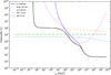 |
Fig. A.1. Energy losses for: Ldisk = 5 × 1044 erg/s, LX = 0.8 × 1044 erg/s, ΓX = 1.95, ϵX,max = 128 keV, rco = 30 rg, rg = 2.35 × 10¹²M7.2 cm, B = 103 G, np = 2 × 109 cm−3. The diffusive escape time is shown for vA = 0.2 c, while the advection time assumes vadv = 0.02 c (as expected for the radial inflow velocity at rco with viscosity parameter α = 0.1). |
To model radiative losses, we consider a disk emission represented by a multicolor black-body Lϵ ∝ ϵ4/3exp(−ϵ/ϵcd) for ϵ > 0.1ϵcd and Lϵ ∝ ϵ3 for ϵ < 0.1ϵcd. The disk cutoff is ϵcd = 31.5 eV. The integrated disk luminosity is Ldisk = 5 × 1044 erg/s. The X-ray emission is a powerlaw Lϵ ∝ ϵ1 − ΓXexp(−ϵ/ϵcX) for ϵ > ϵcd (i.e., above the disk cutoff energy), and Lϵ ∝ ϵ2 below. The X-ray cutoff is set at ϵcX = 128 keV and the integrated luminosity LX = 0.8 × 1044 erg/s.
We assumed a black hole of mass MBH = 107.2 M⊙, and corresponding gravitational radius rg ≃ 2.35 × 10¹²M7.2 cm (Schwarzschild radius rs = 2rg). The Eddington reference luminosity is LEdd = 2 × 1045M7.2 erg/s. We note that for NGC 1068, the all-flavour, integrated (1.5-15 TeV) isotropic-equivalent neutrino luminosity is of order Lν ≃ 1042(d/10 Mpc)2 erg/s ∼LEdd/103, and the estimated bolometric luminosity Lbol ∼ 5 × 1044 erg/s (e.g., IceCube Collaboration 2022; Padovani et al. 2024). We take rco = 30rg for the equatorial extension of the corona. The thermal background proton number density is set to nth = 2 × 109 cm−3, corresponding to a plasma β parameter βp ∼ 1 (we use 1 everywhere). Advective escape (radial inflow) in the corona is parameterized by vadv, where we take vadd = αdvk(rco) as the reference value, with vk(r) the Keplerian velocity field and αd ≃ 0.1 the viscosity parameter.
Figure A.1 shows the energy losses timescales for the given background photon spectral energy distribution. For comparison, for the chosen parameters, the required cosmic-ray power for a NGC 1068 type source is of order LCR ∼ Lν(ctcool/rco)∼(5 − 10)×1043 erg/s, equivalent to an energy density of uCR ≃ LCR/(4πrco2c)∼(3 − 6)×104 erg/cm3 and comparable to the energy density uB ≃ 4 × 10⁴ erg/cm3 of the magnetic field.
All Figures
|
Fig. 1. Proton energy spectra ϵ2 dncor/dϵ (per log-interval of energy) vs. proton energy ϵ predicted by stochastic acceleration in a turbulent corona, starting from mono-energetic protons with a Lorentz factor of γ0 ∼ 1. In each panel, the solid line corresponds to a solution obtained by integrating the Fokker-Planck equation up to time τadv = rco/vadv (model (1) including energy losses, advection, and escape as described in the text), and the dashed line shows the corresponding solution for the same parameters for the generalized Fermi model described by Eq. (5) (model (2)). In all panels, rco is set to 30rg, and in the top and middle panels, vadv ≃ 0.02 c. The upper panel shows the dependence on vA, assuming otherwise a coherence length scale for the turbulence ℓc = 10 rg and an advection velocity vadv = 0.02 c. From left to right, as indicated, vA/c = 0.05, vA/c = 0.10, vA/c = 0.20, and vA/c = 0.40. The middle panel examines the dependence on ℓc, assuming otherwise vA/c = 0.20 and vadv/c = 0.02. From right to left, as indicated, ℓc = 3 rg, ℓc = 10 rg, and ℓc = 30 rg. The bottom panel examines the influence of advection, characterized here by the advection velocity vadv (which sets the advection timescale τadv ≡ rco/vadv), assuming otherwise vA/c = 0.20 and ℓc = 3 rg. From right to left, as indicated, vadv/c = 0.02, vadv/c = 0.05, vadv/c = 0.16 and a (more extreme) case vadv/c = 0.49. The butterfly indicates the range of values needed to reproduce a neutrino spectrum as observed by IceCube for NGC 1068. The energy density spectrum is expressed in units of the background plasma pressure (see Sect. 2.1). In these units, each individual spectrum has been normalized to an integrated fraction of unity for the sake of illustration. |
| In the text | |
|
Fig. 2. Exemplary time-dependent proton energy distribution obtained from jet-shear acceleration with a Fokker-Planck model assuming continuous injection of seed protons with γ0 = 104. As a result of advective escape, the predicted particle spectrum will appear somewhat softer (red, t = τadv, z) compared to the otherwise quasi steady-state distribution (yellow). The gray shaded region illustrates the spectral characteristics required to reproduce the neutrino emission for NGC 1068 as measured by IceCube. |
| In the text | |
|
Fig. 3. Proton energy spectra dup/dlnϵ ≡ ϵ2 dn/dϵ vs. proton energy ϵ for three characteristic scenarios described in the text. For each panel, the energy density distribution is shown in units of the background plasma pressure. Top panel: Stochastic acceleration in the turbulent corona, with a characteristic Alfvénic velocity vA ≃ 0.2 c (see text for details), for model (1) and (2), corresponding to the solid and dashed lines, respectively. Middle panel: Combination of stochastic acceleration in the corona with shear acceleration at the base of the jet (see text for the details of the physical parameters). The stochastic contribution is indicated by dotted lines, the shear contribution by dashed lines, and the sum of the two by solid lines. The different colors correspond to models (1) and (2). For the top and middle panels, the normalization of the energy density in accelerated particles has been fixed in order to reproduce the inferred proton flux. Bottom panel: Modeling of stochastic acceleration, accounting for self-regulation by particle feedback on the turbulence (damping), for a characteristic Alfvén velocity vA ≃ 0.2 c. The plasma β parameter is 0.5 (see Appendix A). |
| In the text | |
|
Fig. A.1. Energy losses for: Ldisk = 5 × 1044 erg/s, LX = 0.8 × 1044 erg/s, ΓX = 1.95, ϵX,max = 128 keV, rco = 30 rg, rg = 2.35 × 10¹²M7.2 cm, B = 103 G, np = 2 × 109 cm−3. The diffusive escape time is shown for vA = 0.2 c, while the advection time assumes vadv = 0.02 c (as expected for the radial inflow velocity at rco with viscosity parameter α = 0.1). |
| In the text | |
Current usage metrics show cumulative count of Article Views (full-text article views including HTML views, PDF and ePub downloads, according to the available data) and Abstracts Views on Vision4Press platform.
Data correspond to usage on the plateform after 2015. The current usage metrics is available 48-96 hours after online publication and is updated daily on week days.
Initial download of the metrics may take a while.