| Issue |
A&A
Volume 691, November 2024
|
|
|---|---|---|
| Article Number | A324 | |
| Number of page(s) | 8 | |
| Section | Astronomical instrumentation | |
| DOI | https://doi.org/10.1051/0004-6361/202451752 | |
| Published online | 22 November 2024 | |
Detecting the near-infrared afterglows of high-redshift gamma-ray bursts using CAGIRE
1
IRAP, Université de Toulouse, CNRS, CNES, UPS,
31401
Toulouse,
France
2
CEA-IRFU, Orme des Merisiers,
91190
Gif-sur-Yvette,
France
3
Aix Marseille Université, CNRS/IN2P3, CPPM,
Marseille,
France
4
LAM, Université Aix-Marseille & CNRS, UMR7326,
38 rue F. Joliot-Curie,
13388
Marseille Cedex 13,
France
5
Instituto de Astronomía, Universidad Nacional Autonoma de México,
Apartado Postal 70-264,
04510
México,
CDMX,
Mexico
★ Corresponding author; francis.fortin@irap.omp.eu
Received:
1
August
2024
Accepted:
21
October
2024
Context. Transient sky astronomy is entering a new era with the advent of the Space Variable Objects Monitor mission (SVOM), successfully launched on 22 June 2024. The primary goal of SVOM is to monitor the hard X-ray sky searching for gamma-ray bursts (GRBs). On top of its on-board follow-up capabilities, SVOM will be backed by its ground segment composed of several facilities, including the near-infrared (NIR) imager CAGIRE. Mounted on the robotic telescope COLIBRI, it will be a unique instrument capable of performing fast follow-up of GRB afterglows in the J and H bands, ideal for capturing high-redshift (z>6) and/or obscured GRBs.
Aims. This paper is aimed at estimating the performances of CAGIRE for GRB NIR afterglow detection based on the characteristics of the detector and the specificities of the COLIBRI telescope. Quickly fading GRB afterglows pose challenges that should be addressed by adapting observing strategies to the capabilities of CAGIRE.
Methods. We used an end-to-end image simulator to produce realistic CAGIRE images, taking into account the results from the characterisation of the ALFA detector used by CAGIRE. We implemented a GRB afterglow generator that simulates infrared light curves and spectra based on published observation of distant GRBs (z>6).
Results. We retrieved the photometry of nine GRB afterglows in various scenarios covered by CAGIRE. Capturing afterglows as early as one minutes after the burst allows for the identification of a NIR counterpart in the brightest four events. When artificially redshifted even further away, these events remain detectable by CAGIRE up to z=9.6 in the J band and z=13.3 in H band, indicating the pioneering potential of CAGIRE in identifying the most distant GRBs to date.
Key words: stars: black holes / gamma-ray burst: general / stars: massive / infrared: general
© The Authors 2024
 Open Access article, published by EDP Sciences, under the terms of the Creative Commons Attribution License (https://creativecommons.org/licenses/by/4.0), which permits unrestricted use, distribution, and reproduction in any medium, provided the original work is properly cited.
This article is published in open access under the Subscribe to Open model. Subscribe to A&A to support open access publication.
1 Introduction
Gamma-ray bursts (GRBs) are high-energy transient events that take place during the evolution of massive stars. They are generally classified according to the duration of the burst (Dezalay et al. 1992; Kouveliotou et al. 1993). Short GRBs (t90<2 s) have been confirmed to originate from the merger of neutron star binaries (BNS, Abbott et al. 2017a), while long GRBs (t90>2 s) have been associated with the collapse of massive stars (MacFadyen & Woosley 1999). Both supernovae (SN, Woosley & Bloom 2006) and kilonovae (KN, Abbott et al. 2017b) events have been associated to GRBs. All GRBs are described by a prompt emission of high-energy photons, followed by an afterglow that quickly fades on the scale of several hours. The prompt emission is produced close to the central engine of the GRB, likely inside the jets outflowing from a newly formed black hole (or magnetar, see e.g. Metzger et al. 2011; 2017). The afterglow comes from the interaction of the jets with the surrounding medium and can radiate from hard X-rays down to radio.
The observation of GRBs provides an ideal window into black hole physics, the accretion-ejection mechanisms that launch relativistic jets, the acceleration of cosmic rays, and into the evolution of massive stars with the association of GRBs to SN as well as BNS gravitational mergers. The intrinsic luminosity of GRBs allows the brightest events to be seen at high redshifts (z > 6); hence, they can be used to probe the conditions of the early universe and constrain the evolution of massive star formation, as well as the composition of the host galaxies or even that of the intergalactic medium. The first generation of stars (population III stars) are also reachable at such redshifts. However, the follow-up study of distant GRB afterglows becomes impossible even with fast-reacting optical observatories past z~6, as radiation below the Lyman α wavelength is progressively shifted out of the optical domain as redshift increases.
The Space Variable Objects Monitor mission (SVOM, Wei et al. 2016) is a space-based GRB observatory with both onboard and ground follow-up capabilities. The main high-energy instrument that is poised to detect prompt GRB emission, called ECLAIRs, will trigger automatic follow-up on the ground segment, which is composed of a collection of small robotic telescopes (GWAC), as well as two 1 m class telescopes, C-GFT, and F-GFT. The latter, also known as COLIBRI (Basa et al. 2022), is a 1.3 m robotic telescope installed in San Pedro Martír observatory, Mexico. It will be capable of observing three different channels simultaneously: two channels with the optical imager DDRAGO (Langarica et al. 2022) operating in the (g, r, i) and (z, y) bands, and one channel with the near-infrared (NIR) imager CAGIRE (Nouvel de la Flèche et al. 2023) operating in the J and H bands. DDRAGO is designed to have its 4k×4k detectors cover a field of view (FoV) of 26′, which will fully cover CAGIRE’s 21.7′ FoV. DDRAGO will be operational by the end of 2024 and once CAGIRE is running (starting summer 2025), the combination of both instruments will make the early sampling of afterglow spectral energy distributions possible over the optical to NIR domain. In turn, this will allow photometric redshifts in the range of z = 3.5–8 to be determined with a 10% level of accuracy (Corre et al. 2018).
Mounted on the Nasmyth focus of COLIBRI, CAGIRE will be able to meet the observational challenges raised by far away and obscured GRBs. The camera is capable of J and H band photometry to probe sources beyond a redshift of 6. Its field of view was designed to cover most (if not all) of the error boxes associated to the localisation of GRBs with ECLAIRs. COLIBRI will allow CAGIRE to begin imaging as soon as one minute after the initial trigger from ECLAIRs (see SVOM System Requirements Document 0702), which is ideal to catch the early times of the fast-decaying afterglow light curves. This combination of COLIBRI’s quick reactivity with CAGIRE’s NIR imaging capabilities is unique in the field of transient sky astronomy.
In this paper, we aim to provide insights into the future capabilities of CAGIRE by analysing its expected performance on already observed distant GRBs detected in the last two decades. We first provide the characteristics of CAGIRE and describe the softwares we used for image simulation and data processing (Sect. 2). We then build a sample of modelled light curves from past GRB afterglows (Sect. 3) that we then feed into the CAGIRE image simulator to test their detectability in various realistic scenarios (Sect. 4). We then discuss these results and present our conclusions in Sects. 5 and 6.
2 CAGIRE: Instrument, image simulation, and signal extraction
2.1 Instrument description and specifications
CAGIRE is a NIR imager that operates in the J (1.22 µm) and H (1.63 µm) bands. The detector is a 2k×2k Astronomical Large Format Array (ALFA) loaned by ESA, sampling the sky at 0.65″/pix, which covers an FoV of 21.7′. The camera is cooled down to operate at 100 K, which allows for a negligible dark current (0.004 e−/s/pix) and for CAGIRE to be sky-limited. The ALFA detector can be read in a non-destructive manner, so that CAGIRE will generate ramps composed of several frames each with a fixed exposure of 1.33 s. The edges of the detector are constituted of a ring of pixels that are not sensitive to light and serve as reference pixels to correct for common mode electronic noise.
2.2 CAGIRE image simulator
We performed simulations of images acquired by CAGIRE at the Nasmyth focus of COLIBRI using the dedicated software described in Nouvel de la Flèche et al. (2023). The simulator was initially based on the software developed by D. Corre (Corre et al. 2018), dedicated to simulating the output images of the COLIBRI telescope. Nouvel de la Flèche et al. (2023) adapted the image simulation and the exposure time calculator to work with CAGIRE and its specificities. The sources within the simulated field of view are taken from the 2MASS catalogue (Cutri et al. 2003) and the sky background added depending on the photometric band. The simulator also includes random cosmic rays hitting the detector during exposures. CAGIRE-specific effects are then applied according to preliminary characterisation of the detector done at CEA and CPPM: the flat-field, dark current, and hot and cold pixels, as well as the persistence of pixels from previous acquisition (in the case they were filled up to at least 80% of their saturation level). Inter-pixel cross-talk and non-linearity from the capacitance effect are added before finally applying the offset level of the detector.
The simulator is able to generate a fading GRB afterglow based on tabulated data included with the software, with light curves sampled at the CAGIRE frequency of ~1.33 s/frame. The base version of this software is publicly available on GitHub1, however, it is no longer maintained.
For this study, we have worked on improving the performances of the CAGIRE image simulator and implementing additional features. Several routines have been parallelised and optimised to be able to generate ramps much quicker, up to an average rate of 2.5 frames per second for longer exposures. The output ramps of the simulator follow the same .FITS data and header formatting as the real instrument. The main addition compared to the base version is the presence of a GRB generator, which uses models of afterglow light curves that are input in the simulator to recreate a fading transient in the final images. It is possible to simulate an afterglow at any time after burst, in both the J and H bands, as well as to change the redshift of the simulated GRB (see more details in Sect. 3). This new version of the CAGIRE image simulator is developed in a private GitLab repository hosted by the Laboratoire d’Astrophysique de Marseille and is mirrored in a public GitHub repository2.
2.3 Observing conditions
As GRBs are unpredictable transients and require a quick followup, COLIBRI will not wait for optimal observing conditions after an alert issued by ECLAIRs. As such, in the rest of the paper, we assume that observations are made in sub-optimal conditions. The seeing at zenith is set to 1″, and the elevation of the targets at 41.8° corresponding to an airmass of 1.5. The Moon’s age is fixed at 7 days after the new moon, although the moon phase has a very slight impact on the sky brightness in J and H bands. The sky brightness in San Pedro Martír is measured to be 17 mag/arcsec2 in J band and 15 mag/arcsec2 in H band (Watson & Corre 2018) normalised for an airmass of 1.5.
2.4 Pre-processing of CAGIRE images
As CAGIRE will operate in up-the-ramp mode, the raw output files consist of a series of frames with increasing signal. The goal of the pre-processing software is to convert the raw ramps into a single image containing the flux in ADU per frame, corrected for instrumental effects, which are ready to be fed into any astrophysical pipeline for data processing (i.e. astrometry, photometry, search for transients). The main tasks of the preprocessing software include the correction of common mode electronic noise and offset of the detector using the ring of reference pixels around the ALFA detector, the creation of differential ramps and their fitting to retrieve the flux for each pixel. The software automatically detects when and where the detector was impacted by a cosmic ray and whether pixels had attained their saturation level during the exposure. The fitting range of the flux was then adjusted accordingly.
A Python version of the pre-processing software is publicly available on the COLIBRI-CAGIRE GitHub collaboration3. It can be used to process both real CAGIRE data and images output from the CAGIRE Image Simulator.
2.5 Photometry extraction
We determined the zero point of the photometry for each simulated image using the stars available in the field of view (N~1000), which are generated along with the GRB afterglow using catalogued magnitudes retrieve through the CDS service Simbad (Wenger et al. 2000). We extracted their flux by performing PSF fitting photometry with the PYTHON/PHOTUTILS package. The fitting of a symmetrical two-dimensional Gaussian PSF was performed in a 15 pixel-wide window around the position of the sources. The background was estimated locally and assumed to be a constant in the fitting window.
The zero points were obtained by fitting the instrumental magnitudes against the catalogued magnitudes. We measured average zero points of ZP J=20.90±0.03 mag and ZPH=21.26±0.04 mag in the observing conditions described in Sect. 2.3. We ensured that the values of the zero points were not affected by the brightness of the stars, as the PSF may deviate from a Gaussian for either very bright or very dim sources.
2.6 Limiting magnitude of CAGIRE
We derived the limiting magnitude at a given signal-to-noise ratio (S/N) of each image using the generic formula that links the magnitude of a given reference star to its measured S/N:
 (1)
(1)
The measurement of the S/N was performed on each reference star with a magnitude between 14 and 16.5, which is the range in brightness where stars do not approach saturation and are still sufficiently bright to extract precise photometry using PSF fitting. The noise from the sky and detector readout is estimated locally in an annulus around each star. We estimated the general detection limit using the median of those measurements.
We present the limiting magnitudes computed for an S/N of 10, 5, and 3 for various exposures in Fig. 1. The typical error on the limiting magnitudes is around 0.05 mag. We worked with individual exposures of 100 s in both bands, since the sky contribution in H band will already fill more than half of the dynamic range of the detector for this integration time. Exposures longer than 100 s are split into 100 s individual exposures taken in a dithering pattern, that is, randomly offset on the sky by 30″. They are are realigned and averaged afterwards. The sky contribution is subtracted using the median of non-aligned images. We note that the drastic evolution of the limiting magnitude between a single 100 s exposure and three 100 s exposures in a dithering pattern is mostly due to the bad subtraction of the background sky and detector defects on the single exposure. The evolution of the limiting magnitude for total exposure times equal or greater than 300 s follows the expected trend (S/N increasing with the square-root of total exposure time), albeit with a shallower slope due to the extra readout noise. This can be partially mitigated as dithering frames increase in number, up to 72 frames of 100 s for a two-hour exposure.
We also explored the possibility of increasing the individual exposure time in J band only, as the sky contribution is much lower than in the H band. We increased the individual J band exposures up to 300 s (225 frames), which is the point at which the pre-processing time becomes longer than the acquisition time. We obtained a detection limit for 3×300 s (900 s total) in the J band at 19.7 (S/N=3), compared to 19.1 for 9×100 s. The increased detection limit is due to the fewer readouts of the detector, as well as the use of a higher number of frames for the fit on the differential ramps, which provides more constrained value for the flux. We note that this advantage towards greater exposures times in J band is mitigated in the case of quickly fading sources such as GRB afterglows, which we discuss in Sect. 4.
We then used the simulated images from CAGIRE to evaluate the detectability of GRB afterglows at high redshift (z>6) in the J and H bands. We first present how we model the afterglow light curves and then explore various observational scenarios depending on the delay between the bursts and the first images, as well as the redshift of the events.
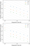 |
Fig. 1 Detection limits of CAGIRE. The exposure times are split into 100 s (75 frames) individual exposures to avoid detector saturation due to the sky background. Grey dashed lines indicate the maximum theoretical evolution of the limiting magnitude (S/N increasing with the square root of the exposure). |
3 Gamma-ray burst database, generating light curves, and spectra
We compiled the modelled infrared light curves of GRB afterglows from the literature for events located at a redshift of 6 and above. We collected a total of nine GRBs with sufficient coverage of their afterglows (see Table 1) to model the evolution of their lightcurve in the observer’s rest frame. The general properties of their prompt emission are presented in Table 2.
The temporal evolution of the light curves is modelled using a decaying broken power law, which (depending on each GRB) may present a break starting from several minutes up to a couple of days after the initial burst alert, and is described by:
![$G(t) = {\left( {{t \over {{t_b}}}} \right)^{ - {\alpha _1}}}{\left[ {{1 \over 2}\left( {1 + {{\left( {{t \over {{t_b}}}} \right)}^{{1 \over \delta }}}} \right)} \right]^{\delta \left( {{\alpha _1} - {\alpha _2}} \right)}},$](/articles/aa/full_html/2024/11/aa51752-24/aa51752-24-eq2.png) (2)
(2)
with α1 and α2 the decay indices before and after the break occurring at tb , and δ a parameter that governs the smoothness of the transition between the two regimes. For the sake of simplicity, we considered the transition to be instantaneous; hence, we fixed δ<<1. Reconstructed lightcurves are shown in Fig. 2.
The spectral shape of the afterglows is considered constant over time and modelled by a power law:
 (3)
(3)
where β is the spectral index. A cut-off is introduced above vLyα=2.47×10¹⁵ Hz, the starting point of the Lyman forest absorption. Between the Lyman α and Lyman β transitions, the loss of flux is calculated according to the relation given in Zuo & Lu (1993), which scales the amount of absorbers with redshift. We note that this is an extrapolation beyond z~4; for reference, according to this model, the loss is of 82% at a redshift of 6 (between 700–850 nm in the observer’s frame) and 98.5% at a redshift of 8 (between 900–1090 nm). Figure 3 provides modelled spectra of GRB 050904A to illustrate this evolution at various redshifts. The flux of the GRB afterglow is thus governed by:
 (4)
(4)
The light curves were normalised using the first measured magnitude in each observation band (listed in Table 1). It was then possible to recover the afterglow light curves in the rest frame of the GRB (Fig. 4). To do this, we take into account the effects of luminosity distance, spectral redshift, and time dilation, with all three following Eqs. (6) and (7) given in Lamb & Reichart (2000). Finally, we applied the same equations backwards to artificially place observed GRBs, as if they were located further away, at higher redshifts.
General information on high-redshift GRBs and model parameters of their NIR afterglow.
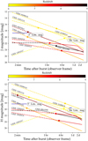 |
Fig. 2 Modelled light curves of GRB afterglows in our sample. Filled circles indicate the first photometric measurement after burst found in the literature; dotted lines indicate extrapolated light curves in J and H bands. Horizontal blue lines indicate the limiting magnitudes achieved in the early-catch (5′ exposures) and late-catch (2 h exposures) scenarios (see Sect. 4). |
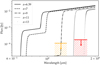 |
Fig. 3 Optical to NIR model spectrum of GRB 050904A at the midpoint of 300 s observations started 1 min after burst. The corresponding CAGIRE detection limits at S/N=3 are shown for the J-band (orange) and H-band (red). |
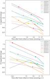 |
Fig. 4 Reconstructed light curves of GRB afterglows in our sample, assuming z=1. Squares indicate the first photometric measurement after burst found in the literature. Dotted lines thus indicate extrapolated light curves in the J and H bands. |
4 Results
4.1 CAGIRE detection in the early-catch scenario
Here, we focus on the detectability of GRBs in the best-case scenario, when CAGIRE is able to start observations exactly one minute after the GRB alert. At such an early time after the burst, the afterglows are fading very quickly. In our case, if an event is already fainter than the detection limit for 3×100 s exposures in each filter, increasing the number of exposures is unlikely to allow CAGIRE to catch up with the decreasing flux of the afterglow. Indeed, the decaying rate in the early-catch scenario is such that the afterglows will typically become dimmer by three to four magnitudes during the first hour (decaying index α ~ 1). In that time, the increase in limiting magnitude is only 0.7 mag.
We also note that in such a case, CAGIRE will likely be the first facility to observe in the NIR. Without prior knowledge of spectrophotometric data coming from other follow-up facilities worldwide, the best course of action is to start the observing blocks with the H band filter. Indeed, while the limiting magnitude in the H band is slightly worse than in the J band, the latter will suffer from the Lyman break at a lower redshifts. By starting observations in the J band, we would lose the advantage of COLIBRI’s fast reacting time for bursts at z>9. Starting early observations in the H band (rather than J) minimises the chances of missing a high-redshift or obscured event. This is in line with CAGIRE’s main science goal of detecting the afterglows of distant and obscured GRBs.
Out of the nine GRBs we simulated, CAGIRE is able to detect GRB 050904A, GRB 090709A, GRB 140515A, and GRB 210905A, with three exposures of 100 s in each band. The nondetected GRBs are located at redshifts >7.8, with the exception of GRB 120521C, which is located at z=6.03. This event is peculiar, however, as the model of its early light curve indicates a rapidly rising source (i.e. the negative exponent in Table 1) before the break at around 8 hr. This results in a very faint source when extrapolating to earlier observation times. However, even if caught at its peak infrared luminosity (J=19.7, H=20.35), it would still be too faint to be reachable by CAGIRE.
Finally, we also computed the S/N reached in the case of CAGIRE, starting observations 2 min after burst instead of 1 min to assess the impact of slight delays in the pointing time at such an early phase of the afterglow. Across our sample, we lost 20% of S/N in the H band and about 8% in the J band. This difference is explained by the H observations taking place earlier, when the decay rate of afterglows are very steep. In this particular case, we cannot detect GRB 090709A in the J band any more, as its S/N passes just below 3.
4.2 CAGIRE detection in the late-catch scenario
In the case a GRB is detected by SVOM/ECLAIRs when the sun is rising in San Pedro Martír, COLIBRI will not be able to point to the target until several hours later, when the sky is dark again. In the worst-case scenario, this would be an average of 12 hours after trigger; of course, any intermediate cases are possible depending on the time of day when the burst happens. In this worst-case scenario, the afterglow magnitude is much fainter than at early times, but the fading rate is also much slower. For typical decay indices of a ~1, the afterglows dim by around 0.1 magnitudes between 12 and 13 hours after the burst; in this case, an afterglow that is less than 0.6 magnitudes below the detection limit for 300 s exposures can be detected by increasing the number of exposures. Hence, the best observing strategy here is to take the deepest images possible, as the increase of S/N with exposure time is potentially able to catch up with the fading afterglows. This is the case for GRB 210905A, for which 2 hr exposures in the late-catch scenario allow us to detect it just above S/N=3 in the J band, when 300 s would not have been enough to pass that threshold.
In the case of the nine listed GRBs in this study, 2 h exposures (72×100 s) are able to reach the magnitude of the two brightest afterglows, GRB 040905A and GRB 210905A. For any other undetected afterglow, such exposures will provide upper limits of J~20 and H~19.5 at three sigma.
However, as discussed in Sect. 2, we can increase the magnitude limit in J band by performing 300 s individual exposures instead of 100 s. This is possible in this late-catch scenario as this does not impede on the H band exposures. The increase in S/N with exposure time is usually faster than the decaying rate of the afterglows. For 24×300 s exposures, we reached a magnitude limit of J=20.47 at S/N=3, which is 0.5 magnitudes deeper than 72×100 s exposures. This translates into a 57% increase in the S/N for J band images. In our list of GRBs, the afterglow of GRB 140515A thus reaches a S/N of 2.7 (instead of 1.7), just below the detection threshold. Hence, in the late-catch scenario, there are key advantages seen when increasing the individual J band exposures from 100 s to 300 s. This will maximise the chances of detecting the GRB counterparts and, at worst, it will give more constraints on the flux’s upper limit.
General properties of the prompt emission of the high-redshift GRBs.
Detectability of GRBs in the proposed scenarios.
4.3 Detecting very high redshift events with CAGIRE
Beyond redshift 6, the impact of luminosity distance on the flux is marginal; it is almost offset by the effect of time dilation since the afterglows are effectively caught at an earlier time after the burst in their rest frame. The main factor governing the loss of flux is the sharp decrease below the Lyman α wavelength. Hence, for intrinsically bright events, CAGIRE is not limited by its specifications nor by the collecting power of COLIBRI, but by the extreme obscuration caused by the Lyman break reaching the J and H photometric bands at high redshifts.
This means that CAGIRE is able to detect bright events such as GRB 050904A, GRB 090709A, GRB 140515A, and GRB 210905A, up to redshifts of 9.6, 8.4, 9.3, and 9.2, respectively, in the J band; along with redshifts of 13.3, 12.6, 12.9, and 12.7, respectively, in the H band at S/N=3 in the early-catch scenario (Table 3). In a late-catch scenario, we are not able to detect the GRBs at significantly greater redshifts, since their detections at their actual redshifts are already marginal. This reinforces the fact that the uniqueness of CAGIRE resides in the combination of a NIR imager with a fast-slewing robotic telescope that is able to work in synergy with SVOM/ECLAIRs as early as two minutes after the burst.
5 Discussion
5.1 Locating GRB afterglows at early times
Locating transient sources within astronomical images necessitates dedicated pipelines, which are yet to be developed for CAGIRE. The S/N of the transient will have an impact on the ability of those pipelines to securely identify it. A S/N greater or equal than 10 should allow for a reliable detection independently of the algorithm used. All of the detected GRBs we simulated fulfil this criteria for the early-catch scenario (except for GRB 090709A in J band) and none of them do so for late-catch scenario. This means that the ability to capture GRB afterglows as early as one minute after the burst is crucial for determining the location of the counterpart to the community and ensuring efficient follow-ups by larger facilities. This is especially important for spectroscopy, where a good level of accuracy is needed to position the slits.
Sampling the early light curves of GRB afterglows also has the intrinsic benefit of probing an epoch rarely observed in the NIR domain. COLIBRI and CAGIRE have the potential to produce a database of early light curves where the evolution of flux may significantly differ from the decaying powerlaw model. This is a caveat that is assumed in our study to extrapolate the reconstructed light curves at times earlier than one hour.
5.2 Lyman alpha flux deficit evolution at high redshifts
The only GRB in our sample that has a magnitude measurement landing within the Lyman forest is GRB 090429B. At a redshift of 9.4, the J band is heavily impacted by the Lyman forest. The model we used to simulate this deficit, given by Zuo & Lu (1993), is based on quasi-stellar objects up to redshift 4. When artificially putting GRB 090429B at a closer distance, this model seems to slightly overestimate the flux loss; for instance, the J band magnitude becomes brighter than the H band. Hence, it is likely that by observing the afterglows of far away GRBs, it will be possible to better constrain the evolution of the effects of Lyman α absorption on a cosmological scale. Along with allowing for a better reconstruction of the intrinsic light curves and spectra of distant GRBs, this would be a way to probe the intergalactic medium and the formation of early galaxies.
5.3 CAGIRE and the general population of GRBs
The main point of this paper is to estimate the performances of CAGIRE in the scope of its scientific goals; namely, the detection of obscured/far away GRB afterglows. However, according to GRBWeb4, 98% of GRBs with an identified redshift lie at z<6 (see Fig. 5 constructed from the data available in GRBWeb). Although the true distribution of GRB redshift is unknown, it is likely that high-redshift GRBs will constitute rare events for CAGIRE. Hence, the camera will follow up on many afterglows that are located closer. Here, we estimate how CAGIRE would fare in this scenario.
We combined two collections of NIR light curves of past GRB afterglows. The first is a compilation by Steve Schulze of composite Rc-band light curves between 1997 and 2013, based on the works of Kann et al. (2006, 2010, 2011); Nicuesa Guelbenzu et al. (2012). It consists of 176 light curves with varying coverage after burst and time sampling. The second compilation is an ongoing project by Damien Turpin (priv. communication) of retrieving photometric measurements of GRB afterglows directly from GCN circulars and the literature. It compiles 2567 NIR photometric measurements in J and H bands on a total of 279 GRB afterglows. So far, the total sample we work with consists of 364 unique afterglows. We also acknowledge the work of Dainotti et al. (2024), who compiled similar data on 535 GRBs, as well as the GRBphot database mentioned in Blažek et al. (2020) and Kann et al. (2024); however, both photometric databases were not available at the time of the data compilation. Since then, GRBphot was released on Vizier and we used it to supplement our database. We found 246 photometric measurements in either the Rc , J, or H bands based on 24 individual bursts. Our database already contained information on 17 of these bursts, meaning we can work with an extra 7 events. Two of them have an insufficient number of datapoints in their light curves for us to use them in our simulations; hence, we have been able to supplement our database with 5 extra GRB light curves, for a total of 369.
The Rc magnitudes are converted to J and H magnitudes using a powerlaw with β=1, which is the average value found in our sample of far away GRBs (although it may vary on across the population of all GRBs). To retrieve the magnitudes of the afterglows at t=1 min (early-catch) and t=12 h (late-catch), we first checked whether there were data points within 10s–20 min (early-catch) and 2 h–5 days (late-catch). If so, we assumed a decay index of α=1; otherwise, we considered the data points to be too far in time to reasonably extrapolate the light curves. So we did not use them in this study.
In the early-catch scenario, we count 142 (150) J band (H band) measurements that we can use. Of them, 12 (13) have an S/N below 3, meaning they are not detected in the J (H) band. Out of the 130 (137) afterglows detected at S/N greater than 3, 111 (118) have a S/N greater than 10 in the J (H) band. This results in an overall detection success rate greater than 90% in the early-catch scenario in both J and H bands.
In the late-catch scenario, we counted 327 (312) J band (H band) measurements that we can use. Of them, 144 (191) have an S/N below 3, meaning they are not detected in the J (H) band. Out of the 183 (121) afterglows detected at S/Ns greater than 3, there are 89 (54) that have a S/N greater than 10 in the J (H) band. This results in an overall detection success rate of 56% in the J and 39% in H bands in the late-catch scenario. Using longer individual exposures (300 s) in the J band provides a slightly better detection success rate of 60% (+13 detections). Again, this is not applicable in the H band as the sky contribution becomes too important past 100 s exposures. We conclude that for a more generic population of GRB afterglows, CAGIRE will be particularly efficient at sampling the early light curves in both the J and H bands and will still serve as a great source of photometric measurements many hours after the bursts occur.
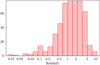 |
Fig. 5 Distribution of measured redshifts in GRBs according to GRBweb. |
5.4 Observatory efficiency
It is difficult to predict the number and nature of GRB afterglows that will effectively be detected by CAGIRE. The population of GRBs observed by SVOM is indeed hard to anticipate because of the low energy threshold of ECLAIRs (helping to detect high- redshift GRBs, Llamas Lanza et al. 2024), fast-reaction time of COLIBRI, and the NIR capabilities of CAGIRE open a new parameter space in transient sky astronomy.
However, we can interpret the detectability numbers we provide in this work (see previous section) in light of known data about the San Pedro Martír observatory site and requirements. According to Carrasco et al. (2012), we can expect an average clear sky fraction greater than 80% at the observatory location. The Functional Performance Requirements document for COLIBRI also specifies that the observatory is expected to be operational 90% of the nights, with the predicted time loss being due to both software and hardware issues. For reference, the contribution from CAGIRE’s hardware problems amounts to 2% (about 7 nights per year). These observational restrictions should not significantly impact the ability of CAGIRE to detect distant and obscured GRB afterglows.
6 Conclusion
Once CAGIRE is operational on the COLIBRI telescope (Q2– Q3 2025), the ground segment of SVOM will have a unique instrument for the follow-up of GRB afterglows. The NIR camera will have the capability of rapid slewing after burst triggers issued from SVOM/ECLAIRs (T−T0 ∼1 min) and identify a counterpart thanks to CAGIRE’s field of view covering ECLAIRs error boxes in a single exposure. We have simulated NIR images output of CAGIRE using an end-to-end simulator in order to realistically assess the performances of the instrument on known GRBs. We modelled the light curves of their afterglows, and produced artificially redshifted events to explore the best capabilities of CAGIRE; out of the nine GRBs with z≥6 with sufficient photometry coverage in the literature to produce lightcurve models, CAGIRE is able to detect the afterglow of the four brightest events. Similar events happening at even higher redshifts can be detected up to z=9.6 (J band) and z=13.3 (H band). It is the combination of the ability to produce images very early after the high-energy triggers with the infrared pushing back the Lyman α break limit that gives CAGIRE the potential to identify counterparts of the farthest GRBs to date (z>9.4). On the general population of GRBs, CAGIRE will perform very well, with the ability to capture more than 90% of afterglow counterparts at early times.
Sampling the early light curves of far away GRBs provides a unique opportunity to probe the very first instants of their afterglows thanks to time dilation effects. Less than 20% of the GRBs in our sample have photometry available at times earlier than 2 minutes in the NIR, most of which are reconstructed from multi-band data. These early epochs are likely to differ from a typical decaying powerlaw and CAGIRE will be capable of systematically providing early photometry to constrain their evolution.
Beyond a redshift of 6, CAGIRE will also be able to see GRBs issued from population III massive stars that initiated the reionisation epoch. This may help in resolving the bias between star formation rates inferred by the currently observed occurrence of GRBs (Wang 2013) and the models using the interstellar medium (ISM) properties of high-redshift galaxies (see e.g. Markov et al. 2022). The evolution in the composition of the intergalactic medium can also be probed through the shape of the Lyman forest, allowing us to put observational constraints on cosmological parameters (Sarkar et al. 2021). Thus, the potential scientific results brought by CAGIRE in the scope of the SVOM mission reach many domains of astrophysics, especially once COLIBRI, as an observatory independently of SVOM, becomes available for the wider community of astronomers.
Acknowledgements
F. Fortin is grateful for the funding from CNES. We thank Lynred, ESA and the LabEx FOCUS for making the ALFA detector available for CAGIRE. We also thank Steve Schulze for making their database public on GitHub (https://github.com/steveschulze/kann_optical_afterglows).
References
- Abbott, B. P., Abbott, R., Abbott, T. D., et al. 2017a, ApJ, 848, L13 [CrossRef] [Google Scholar]
- Abbott, B. P., Abbott, R., Abbott, T. D., et al. 2017b, ApJ, 848, L12 [Google Scholar]
- Basa, S., Lee, W. H., Dolon, F., et al. 2022, in SPIE Conference Series, 12182, Ground-based and Airborne Telescopes IX [Google Scholar]
- Blažek, M., de Ugarte Postigo, A., Kann, D. A., et al. 2020, in SPIE Conference Series, 11452, Software and Cyberinfrastructure for Astronomy VI [Google Scholar]
- Carrasco, E., Carramiñana, A., Sánchez, L. J., Avila, R., & Cruz-González, I. 2012, MNRAS, 420, 1273 [NASA ADS] [CrossRef] [Google Scholar]
- Cenko, S. B., Butler, N. R., Ofek, E. O., et al. 2010, AJ, 140, 224 [NASA ADS] [CrossRef] [Google Scholar]
- Chrimes, A. A., Levan, A. J., Stanway, E. R., et al. 2019, MNRAS, 488, 902 [NASA ADS] [CrossRef] [Google Scholar]
- Corre, D., Basa, S., Klotz, A., et al. 2018, in SPIE Conference Series, 10705, Modeling, Systems Engineering, and Project Management for Astronomy VIII [Google Scholar]
- Cucchiara, A., Levan, A. J., Fox, D. B., et al. 2011, ApJ, 736, 7 [Google Scholar]
- Cutri, R. M., Skrutskie, M. F., van Dyk, S., et al. 2003, VizieR Online Data Catalog: 2MASS All-Sky Catalog of Point Sources [Google Scholar]
- Dainotti, M. G., De Simone, B., Mohideen Malik, R. F., et al. 2024, MNRAS, 533, 4023 [NASA ADS] [CrossRef] [Google Scholar]
- Dezalay, J. P., Barat, C., Talon, R., et al. 1992, in American Institute of Physics Conference Series, 265, 304 [NASA ADS] [Google Scholar]
- Greiner, J., Krühler, T., Fynbo, J. P. U., et al. 2009, ApJ, 693, 1610 [NASA ADS] [CrossRef] [Google Scholar]
- Haislip, J. B., Nysewander, M. C., Reichart, D. E., et al. 2006, Nature, 440, 181 [NASA ADS] [CrossRef] [Google Scholar]
- Kann, D. A., Klose, S., & Zeh, A. 2006, ApJ, 641, 993 [NASA ADS] [CrossRef] [Google Scholar]
- Kann, D. A., Klose, S., Zhang, B., et al. 2010, ApJ, 720, 1513 [Google Scholar]
- Kann, D. A., Klose, S., Zhang, B., et al. 2011, ApJ, 734, 96 [NASA ADS] [CrossRef] [Google Scholar]
- Kann, D. A., White, N. E., Ghirlanda, G., et al. 2024, A&A, 686, A56 [NASA ADS] [CrossRef] [EDP Sciences] [Google Scholar]
- Kouveliotou, C., Meegan, C. A., Fishman, G. J., et al. 1993, ApJ, 413, L101 [NASA ADS] [CrossRef] [Google Scholar]
- Lamb, D. Q., & Reichart, D. E. 2000, ApJ, 536, 1 [Google Scholar]
- Langarica, R., Watson, A. M., Angeles, F., et al. 2022, in SPIE Conference Series, 12184, Ground-based and Airborne Instrumentation for Astronomy IX [Google Scholar]
- Laskar, T., Berger, E., Tanvir, N., et al. 2014, ApJ, 781 arXiv e-prints [arXiv:1307.6586] [Google Scholar]
- Llamas Lanza, M., Godet, O., Arcier, B., et al. 2024, A&A, 685, A163 [NASA ADS] [CrossRef] [EDP Sciences] [Google Scholar]
- MacFadyen, A. I., & Woosley, S. E. 1999, ApJ, 524, 262 [NASA ADS] [CrossRef] [Google Scholar]
- Markov, V., Carniani, S., Vallini, L., et al. 2022, A&A, 663, A172 [NASA ADS] [CrossRef] [EDP Sciences] [Google Scholar]
- Markwardt, C. B., Barthelmy, S. D., Baumgartner, W. H., et al. 2012a, GCN, 13333 [Google Scholar]
- Markwardt, C. B., Barthelmy, S. D., Baumgartner, W. H., et al. 2012b, GCN, 13807 [Google Scholar]
- Melandri, A., Bernardini, M. G., D’Avanzo, P., et al. 2015, A&A, 581, A86 [NASA ADS] [CrossRef] [EDP Sciences] [Google Scholar]
- Metzger, B. D., Giannios, D., Thompson, T. A., Bucciantini, N., & Quataert, E. 2011, MNRAS, 413, 2031 [Google Scholar]
- Metzger, B. D., Berger, E., & Margalit, B. 2017, ApJ, 841, 14 [NASA ADS] [CrossRef] [Google Scholar]
- Nicuesa Guelbenzu, A., Klose, S., Greiner, J., et al. 2012, A&A, 548, A101 [NASA ADS] [CrossRef] [EDP Sciences] [Google Scholar]
- Nouvel de la Flèche, A., Atteia, J.-L., Boy, J., et al. 2023, Exp. Astron., 56, 645 [CrossRef] [Google Scholar]
- Ohno, M., Iwakiri, W., Suzuki, M., et al. 2009, GCN, 9653 [Google Scholar]
- Rossi, A., Frederiks, D. D., Kann, D. A., et al. 2022, A&A, 665, A125 [NASA ADS] [CrossRef] [EDP Sciences] [Google Scholar]
- Sakamoto, T., Barbier, L., Barthelmy, S., et al. 2005, GCN, 3938 [Google Scholar]
- Sakamoto, T., Barthelmy, S. D., Baumgartner, W. H., et al. 2009, GCN, 9640 [Google Scholar]
- Sakamoto, T., Barthelmy, S. D., Baumgartner, W. H., et al. 2010, GCN, 10371 [Google Scholar]
- Sarkar, A. K., Pandey, K. L., & Sethi, S. K. 2021, J. Cosmology Astropart. Phys., 2021, 077 [CrossRef] [Google Scholar]
- Stamatikos, M., Barthelmy, S. D., Baumgartner, W. H., et al. 2009, GCN, 9290 [Google Scholar]
- Stamatikos, M., Barthelmy, S. D., Baumgartner, W. H., et al. 2014, GCN, 16284 [Google Scholar]
- Tagliaferri, G., Antonelli, L. A., Chincarini, G., et al. 2005, A&A, 443, L1 [NASA ADS] [CrossRef] [EDP Sciences] [Google Scholar]
- Tanvir, N. R., Laskar, T., Levan, A. J., et al. 2018, ApJ, 865, 107 [NASA ADS] [CrossRef] [Google Scholar]
- Wang, F. Y. 2013, A&A, 556, A90 [NASA ADS] [CrossRef] [EDP Sciences] [Google Scholar]
- Watson, A. M., & Corre, D. 2018, COLIBRÍ Expected Performance, Tech. Rep. No. GFT-AN-A3135-046-UNAM, UNAM [Google Scholar]
- Wei, J., Cordier, B., Antier, S., et al. 2016, arXiv e-prints [arXiv:1610.06892] [Google Scholar]
- Wenger, M., Ochsenbein, F., Egret, D., et al. 2000, A&AS, 143, 9 [NASA ADS] [CrossRef] [EDP Sciences] [Google Scholar]
- Woosley, S. E., & Bloom, J. S. 2006, ARA&A, 44, 507 [Google Scholar]
- Zuo, L., & Lu, L. 1993, ApJ, 418, 601 [NASA ADS] [CrossRef] [Google Scholar]
All Tables
General information on high-redshift GRBs and model parameters of their NIR afterglow.
All Figures
|
Fig. 1 Detection limits of CAGIRE. The exposure times are split into 100 s (75 frames) individual exposures to avoid detector saturation due to the sky background. Grey dashed lines indicate the maximum theoretical evolution of the limiting magnitude (S/N increasing with the square root of the exposure). |
| In the text | |
|
Fig. 2 Modelled light curves of GRB afterglows in our sample. Filled circles indicate the first photometric measurement after burst found in the literature; dotted lines indicate extrapolated light curves in J and H bands. Horizontal blue lines indicate the limiting magnitudes achieved in the early-catch (5′ exposures) and late-catch (2 h exposures) scenarios (see Sect. 4). |
| In the text | |
|
Fig. 3 Optical to NIR model spectrum of GRB 050904A at the midpoint of 300 s observations started 1 min after burst. The corresponding CAGIRE detection limits at S/N=3 are shown for the J-band (orange) and H-band (red). |
| In the text | |
|
Fig. 4 Reconstructed light curves of GRB afterglows in our sample, assuming z=1. Squares indicate the first photometric measurement after burst found in the literature. Dotted lines thus indicate extrapolated light curves in the J and H bands. |
| In the text | |
|
Fig. 5 Distribution of measured redshifts in GRBs according to GRBweb. |
| In the text | |
Current usage metrics show cumulative count of Article Views (full-text article views including HTML views, PDF and ePub downloads, according to the available data) and Abstracts Views on Vision4Press platform.
Data correspond to usage on the plateform after 2015. The current usage metrics is available 48-96 hours after online publication and is updated daily on week days.
Initial download of the metrics may take a while.