| Issue |
A&A
Volume 691, November 2024
|
|
|---|---|---|
| Article Number | A349 | |
| Number of page(s) | 19 | |
| Section | Astrophysical processes | |
| DOI | https://doi.org/10.1051/0004-6361/202451097 | |
| Published online | 25 November 2024 | |
The Galactic population of canonical pulsars
II. Taking into account several evolutionary paths: Interstellar medium interaction, Galactic potential, and a death valley
1
Université de Strasbourg, CNRS, Observatoire Astronomique de Strasbourg, UMR 7550, 67000 Strasbourg, France
2
National Centre for Radio Astrophysics, Tata Institute for Fundamental Research, Post Bag 3, Ganeshkhind, Pune 411007, India
3
Janusz Gil Institute of Astronomy, University of Zielona Góra, ul. Szafrana 2, 65-516 Zielona, Góra, Poland
⋆ Corresponding author; This email address is being protected from spambots. You need JavaScript enabled to view it.
Received:
13
June
2024
Accepted:
16
October
2024
Abstract
Context. Pulsars are highly magnetised rotating neutron stars, emitting in a broad electromagnetic energy range. These objects were discovered more than 55 years ago and are astrophysical laboratories for studying physics at extreme conditions. Reproducing the observed pulsar population helps refine our understanding of their formation and evolution scenarios, as well as their radiation processes and geometry.
Aims. In this paper, we improve our previous population synthesis by focusing on both the radio and γ-ray pulsar populations, investigating the impact of the Galactic gravitational potential and of the radio emission death line. To elucidate the necessity of a death line, we implemented our refined initial distributions of the spin period and spacial position at birth. This approach allowed us to elevate the sophistication of our simulations to the most recent state-of-the-art approaches.
Methods. The motion of each individual pulsar was tracked in the Galactic potential by a fourth-order symplectic integration scheme. Our pulsar population synthesis took into account the secular evolution of the force-free magnetosphere and magnetic field decay simultaneously and self-consistently. Each pulsar was evolved from birth to the present time. The radio and γ-ray emission locations were modelled by the polar cap geometry and striped wind model, respectively.
Results. By simulating ten million pulsars, we found that including a death line allows us to better reproduce the observational trend. However, when simulating one million pulsars, we obtained an even more realistic P−Ṗ diagram, whether or not a death line was included. This suggests that the ages of the detected pulsars might be overestimated and so, it sets the need for a death line in pulsar population studies into question. Kolmogorov-Smirnov tests confirm the statistical similarity between the observed and simulated P−Ṗ diagram. Additionally, simulations with increased γ-ray telescope sensitivities hint at a significant contribution coming from the γ-ray pulsars to the GeV excess in the Galactic centre.
Key words: gravitation / methods: statistical / pulsars: general / gamma rays: stars / radio continuum: stars
© The Authors 2024
 Open Access article, published by EDP Sciences, under the terms of the Creative Commons Attribution License (https://creativecommons.org/licenses/by/4.0), which permits unrestricted use, distribution, and reproduction in any medium, provided the original work is properly cited.
This article is published in open access under the Subscribe to Open model. This email address is being protected from spambots. You need JavaScript enabled to view it. to support open access publication.
1. Introduction
Pulsars, discovered by Jocelyn Bell Burnell in 1967 (Hewish et al. 1969), are rotating neutron stars born in a core-collapse supernova. They are highly magnetised and surrounded by a plasma-filled magnetosphere emitting regular pulses of radiation at their spin frequency. Due to the magneto-dipole losses, they lose rotational kinetic energy and their spin period increases. Extensive radio surveys have been performed, for instance, by the Parkes and Arecibo radio-telescopes, with 3700 pulsars discovered thus far (Manchester et al. 2005). In Table 1, we list the canonical pulsar population defined by isolated pulsars with periods longer than 20 ms that are not magnetars. Although pulsars were first observed in radio, they were later found to be also bright in X-rays, optical, and γ-rays. Large Area Telescope (LAT) on board the Fermi satellite, has discovered dozens of radio-quiet γ-ray pulsars as well as millisecond pulsars (MSPs). Since its launch, the LAT has detected about 300 pulsars (Abdo et al. 2013; Smith et al. 2019, 2023) and unveiled a new perspective, expanding our understanding about pulsar emission mechanisms by increasing the sample of neutron stars detectable through their high energy emission. Moreover, the distinct radiation process involved in high-energy photon production and its unique beaming properties offer an alternative viewpoint on the global pulsar population.
Number of known canonical pulsars, with spin-down luminosity, Ė, above and below 1028 W, and above 1031 W.
With the advent of future surveys such as Square Kilometre Array (SKA1) or Cherenkov Telescope Array (CTA2), many more pulsars will be detected in both these wavelengths. Those instruments are scheduled to start collecting data by the end of the decade. SKA is going to be 50 times more sensitive than current telescopes and will survey the sky 10 000 times faster than any existing imaging radio telescope (McMullin et al. 2020). CTA is aimed at detecting γ-rays in the energy range from a few tens of GeV up to hundreds of TeV (Hofmann & Zanin 2023), while Fermi/LAT operates in the energy range from 20 MeV to several hundred GeV3 and the High Energy Stereoscopic System (HESS) operates in the energy range from 0.03 to 100 TeV4.
Pulsar population synthesis (PPS) is a powerful tool for predicting the discovery rate of new pulsars to better understand their emission processes and to constrain their overall properties. In a PPS, pulsars are generated from their birth and evolved up to the present time. Once the sample of pulsars is generated, detection criteria can be applied to check whether they can be detected by current and future telescopes. The detectability of an individual pulsar in a given energy band, radio, or γ-ray depends on whether the associated emission beam intersects our line of sight and on the sensitivity of the corresponding instrument.
Most PPS studies assume that neutron stars are rotating in vacuum (Faucher-Giguère & Kaspi 2006; Popov et al. 2010; Johnston et al. 2020) or take only radio or γ-ray emission into account separately (Watters & Romani 2011; Gullón et al. 2014), or assume a constant magnetic field during the evolution process (Gonthier et al. 2002; Faucher-Giguère & Kaspi 2006; Johnston & Karastergiou 2017). Dirson et al. (2022) modelled, for the first time, the population of both the γ-ray and radio pulsars, taking into account the state-of-the-art force-free magnetosphere model in conjunction with a prescription for the magnetic field decay. The neutron star radiation is produced by relativistic charged particles flowing within their magnetosphere. Therefore, the plasma back reaction must be taken into account in the evolution of the pulsar period and magnetic inclination angle. While the location of the γ-ray emission site is still under debate, different regions have been suggested. These are, for instance, the polar cap region (Sturrock 1971; Ruderman & Sutherland 1975; Daugherty & Harding 1982, 1996) at low altitudes, the slot gap along the last open magnetic field lines (Arons 1983; Muslimov & Harding 2004; Harding et al. 2008; Harding & Muslimov 2011), or the outer gaps at high altitudes within the light-cylinder, in the outer magnetosphere (Cheng et al. 1986; Hirotani 2008; Takata et al. 2011). Emission is also possible outside the light cylinder, in the so-called striped wind (Pétri 2009, 2011), which was used for the first time by Dirson et al. (2022) in a PPS study. The radio emission is described as usual by the polar cap model. In this work, as in Dirson et al. (2022), we reproduce only the canonical pulsar population in our Galaxy.
While the study by Dirson et al. (2022) yielded satisfactory results when simulating a population closely resembling the observed pulsar population in the P−Ṗ diagram, there was room for improvement regarding the pulsar trajectories within the Milky Way. Specifically, the Dirson et al. (2022) study was limited by the assumption that pulsars move in a ballistic motion depicted by straight lines at a constant speed from their birth to the present time. A noticeable discrepancy arises when comparing the observed position of pulsars to the predictions, revealing a significant disparity in both spatial distributions.
Dirson et al. (2022) did not require a death line to reproduce the P−Ṗ diagram; thus, it was not implemented in their PPS. However the death line segregates neutron stars generating particles through pair cascading from those not radiating any more because of the quenching of this pair avalanche; hence, they are called dead pulsars. The effect of the death line assumption on the PPS differs from the PPS performed by Graber et al. (2024), where the authors did not consider a death line and instead relied only on as special radio luminosity law to eliminate some pulsars in the P−Ṗ diagram.
In this paper, we further improve the PPS of Dirson et al. (2022) by examining the necessity of a death line to explain the observed canonical pulsar population and discuss the γ-ray pulsar population in depth. Moreover, our study helps to better understand the impact of changing the parameters of our model as well as their physically meaningful ranges. The paper is organised as follows. In Sect. 2, we detail our PPS model, recalling the processes for generation and evolution of the pulsar sample, as well as the description of the Galactic potential and the death line, discussing our adopted multi-wavelength detection criteria. The results are shown in Sect. 3 and discussed in Sect. 4, followed by a summary in Sect. 5.
2. Description of the PPS model
Our PPS study is based on a self-consistent state-of-the-art evolution of the neutron star geometry of radio and γ-ray emission, magnetic field, and proper motion within the Milky Way. In this section, we detail our model by exposing, first, the generation of individual pulsars, their initial position, magnetic field, and spin period; second, we considered how these quantities evolve in time. We also give explicit expressions for the Galactic potential used in our simulations and introduce the death line before discussing the radio and γ-ray detection criteria. We stress that the model parameters used in this section have been carefully chosen by comparing simulated data with actual observations, varying the unknown input parameters in sensible physical ranges (see Appendix C for more details).
2.1. Generation of pulsars
We generated a population of pulsars whose real ages are selected in ascending order, for example, every X years if the birth rate is 1/X yr−1, with their age being between 0 yr and the age of the Milky Way at maximum. The age of the Milky Way does not significantly differ from the age of the Universe estimated about tH ≈ 13.8 × 10⁹ yr, therefore, a total number of tH/X pulsars ought to be simulated. The best value for this birth rate was found to be 1/41 yr−1, see Appendix C. Our value is consistent with earlier investigations by Faucher-Giguère & Kaspi (2006), Gullón et al. (2014), Johnston & Karastergiou (2017), where the authors evaluated the birth rate of pulsars to be in the range [1/150, 1/33] yr−1. With X = 41 yr we should generate more than 107 pulsars, however, we chose to emulate only 107 pulsars in a first run and 106 in a second run for the following two reasons. First, the computation time is significantly decreased, secondly pulsars older than 107 yr are generally not detected. This approach was also chosen because it allows us to verify whether our birth rate is realistic, by comparing our results from the simulation to the observations. Our approach is different from previous works such as Gullón et al. (2014) and Johnston & Karastergiou (2017), where they stopped the simulation whenever their detected number of pulsars would equal the number of observed pulsars.
To describe the position of the pulsars in the Galaxy, we use the right-handed Galacto-centric coordinate system (x, y, z) with the Galactic centre at its origin, y increasing in the disc plane towards the location of the Sun, and z increasing towards the direction of the north Galactic pole. The initial spatial distribution of the pulsars is given by Paczynski (1990). He found two distributions, one describing the radial spread and one the spread in altitude, however only his distribution in altitude is used in our work because the radial distribution in the galactic plane is better depicted in Yusifov & Küçük (2004) by the Milky Way’s pulsar surface density, defined as
 (1a)
(1a)
 (1b)
(1b)
where R is the axial distance from the z-axis, and z is the distance from the Galactic disc. The numerical values for the constants are, A = 37.6 kpc−2, a = 1.64, b = 4.0, R1 = 0.55 kpc, hc = 180 pc, and R⊙ = 8.5 kpc. These values are in agreement with the distribution of young massive stars in our galaxy (Li et al. 2019). The purpose of choosing Eq. (1a) to describe the radial spread is to put neutron stars birth positions within the spiral arms of the Galaxy. More precisely, the Galactic spiral structure contains four arms with a logarithmic shape function, allowing us to obtain the azimuthal coordinate ϕ as a function of the distance from the Galactic center:
 (2)
(2)
The values of the models describing each arm are given in Table 2. These values were used by Ronchi et al. (2021) and taken from Yao et al. (2017) to match the shape of the arms of the Galaxy. The local arm is not modeled because of its very low density, much smaller than the four other arms. Each star has an equal probability to be in one of the four arms, its angular coordinate, ϕ, for a given R being deduced from (1a). Furthermore, the Galaxy is not static, and its arms are moving with an approximated period T = 250 Myr (Skowron et al. 2019). Since we also know that the Galaxy is rotating in the clockwise direction, by knowing the age of a pulsar we can know its angular position at birth. Following the same procedures as Ronchi et al. (2021), to avoid artificial features near the Galactic center, noise is added to both coordinates R and ϕ. For instance ϕcorr = ϕrand exp(−0.35 R), where ϕrand is randomly drawn from a uniform distribution between 0 and 2 π. Then, rcorr will be taken from a normal distribution with a mean of 0 and a standard deviation, σcorr = 0.07 R, and we add these two corrections to ϕ and R, respectively. Therefore, Rbirth = R + rcorr and  , where tage is the age of the pulsar. As soon as Rbirth and ϕbirth are known, we can convert these coordinates in x and y Galacto-centric coordinates for each pulsar.
Parameters of the Milky Way Spiral Arm structure.
Next, we need to describe the individual properties of each pulsar, namely, its inclination angle α, which is the angle between its rotation axis and its magnetic axis, its initial spin period, P0, and initial magnetic field, B0, at birth. The inclination angle, α, is assumed to follow an isotropic distribution generated from a uniform distribution U ∈ [0, 1] and given by α = arccos(2 U − 1). In our work, the initial spin period and magnetic field follow both a log-normal distribution, as suggested from the results of a study of 56 young neutron stars by Igoshev et al. (2022), while other works simply use a Gaussian distribution for the spin period at birth (Faucher-Giguère & Kaspi 2006; Gullón et al. 2014; Johnston et al. 2020); whereas for the magnetic field, the prescription is the same as ours. Explicitly, the probability distributions for an initial magnetic field B0 and an initial period P0 are given by:
 (3)
(3)
 (4)
(4)
The distribution for the magnetic field is identical to the one used in other pulsar population synthesis like for instance Faucher-Giguère & Kaspi (2006), Gullón et al. (2014), Johnston et al. (2020), Yadigaroglu & Romani (1995), and Watters & Romani (2011).
According to Hobbs et al. (2005) a Maxwellian distribution for the kick velocity at birth best replicates the observations and is given by
 (5)
(5)
The mean velocity of the distribution is related to the standard deviation by  , with a standard deviation σv = 265 km/s for pulsars. The velocity value drawn from the Maxwellian distribution is then distributed along the unit vector of the rotation axis, which is generated, as detailed in Sect. 2.5. Moreover compared to the study of Dirson et al. (2022), we introduce a novelty; namely, the alignment between the kick velocities at birth and the rotation axis of the pulsar, as suggested by Rankin (2007).
2.2. Pulsar evolution
The pulsar initial period, P0, inclination angle, α0, and magnetic field, B0, are evolved in time in a fully self-consistent way taking into account the spin-down losses and the internal magnetic field dissipation within the neutron star. The neutron star period is evolved according to the force-free magnetosphere model, which takes into account the electric current and charge flowing inside the magnetosphere. The spin-down luminosity, Ė, is
 (6)
(6)
 (7)
(7)
where I is the neutron star moment of inertia approximately equal to I ≈ 1038 kg m2, Ω = 2π/P the rotation frequency of the pulsar (P is the spin period),  its time derivative, and R = 12 km the typical radius of a neutron star, as found by recent NICER observations (Riley et al. 2019; Bogdanov et al. 2019). Then, B is the magnetic field at the magnetic equator, α the inclination angle, μ0 the vacuum permeability constant, μ0 = 4π × 10−7 H/m, and c the speed of light. The term Lffe for the spin-down luminosity was given by Spitkovsky (2006) and Pétri (2012). Equation (6) clearly shows the correlation between the obliquity, the magnetic field and the rotation frequency. Combining Eqs. (6) and (7) leads to
 (8)
(8)
 (9)
(9)
which is written in a more concise form where n is the braking index, its value being n = 3 for magnetic dipole radiation.
The integral of motion between Ω and α is also very useful and is expressed as
 (10)
(10)
where the quantities with a subscript of 0 indicate their initial value. Those without a subscript display their current value at present time.
As shown by Gullón et al. (2014) a decaying magnetic field better accounts for comparison between pulsar population synthesis and observations. Therefore, we prescribe a magnetic field decay according to a power law
 (11)
(11)
where αd is a constant parameter controlling the rate of the magnetic field decay and τd the typical decay timescale, which depends on the initial magnetic field as demonstrated by magneto-thermal evolution models (Viganò et al. 2013). We took these results into account by defining the decay timescale, τ1, for a magnetic field strength, B1, such that τ1 B1αd = τd B0αd. Thus, τ1 is another magnetic field decay time scale, corresponding to a certain magnetic field value, B1. Three different τ1 values are considered in this work, randomly chosen for each pulsar generated: 1.5 × 10⁵ yr or 3.5 × 10⁵ yr or 2.5 × 10⁶ yr. Each of these timescales corresponds to a magnetic field value, B1, of 1 × 10⁸ T, 3 × 10⁸ T, and 2 × 10⁹ T. Then the probabilities to get these values of τ1 and B1 to be adopted for one pulsar are 0.23, 0.46 and 0.31, respectively. These three probabilities actually approximate the probability density function for τ1 and B1, and were already sufficient to reproduce the canonical population. Finding the complete distribution for τ1 and B1 would require further investigations not needed in our study. Moreover, the distributions of τ1 and B1 would physically represent the whole ensemble of trajectories possible in the P−Ṗ diagram for canonical pulsars as in Fig. 10 of Viganò et al. (2013). Therefore, each pulsar has three possible evolutionary paths in the simulation, which is an empirical way of reproducing the P−Ṗ diagram in a better way than having only one evolutionary path. These particular choices for the discrete values were only guided by trial and error. The value of αd can be found in Table 5 of Sect. 3.
In line with the spin-down luminosity, the inclination angle satisfies another evolution equation, which (after integration) was found by Philippov et al. (2014) for a spherically symmetric neutron star with a constant magnetic field. With our decaying prescription the inclination angle α is found by solving
![Mathematical equation: $$ \begin{aligned} \ln (\sin \alpha _0)&+ \frac{1}{2\sin ^{2}\alpha _0} + K \Omega _{0}^{2} \frac{\cos ^{4}\alpha _{0}}{\sin ^{2}\alpha _{0}} \frac{\alpha _{d} \tau _{\rm d} B_{0}^{2}}{\alpha _{\rm d} - 2}\! \left[\left(1+\frac{t}{\tau _{\rm d}}\right)^{1-2/\alpha _{\rm d}}-1\!\right]\nonumber \\&\qquad = \ln (\sin \alpha ) + \frac{1}{2\sin ^2\alpha }, \end{aligned} $$](/articles/aa/full_html/2024/11/aa51097-24/aa51097-24-eq16.gif) (12)
(12)
where t is the time representing the age of the pulsar and K = R6/I c3. The typical decay timescale for a mean magnetic field of 2.5 × 10⁸ T is 4.6 × 10⁵ yr in Viganò (2013); however, in this study, the typical decay timescale associated to this magnetic field is 3.5 × 10⁵ yr. This result is is very close to the estimate of Viganò (2013) for the same field strength.
2.3. Description of the Galactic potential
Finally, we need to follow the particle motion within the Galactic potential. Each pulsar evolves in the gravitational potential Φ subject to an acceleration  according to
 (13)
(13)
Equation (13) is integrated numerically thanks to a position-extended Forest Ruth-like (PEFRL) algorithm (Forest & Ruth 1990), a fourth-order integration scheme, presented in Appendix A, with a convergence and accuracy study. We now discuss the galactic potential model used.
The Galaxy is divided in four distinct regions with different mass distributions and associated gravitational potentials. The four potentials are: the bulge, Φb, the disk, Φd, the dark matter halo, Φh, and the nucleus, Φn. The total potential of the Milky Way Φtot is the sum of these potentials
 (14)
(14)
The expressions for these potentials are taken from Bajkova & Bobylev (2021) with parameters given in Table 3. The nucleus mass was found in Bovy (2015).
Constants values used for the different potentials.
The potential for the bulge Φb and for the disk Φd were both chosen to have the form proposed by Miyamoto & Nagai (1975), which are typically used for models of the gravitational potential of the Milky Way. They are expressed as:
![Mathematical equation: $$ \begin{aligned} \Phi _i(R,z) = -\frac{GM_i}{\left[R^2+\left(a_i+\sqrt{z^2+b_i^2}\right)^2\right]^{1/2}}, \end{aligned} $$](/articles/aa/full_html/2024/11/aa51097-24/aa51097-24-eq20.gif) (15)
(15)
where R2 = x2 + y2, and i = b is for the bulge and i = d is for the disk. In those formula, R, depends on the coordinates x and y, while ai and bi are the scale parameters of the components in kpc, Mi is the mass (for the disk or the bulge), and G is the gravitational constant. The constant values can be found in Table 3.
Solving the pulsar equation of motion requires to compute the gradient of the potentials, the derivatives of the disk and the bulge potentials are:
![Mathematical equation: $$ \begin{aligned} \frac{\partial \Phi _i}{\partial x_j}&= \frac{G M_i x_j}{\left[R^2+\left(a_i+\sqrt{z^2+b_i^2}\right)^2\right]^{3/2}},\end{aligned} $$](/articles/aa/full_html/2024/11/aa51097-24/aa51097-24-eq21.gif) (16)
(16)
![Mathematical equation: $$ \begin{aligned} \frac{\partial \Phi _i}{\partial z}&= \frac{G M_i z\left(a_i+\left(z^2+b_i^2\right)^{\frac{1}{2}}\right)}{\left[R^2+\left(a_i+\sqrt{z^2+b_i^2}\right)^2\right]^{3/2} \ \left(z^2+b_i^2\right)^{1/2}}, \end{aligned} $$](/articles/aa/full_html/2024/11/aa51097-24/aa51097-24-eq22.gif) (17)
(17)
xj being either x or y. Equation (16) is the derivative for the potential of Miyamoto Nagai, where i = d or i = b depending on disk or bulge derivative. Equation (17) is the derivative of the Miyamoto Nagai potential with respect to the z coordinate.
The potential for the dark matter halo Φh, according to the frequently used potential of Navarro et al. (1997), is expressed as
 (18)
(18)
where Mh is the mass of the halo, r = x2 + y2 + z2, and ah is the length scale whose values are found in Table 3. The derivative of Eq. (18) with respect to any coordinate xj (x, y, z) is:
![Mathematical equation: $$ \begin{aligned} \frac{\partial \Phi _{\rm h}}{\partial x_j} = \frac{G M_{\rm h} x_j}{r^2} \ \left[\frac{1}{r} \ \ln \left(1+\frac{r}{a_{\rm h}}\right) - \frac{1}{r+a_{\rm h}}\right]\cdot \end{aligned} $$](/articles/aa/full_html/2024/11/aa51097-24/aa51097-24-eq24.gif) (19)
(19)
Finally, for the last part of the Galaxy, the nucleus of the Milky Way is simply represented by a Keplerian potential Φn such as
 (20)
(20)
where Mn is the mass of the nucleus. The derivative of Eq. (20) with respect to any coordinate xj (x, y, z) is given by
 (21)
(21)
2.4. The death line
Several equations for the death line have been proposed in the literature (Chen & Ruderman 1993; Zhang et al. 2000; Gil & Mitra 2001; Mitra et al. 2020). The most suitable one in our study is that of Mitra et al. (2020), where they found an expression relating P and Ṗ by
 (22)
(22)
Here, T6 = T/106 K, where T corresponds to the surface temperature of the polar cap. The parameter η = 1 − ρi/ρGJ is the electric potential screening factor due to the ion flow, where ρi corresponds to the ion charge density and ρGJ to the Goldreich-Julian charge density above the polar cap. The quantity b is the ratio of the actual surface magnetic field to the dipolar surface magnetic field and αl is the angle between the local magnetic field and the rotation axis. The parameters we used for this death line are: αl = 45°, b = 40, η = 0.15, and T6 = 2. The spread in the parameter values of the model causes significant variations in the death line; thus, a death valley rather than a single death line describes the condition for pulsar extinction in the P−Ṗ diagram.
We allowed for the different parameters for this death valley to be in the following ranges: αl was drawn from a uniform distribution between 0° and 65°, T6 was drawn from a uniform distribution between 1.9 and 2.8, and b was drawn from a uniform distribution between 30 and 60. The boundary parameter values, corresponding to the edges of the death valley, were chosen to traverse the P−Ṗ diagram from the region in the bottom right quadrant where the number of pulsars starts to decrease (because this is likely the region where the death of pulsars begins to be considered, since less pulsars are there) to the detectable pulsar with the lowest Ṗ and highest P in the same quadrant, as shown in Fig. 1. To decide whether a pulsar is still active in radio or not we apply the following criterion: if the pulsar lies in the death valley then all the parameters mentioned above are taken from uniform distributions in the ranges of the death valley to compute  with Equation (22), the critical spin-down rate of the considered pulsar. Then we compare its actual spin-down rate, Ṗ, computed from the evolution model, to the
  . For pulsars that are not in the death valley, their Ṗ is only compared with the spin-down rate, Ṗline, obtained with the default parameters. If the pulsar has its Ṗ, which was computed from the evolution model, below the one computed with the death line, then the pulsar is considered to be dead; otherwise, it is considered to still be emitting photons. These choices were made in order to have more like a death valley near the death line than a strict condition of death, because the parameters T6, αl, and b may be different from one pulsar to another.
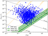 |
Fig. 1. P−Ṗ diagram of the canonical pulsars along with the death line, green solid line, and death valley, shaded green area. |
2.5. Detection
For each pulsar, we checked whether it fulfilled the detection criteria, based on on three factors. First, the beaming fraction indicates the fraction of the sky covered by the radiation beam and depends on the considered wavelength; here that is radio or γ-ray. The beaming fraction varies also with the pulsar spin rate, geometry and location of the emission regions. Before going on to describe how the beaming fraction in radio and γ-ray are computed, it is important to define several angles.
The angle between the line of sight and the rotation axis is denoted by  , where nΩ = Ω/∥Ω∥ is a unit vector along the rotation axis and n the unit vector along the line of sight. The inclination angle
  is the angle between the rotation axis and the magnetic moment, μ being the unit vector along the magnetic moment. Traditionally, the impact angle is also introduced as the angle between the magnetic moment and the line of sight
  . Moreover, it is related to the previous angles by α + β = ξ.
We chose an isotropic distribution for the Earth viewing angle, ξ, as well as for the orientation of the unitary rotation vector. The Cartesian coordinates of the unit rotation vector, nΩ, are (sin θnΩ cos ϕnΩ, sin θnΩ sin ϕnΩ, cos θnΩ). We set the Sun’s position at (x⊙, y⊙, z⊙) = (0 kpc, 8.5 kpc, 15 pc) (Siegert 2019). The coordinates for n are
 (23)
(23)
To compute the pulsar distance from Earth, we use the formula for the distance,
 (24)
(24)
2.5.1. Radio detection model
The beaming fraction in radio depends on the half opening angle of the radio emission cone, ρ, computed according to Lorimer & Kramer (2004) by
 (25)
(25)
where hem is the emission height, P is the spin period of the pulsar, and c is the speed of light. The emission height is taken constant with an average value of hem = 3 × 10⁵ m, estimated from observations of a sample of pulsars by Weltevrede & Johnston (2008), Mitra (2017), Johnston & Karastergiou (2019), Johnston et al. (2023). The cone half-opening angle, ρ, estimated in Eq. (25) holds only for the last open field lines of a magnetic dipole and can only be applied for slow pulsars, where the radio emission altitude is high enough for the multipolar components to decrease significantly and become negligible.
The pulsar is detected in radio if β = |ξ − α|≤ρ or if β = |ξ − (π − α)| ≤ ρ corresponding to the north and south hemisphere, respectively. It must also satisfy the condition α ≥ ρ and α ≤ π − ρ in order to effectively see radio pulsation, because the line of sight must cross the emission cone to observe pulsations. Another useful quantity is the observed width of the radio profile, wr, which is computed as (see Lorimer & Kramer 2004):
 (26)
(26)
The second factor for detection is the luminosity, which is also different between radio and γ-rays. First, concerning the radio flux density, the formula used is the same as in Johnston et al. (2020) for a pulsar at 1.4 GHz, in order to model the detection carried out by the Parkes radio telescope in the southern Galactic plane (Kramer et al. 2003; Lorimer et al. 2006; Cameron et al. 2020) and the Arecibo telescope in the northern plane (Cordes et al. 2006). We note that these two telescopes do not cover all the sky in the southern and northern plane, but we did not implemented any filter in the code. The formula is
 (27)
(27)
where d is the distance in kpc and Fj is the scatter term which is modeled as a Gaussian with a mean of 0.0 and a variance of σ = 0.2. The detection threshold in radio is set by the signal to noise ratio defined by
 (28)
(28)
The pulsar is detected if the signal to noise ratio S/N is greater or equal to 10. Then,  is the minimum flux which is related to the period of rotation P, the width profile of radio emission, wr, and the sensitivity of the survey which is the last factor for detection. This will be detailed later. We directly compute the radio flux, without computing the luminosity in radio that overlooks the fact that the luminosity received will depend on the geometry of the beam.
The third and last factor is the sensitivity, depending on the survey; therefore, on the instrument used and on the pulse profile observed. A pulsar is detected in radio if the signal-to-noise ratio (S/N) is greater than 10, but this ratio depends on the minimum flux, another function of the instrumental sensitivity. With the aim of computing the observed width pulse profile, we use the same formula as Cordes & McLaughlin (2003)
 (29a)
(29a)
 (29b)
(29b)
Equation (29a) takes into account density fluctuations in the interstellar medium (ISM), the dispersion and scattering during the propagation of the radio pulse when interacting with the free electrons. Moreover, the instrumental effect is also taken into account with τsamp, which is the sampling time of the instrument. All this mechanisms lead to a broader pulse profile. In order to determine the influence of the ISM through τDM, the formula of Bates et al. (2014) can be used,
 (30)
(30)
Here, e is the electron charge, me its mass, Δfch the width of frequency of the instrument channel in Hz, f the observing frequency in Hz, and DM the dispersion measure in pc/cm3. Furthermore, in order to determine the influence of scattering by an heterogeneous and turbulent ISM through τscat, the empirical fit relationship from Krishnakumar et al. (2015) is used
 (31)
(31)
Both τDM and τscat are given in units of second (s) and depend on the dispersion measure DM (in units of pc/cm3), which is found for each pulsar by running the code of Yao et al. (2017) converting the distance of a pulsar into the dispersion measure thanks to their state-of-the art model of the Galactic electron density distribution. The radio survey parameters used are the ones from the Parkes Multibeam Pulsar Survey (PMPS) taken from Manchester et al. (2001), see Table 4.
Survey parameters of the Parks Multibeam Pulsar Survey (PMPS).
Concerning Eq. (29b), S0 represents the survey parameters. Johnston et al. (2020) estimated that S0 should approximately be equal to 0.05 mJy to have a signal to noise ratio greater than 10 for normal pulsars in this survey. We chose Eq. (29b) to compute the minimum flux, to decide whether a pulsar will be detected in radio or not; however, it does not reproduce the whole complexity of this quantity which could be computed more precisely (see Eq. (24) of Faucher-Giguère & Kaspi 2006; for instance, where S0 is computed more precisely) even though it remains a good approximation. In addition we only use the parameters of PMPS to compute τDM, we could have also used the parameters of The Pulsar Arecibo L-band Feed Array (PALFA) Survey; however, the differences in the results in the end are not large if we use these parameters. Consequently, it continues to serve as a favorable approximation to exclusively utilise the parameters delineated by PMPS.
2.5.2. γ-ray detection model
The γ-ray emission model relies on the striped wind model, describing γ-ray photons production emanating from the current sheet within the striped wind. To detect the γ-ray, the line of sight of the observer must remain around the equator plane with an inclination angle constrained by |ξ − π/2|≤α. The γ-ray luminosity is extracted from a study of Kalapotharakos et al. (2019), where the authors showed that the luminosity is described by a fundamental plane. The 3D model depends on the magnetic field, B, the spin-down luminosity, Ė, and the cut-off energy, ϵcut. However, in our PPS the cut-off energy is not computed; therefore, we use their 2D version,
 (32)
(32)
The spin-down, Ė, is computed with Eq. (6) and the associated γ-ray flux detected on earth is computed with
 (33)
(33)
where fΩ is a factor depending on the emission model reflecting the anisotropy. For the striped wind model, Pétri (2011) showed that this factor varies between 0.22 and 1.90. Nevertheless, an approximation is made: if α < −ξ + 0.6109, then fΩ = 1.9; otherwise fΩ = 1. As can be observed in Fig. 7 of Pétri (2011), fΩ is usually equal to one of this two values, depending on the value of the inclination angle, α; hence this approximation. The pulsar is detected in gamma depending on the instrumental sensitivity as described below.
The sensitivity in γ-ray is based on the expectation of the Fermi/LAT instrument5. Two conditions are required to count the detection, the first condition is that the source must be bright enough with a sufficiently high flux. If the galactic latitudes of the pulsar is < 2°, then Fmin = 4 × 10⁻¹⁵ W m−2, and if blind searches are assumed, we set Fmin = 16 × 10−15 W m−2. Hence, if the γ-ray flux Fγ is greater than Fmin, the first condition is fulfilled. The second condition concerns the dispersion measure. We set a threshold on the dispersion measure, DM (a similar approach was done in Gonthier et al. 2018 for millisecond γ-ray pulsars), because γ-ray canonical pulsars typically originate from supernova explosions and are associated with regions of recent star formation, such as supernova remnants or star-forming regions. These environments can have higher densities of free electrons, leading to higher DM values for pulsars in these regions, which is why we use this quantity as a discriminator for detection. Therefore, the DM threshold chosen is 15 cm−3 pc, following the lowest value that can be found in the ATNF catalogue for high-energy pulsars. Thus, with these two conditions fulfilled, a pulsar is reported detected in γ-ray.
3. Results
We move to the PPS simulation results. First, we show runs simulating 10 million pulsars with and without a death line, allowing us to generate old pulsars with ages up to 4.1 × 10⁸ yr. Then, we show runs simulating only one million pulsars with ages up to 4.1 × 10⁷ yr, with and without a death line. We explore a possible spin-velocity misalignment effect due to the galactic potential and the impact of the initial spin period distribution, comparing the normal versus log-normal distributions. Finally, the γ-ray simulations and detection are explained in detail.
3.1. Simulating ten millions pulsars
We begin with a sample containing ten million pulsars, showing the impact of the death line. A same study will be done for one million pulsars.
3.1.1. Without a death line
The first set of simulations discarded the death line. The parameters used for these runs are given in Table 5. The total number of pulsars is summarised in Table 6. The quantities Nr, Ng, and Nrg are the number of radio-only, γ-only, and radio-loud γ-ray pulsars, respectively, extracted from our simulation.
Parameters used in the simulations.
Number of pulsars detected without the implementation of the death line.
Compared to the results obtained by Dirson et al. (2022) at very high spin-down luminosity (Ė > 1031 W), the detection rate is almost identical; however, at Ė > 1028 W, substantially fewer pulsars are detected in radio and radio/γ-ray in our work. There are probably two causes for this discrepancy in the number of detected pulsars at high spin-down luminosities, Ė > 1028 W: firstly, the difference in the spin period distribution at birth. Pulsars have a higher probability to start with a higher P0 since the mean of the distribution is higher (in the previous study the mean period was 60 ms while we set it to 129 ms); therefore, the slowing down of the pulsars can only decrease their rotation frequency, Ω. Equation (6) shows that Ė depends on Ω. However, it does not affect the detection rate in γ-rays because usually canonical γ-ray pulsars possess a high Ṗ and a low P (as they are young); therefore, their Ė is higher than for radio pulsars. Secondly, the ISM dispersion and scattering reduces the number of detected radio pulsars, results without the ISM effect are not shown but discarding its impact would lead to much more detected radio pulsars. Nonetheless, in terms of total number of detected radio pulsars, including the Galactic potential increases this number compared to Dirson et al. (2022). This result is expected because of the attractive nature of the potential of the Galaxy. Moreover, in this latter version, the PPS moved pulsars in random spatial directions at constant speed. As a result, many pulsar could not remain bound to the Milky Way in closed orbits which was an artifact that was especially true for old pulsars which could have time to leave the Galaxy.
Figure 2 compares the distribution of simulated and observed spin periods, in red and blue, respectively. However the comparison is not satisfactory because of an excess of pulsars detected in the simulation. Furthermore, this excess is also present in Fig. 3 where the characteristic age of the observed pulsars and the simulated pulsars are plotted. We note that we employ the characteristic ages defined by
 (34)
(34)
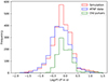 |
Fig. 2. Distribution of the observed period taken from the ATNF catalogue, along with the simulations, without the implementation of the death line. In green, the period of the simulated pulsars with characteristic age greater than 108 yr. |
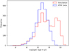 |
Fig. 3. Distribution of the observed age taken from the ATNF catalogue, along with the simulations without the implementation of the death line. |
because we usually do not know the real ages of the observed pulsars.
To verify whether there is a correlation between old pulsars and those with a high spin period, we focus on pulsars with a characteristic age greater than 108 yr, corresponding to the oldest pulsars of the simulation (shown in green in Fig. 2). This coincides with the excess found in Fig. 2. We conclude that canonical pulsars older than 108 yr measured as their real age in our simulations should be discarded at the end of the simulation, since the characteristic age overestimates the real age of pulsars. Indeed, it appears that we are unable to detect canonical pulsars older than 108 yr. The Galactic potential forbids many pulsars to escape from the Milky Way and so, they remain bound to the Galaxy. This is in contrast to the older pulsars found in Dirson et al. (2022) that were escaping the Galaxy easily because of the absence of this potential. Figure 4 shows that many pulsars are in what is commonly called the graveyard of pulsars at the bottom right of the P−Ṗ diagram, the death valley being shown in Fig. 4 but not implemented. Given this excess of long period pulsars when neglecting the death line, we decided to implement it to stick closer to the realistic scenario.
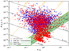 |
Fig. 4. P−Ṗ diagram of the simulated population, along with the observations, without the implementation of the death line. |
3.1.2. With the death line
Adding a death line decreases the number of pulsars detected in radio compared to the situation without a death line, see Table 7. The death line improves the fit as seen in Fig. 5 for the distribution of spin period and compared with Fig. 2, even though there is a slight excess of pulsars which have spin period between 10−0.5 s and 1 s. In Fig. 6, these pulsars in excess lie at Ṗ between 10−18 and 10−17, where there is no data and which correspond to the oldest pulsars in the simulation. Therefore the oldest pulsars simulated here do not correspond to any real data. In addition, too many pulsars end up close to the death line, disagreeing with the observations. The death line creates a pile up effect not seen in the observations.
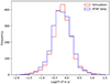 |
Fig. 5. Distribution of the observed period taken from the ATNF catalogue, along with the simulations with the death line implementation. |
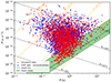 |
Fig. 6. P−Ṗ diagram of the simulated population, along with the observations, with the death line implementation. |
Number of pulsars detected with the death line implementation.
The goodness-of-fit is checked against a density plot of the P−Ṗ diagram as in Johnston & Karastergiou (2017), instead of setting points for individual pulsars. To construct these diagrams, we binned the data evenly in a log scale in P and Ṗ and counted the number of pulsars in each bin. This leads to a 2D histogram to be compared with the observed density plot 2D histogram. Because the total number of simulated pulsars Ntotsim is different from the total number of observed pulsars, Ntotobs, we normalised the number of pulsars in each bin to compare their proportions. We therefore introduce the quantity R as follows
 (35)
(35)
With this definition, the number R remains in the interval [ − 1, +1]. Nsim is the number of pulsar count in a bin of the simulation, Nobs the number of pulsar detected in a bin of the observations. A good fit in a bin corresponds to a value of R close to 0, meaning that the simulation results are close to the observations. Considering Fig. 7, we note a stronger deviation from the observations at the boundaries of the density plot, confirming, for instance, the pile up close to the death line. The high values of R at these boundaries comes from the weak number of pulsars counted in these bins leading to bad statistics and broad variations in the proportions, which are side effects of the density plot approach. The fact that the colors are very dark shows that the proportion of pulsars in most of the bins are not good.
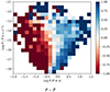 |
Fig. 7. Density plot of the P−Ṗ diagram in comparison with observations. |
A Kolmogorov-Smirnov (KS) test (Smirnov 1948) was conducted on both P and Ṗ, which gave p-values substantially below 0.05 for both quantities, when no death line was implemented. While we obtained p-values of 0.05 for P and well below 0.05 for Ṗ with a death line implementation. The null hypothesis that observations and simulations originate from the same distribution for P cannot be rejected (p-value ≥ 0.05) only when a death line is considered, but is clearly rejected for Ṗ in both case.
3.2. Simulating one million pulsars
3.2.1. With the death line
The parameters used for these runs are shown in Table 5. This new set of simulations is intended to verify if generating pulsars younger than 4.1 × 10⁷ yr is sufficient, since older pulsars are barely observed. The death line is also taken into account. Without any specifications, in all figures (with the exception of Figs. 8, 9, and 10), the simulations were performed while considering the ISM effect.
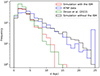 |
Fig. 8. Distance distribution to Earth for observed and simulated populations (one million pulsars), including the death line implementation. |
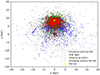 |
Fig. 9. Spatial distribution of the simulated pulsars, along with the observations, projected onto the Galactic plane for one million pulsars simulated. |
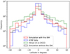 |
Fig. 10. Distribution of the observed latitude taken from the ATNF catalogue, along with the simulations with the death line implementation for one million pulsars simulated. |
Table 8 shows that a few less pulsars were detected in this simulation compared to the one with the death line and ten millions pulsars (see Table 7). Moreover, inspecting the histograms for spin period and spin period derivative respectively in Figs. 11 and 12, we conclude that observations and simulations are very similar in both histograms. A KS test was conducted for both distributions, P and Ṗ, and yielded p-values of 0.67 and 0.17 respectively. Therefore, it is impossible to reject the null hypothesis stating that the simulated distributions are similar to the observed distribution.
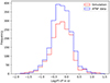 |
Fig. 11. Distribution of the observed period taken from the ATNF catalogue, along with the simulations with the death line implementation for one million pulsars simulated. |
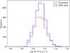 |
Fig. 12. Distribution of the observed period derivative taken from the ATNF catalogue, along with the simulations with the death line implementation for one million pulsars simulated. |
Number of pulsars detected with the death line implementation for one million pulsars simulated.
Fig. 13 shows the good agreement between simulations and observations. Furthermore, comparing Figs. 7 and 14, the former performs better because globally the values of R are close to zero, highlighting the fact that the proportion of pulsars in each 2D bin are almost alike. In addition, the pile up effect close to the death line has been removed from the P−Ṗ diagram, which better fits to the data.
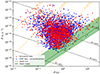 |
Fig. 13. P−Ṗ diagram of the simulated population, along with the observations, with the death line implementation for one million pulsars simulated. |
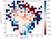 |
Fig. 14. Density plot of the P−Ṗ diagram in comparison with observations for one million pulsars simulated. |
The pulsar distance distribution to Earth is shown in Fig. 8. The improvement compared to Dirson et al. (2022) is marginal. Anyway, we recall here that the estimated distances of the observed pulsars are subject to large uncertainties because of the distances derived from the dispersion measure values (DM) are highly uncertain, while the distances for the simulated pulsars are correct by construction. As a consequence, the comparison between the observed and simulated distance distribution is not a reliable indicator to check the correctness of our model as the discrepancies are subject to observational uncertainties. Fortunately, the P−Ṗ improved compared to the previous work. This could mean the observed pulsars are closer than expected. Indeed, Fig. 9 shows that the positions of the simulated pulsars in the X-Y plane of the Galaxy, including the ISM effect. They are closer to the Sun than the observed pulsars. Surprisingly, by removing the effect of dispersion and scattering of the ISM on the radio pulse profile, we were able to obtain very similar distance distributions between observations and simulations (see Fig. 8). Therefore, a refinement of the ISM impact on radio pulse profiles might help getting a more realistic model.
Finally, Fig. 10 compares the Galactic latitude distributions with the study of Dirson et al. (2022), as displayed in their Fig. 9. In our work, the simulated distribution better matches the observations, especially around all the latitudes away from 0°. Therefore, the Galactic potential helped tracking the pulsar trajectories more realistically. We notice also the ISM removes pulsars close to a latitude of 0°, because the electron density is highest in the galactic plane of the Milky Way.
3.2.2. Without a death line
The simulation with one million simulated pulsars did not allow us to generate pulsars older than 4.1 × 10⁷ yr. We have therefore undertaken a thorough examination of the usefulness of a death line in modeling the canonical pulsar population. Upon conducting simulations with and without a death line (see Table 5 for the parameter values used in the simulations), we found that the resultant number of detected pulsars and the corresponding plots exhibited remarkable similarities. By conducting the KS test on P and Ṗ between two simulations, one with and one without the death line, we obtained p-values of 0.20 and 0.16, respectively. Since both p-values are greater than 0.05, this indicates no significant difference between the two simulations, supporting their similarity. Consequently, our attention turned towards exploring the impact of lower birth rates to ascertain whether they may provide a more congruous fit for both the spin period and spin period derivative distributions.
Running simulations with a birth rate of 1/70 yr−1 or a birth rate of 1/150 yr−1 (thereby increasing the oldest simulated pulsar) conspicuously revealed an insufficient number of detected pulsars (seen in Figs. 15 and 16). Intriguingly, a discernible paucity of pulsars congregating in the bottom right quadrant of the diagram, colloquially known as the pulsar graveyard, persisted even under these conditions. Therefore, regardless of the birth rates, this casts doubt on the necessity of a death line in this configuration. Ultimately, our analysis underscores the pivotal importance of delineating the maximum real age of simulated pulsars, as elucidated in Sect. 3.1, while the incorporation of a death line do not seem indispensable for attaining realistic results when simulating one million pulsars.
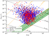 |
Fig. 15. P−Ṗ diagram of the simulated population, along with the observations, without death line implementation and with a birth rate of 1/70 yr−1 for the one million pulsars simulated. |
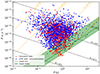 |
Fig. 16. P−Ṗ diagram of the simulated population, along with the observations, without death line implementation, birth rate of 1/150 yr−1 for one million pulsars simulated. |
3.3. Spin-velocity misalignment effect
With the aim of observing the effect of the Galactic potential, we looked at the alignment of the rotation axis and the proper motion velocities of the pulsars. The results are taken from the simulation containing one million pulsars, with the parameters given in Table 5. Noutsos et al. (2013) showed by studying a catalogue of 58 pulsars that pulsars younger than 10 Myr keep their rotation axis and their velocities vector still aligned or anti-aligned, because they were aligned at birth according to Rankin (2007). Meanwhile, pulsars older than 10 Myr do not show this trend anymore. This progressive misalignment effect is due to the movement through the Galactic potential.
Figure 17 demonstrates that most pulsars have their rotation axis aligned or counter-aligned with their velocities, but for spin-velocity angles between 30° and 150° the numbers of pulsars is considerably lower than around alignment 0° and counter-alignment 180°. On the one hand, for pulsars younger than 10 Myr, shown in blue in Fig. 18, only a small fraction of pulsars have their spin-velocity angle greater than 30° and below 150°. On the other hand, for pulsars older than 10 Myr, shown in red in Fig. 18, their spin-velocity angle becomes greater than 30° or smaller than 150°.
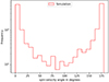 |
Fig. 17. Distribution of the spin-velocity angles for all the detected pulsars in the simulation for the one million pulsars simulated. |
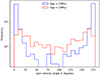 |
Fig. 18. Distribution of the spin-velocity angles for the detected pulsars younger than 10 Myr (blue) and pulsars older than 10 Myr (red) in the simulation. |
Furthermore, Fig. 19 confirms that, the older the pulsar is, the better its chance to perform several orbits in the Galaxy, allowing it to significantly deviate from spin-velocity alignment or anti-alignment. In addition, even for pulsars that are not as old, their spin-velocity angle will evolve between 30° and 150° to give them the ability to perform many orbits in the Galaxy. This supports the idea that the Galactic potential is responsible for the misalignment irrespective of the age of the pulsar. The opposite is also true, some old pulsars do not perform many orbits (but most of them are) and, as a consequence, they (approximately) retain their spin-velocity alignment or misalignment. The previous plots clearly highlight the influence of the Galactic potential making pulsars lose their alignment between their rotation axis and their proper motion velocities through time.
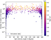 |
Fig. 19. Spin-velocity angles for the detected pulsars in function of the number of orbits made by the pulsars in this study. |
3.4. Log normal vs normal distribution for spin period at birth
To estimate the impact of the spin period distribution at birth, we compare the results of the log-normal law with the previously used normal law in Dirson et al. (2022):
 (36)
(36)
The simulation in this subsection uses the parameters listed in the two first columns of Table 9 and to be put into Eq. (36). The Galactic potential and the death line were both taken into account to compare the influence of the initial spin period distribution on the one million pulsars simulated, see Table 5 for the parameters used. In Table 9, only the results for σp = 30 ms are shown because other values have been tried out, namely 10 ms, 20 ms and 40 ms, but gave no higher p-values than for σp = 30 ms. Moreover, we chose  from 60 ms to 140 ms because it is the range usually used in other work (Faucher-Giguère & Kaspi 2006; Gullón et al. 2014; Dirson et al. 2022).
P-values and total number of pulsars detected (Ndetection) obtained for simulations with different  for the Gaussian initial distribution of spin period.
Table 9 highlights the fact that for  above 60 ms and below 140 ms, an acceptable p-value ≥ 0.05 is reached for the Ṗ distribution. However no matter the value of
  , a satisfying p-value for the P distribution is not reached in contrary to the log-normal distribution at birth, for which satisfying p-value for both distributions were obtained. We conclude that the initial distribution for the spin period found by Igoshev et al. (2022) allows us to better reproduce the canonical pulsar population.
3.5. γ-ray detection
We go on to focus on the γ-ray pulsar population. First, we note that the total number of pulsars detected is significantly larger in our sample (307 detections) compared to the observations (173 detections), when using the Fermi/LAT instrument sensitivity. However, the simulated γ-ray only and radio loud γ-ray pulsars are in the expected area of Fig. 20, furthermore, the KS test gives a p-value of 0.52 and ≈0 for Ṗ and P, respectively. The null hypothesis can not be rejected for Ṗ but it is rejected for P. However, when the KS test is conducted on the γ-ray population only we get p-values of 0.03 and 0.14 for Ṗ and P, respectively; therefore, here the null hypothesis is rejected for Ṗ but not for P. While for the radio loud γ-ray population p-values of 0.11 and ≈0 are obtained for Ṗ and P, respectively. Thus, we thought the low p-value obtained for P for both population was probably because of the seven high-spin period radio loud γ-ray pulsars (seen in Fig. 20). However, even conducting the KS test without these pulsars gives a p-value ≥ 0.05 for Ṗ and well below 0.05 for P.
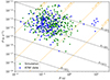 |
Fig. 20. P−Ṗ diagram of the γ-only pulsars for both the simulations and the observations, with one million pulsars simulated. |
In addition, we also compared the γ-ray flux distribution of the simulated and observed populations. In Fig. 21, we notice that both distributions peak at the same flux level around 10−13.7 W m−2. Globally, the number of pulsars in the simulation with a flux greater than 10−13.4 W m−2 is very close to the observations. However, between 10−14.4 W m−2 and 10−14 W m−2, there are much more pulsars in the simulation. This bi-modality in the simulated γ -ray flux distribution is an artefact introduced by our abrupt condition on the threshold, Fmin, depending on the radio detection of a pulsar and on a sufficiently low galactic latitude. However if we smoothly change Fmin from 4 × 10⁻¹⁵ to 16 × 10−15 (the two Fmin values used in this work), the bi-modality would almost disappear.
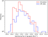 |
Fig. 21. Distribution of the γ-ray flux of the simulated population along with the observations from the 3PC catalogue. |
Finally, we can compare the simulated and observed γ-ray light-curve peak separation Δ in Fig. 22. The separation Δ is computed according to Pétri (2011) by
 (37)
(37)
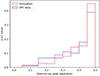 |
Fig. 22. Distribution of the γ-ray peak separation of the simulated population along with the observations from the 3PC catalogue. |
where ξ is the angle between the line of sight and the rotation axis and α the inclination angle. The distributions are normalised in order to obtain probability distribution functions (pdf) for both observations and simulations. The normalisation is performed by dividing each distribution function by its total number of pulsars, whether observed or simulated. Moreover, Δ is constrained to the interval between 0 and 0.5, because we consider that peak separations, Δ, larger than 0.5 can be scaled to Δ = 1 − Δ by a phase shift, since the signal is periodic and represents the phase separation between two peaks and the definition of the first or main peak is arbitrary. Figure 22 displays a remarkable similarity between the observed and simulated distributions of the γ-ray peak separation, meaning the striped wind model captures this geometric feature very well.
The higher number of detected pulsars in the simulations could be related to the unidentified sources in the Fourth Fermi-LAT catalogue of γ-ray sources (4FGL). Since many unidentified Galactic sources are listed in this catalogue, many γ-ray pulsars might have been observed without being identified as such yet. Nonetheless, assuming that every unidentified γ-ray pulsar in this catalogue will be recognised as such by a future more sensitive instrument and that a significant difference between the number of simulated and observed pulsars subsists, this could hint to some shortcomings faced by the striped wind model. We note that some of these possible flaws of geometrical or physical nature. First the γ-ray beam opening angle could be smaller than the one used due to some plasma recollimation effect within the striped wind. This would reduce the number of detected pulsars. Secondly, the luminosity function could also deviate from the prescription adopted in Eq. (32). Another dependence on B and P or equivalently on P and Ṗ could be introduced, maybe adding a third parameter like the cut-off energy to better describe the γ-ray luminosity. Furthermore, we compare our results with the PPS work of Pierbattista et al. (2012), where they simulated the young γ-ray pulsar population with four different models: outer gap (OG), slot gap (SG), polar cap (PC), and outer polar cap (OPC) models. To summarise their findings, their best model is the OPC model, showing almost identical results as ours, P−Ṗ shape and number of detections, except that we detect γ-ray pulsars a little farther away from Earth.
To conclude the part about γ-ray pulsars, we predict the number of pulsars that would be detected by a future instrument, ten times more sensitive than Fermi/LAT. We asked the question: what if we run another simulation with the same parameters as in Table 5, only changing the threshold of detection for γ-ray? This investigation could help in identifying the nature of the GeV excess in the Galactic centre. Therefore, we decreased the instrument sensitivity Fmin by a factor 10: if the galactic latitudes of the pulsar is < 2°, then Fmin = 0.4 × 10⁻¹⁵ W m−2; concerning blind searches, we set Fmin = 1.6 × 10⁻¹⁵ W m−2.
The γ-ray detected pulsar positions in the X-Y plane of the Galaxy are shown in Fig. 23. In this simulation, 2492 γ-ray pulsars are detected, in green, being γ-ray only or radio-loud γ-ray pulsars, among them only 350 (really close to the number of γ-ray and radio/γ-ray pulsars detected in Sect. 3.2) would have been detected if the same sensitivity as before was kept, in red in Fig. 23. Therefore we detected seven times more γ-ray pulsars compared to the number found with the previous sensitivity. Furthermore, the other 2142 pulsars, in green in Fig. 23, detected with this increased sensitivity highlight several interesting features. We obviously detect more pulsars close to Earth, and also many more in the centre of the Galaxy. This result indicates that the GeV excess in the Galactic centre could be linked to pulsars not yet identified, while usually the origin of this GeV excess is attributed to self-annihilating dark matter particles (Hooper 2022). However, millisecond pulsars, not modeled in this work, could also contribute significantly to this GeV excess.
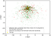 |
Fig. 23. Spatial distribution of the simulated γ-ray detected pulsars, projected onto the Galactic plane for one million pulsars simulated, with a lower Fmin. |
4. Discussion
For the initial spin period distribution, Igoshev et al. (2022) suggested values for the mean period Pmean in the range from approximately 57 ms to 129 ms and for its spread, σp, the range from 0.45 to 0.65. The values Pmean = 129 ms and σp = 0.45 are best educated guesses. However, further investigations on this work could benefit from an automated method to find the best set of values. Hence, we are currently working on an optimisation algorithm to find the optimal initial parameters for the population synthesis, not only for the spin period, but for the whole parameter space presented in Table 5. Our optimisation algorithm will help to constrain the properties of the Milky Way pulsar population by constraining parameters such as the birth rate, which is supposed to be between 1/33 yr−1 and 1/150 yr−1. More details are given in Faucher-Giguère & Kaspi (2006), Gullón et al. (2014) or Johnston & Karastergiou (2017).
In the main part of the paper, we abstain from showing outcomes stemming from simulations featuring a constant magnetic field. However, we ran simulations that clearly highlight the inferior performance of a simulation without magnetic field evolution (see Appendix B). Moreover, Appendix C explores different parameter spaces for the PPS, allowing us to meticulously scrutinise whether the parameters showcased in the main part of the paper optimally reflect the observational data. This work demonstrates that even if a substantial number of parameters are required for the PPS, they can be meaningfully constrained by such studies with reasonable accuracy.
Furthermore, in Sect. 3.5, we explored the results when the sensitivity in γ-ray is increased by a factor of 10. We have not discussed any improvements in the radio detection yet, while we run a simulation by increasing the sensitivity by a factor of 50 to match approximately the properties of SKA (McMullin et al. 2020). The result of this simulation with an increased sensitivity led to 52276 pulsars detected (when simulating one million pulsars, with a death line), which is approximately 31 times more than with the sensitivity of Parkes and Arecibo telescopes.
We emphasise that the death valley strongly depends on the chosen model. For instance the radio luminosity law plays a central role, we assumed that  with α = 1/4 (see Eq. (27)) according to Johnston & Karastergiou (2017) and Johnston et al. (2020), where they found it to be the best fit to the data. Following their conclusion we decided not to choose α as another parameter. However it would impact the death valley, but this effect is not considered in our work. Furthermore, in other works such as Graber et al. (2024) for instance, they do not explicitly use a death valley because they use a different radio luminosity law, meaning a different value for α and adjust the magnetic field decay time accordingly. We stress that this is just another method to deal with the bottom right corner of the P−Ṗ diagram, where pulsars are likely to stop emitting photons, since the death valley removes pulsars based on a combination of P and Ṗ. Graber et al. (2024) PPS is based on a phenomenological approach where the radio luminosity is tuned to conform to observations. In our approach, adding a death valley is based on more physical grounds, which are related to the micro-physics close to the neutron star polar cap.
5. Summary
Without the implementation of the Galactic potential, in the PPS of Dirson et al. (2022), the pulsars were moving in straight lines along one direction chosen randomly for each pulsar. This evolution of the proper motion was not realistic, even though the evolution model had already replicated a significant portion of the canonical pulsar population. However all the new improvements put into this PPS, meaning the Galactic potential, the effect of the ISM on the radio pulse profiles and the fact that the decay timescale of the magnetic field is taken randomly within a certain range, allow for a more accurate reproduction of the population in the P−Ṗ diagram.
The first results where we emulate ten millions pulsars showed an excess of old pulsars detected in the simulation. In the P−Ṗ diagram we saw that this excess was associated to pulsars that lie below the death line, and are, thus, no longer creating any more pairs. With this finding, we realised that it was imperative to implement the death line. The results obtained with the death line were then in better agreement with observations when plotting the most relevant distributions, such as period and period derivative.
Nonetheless, simulating one million pulsars had allowed us to demonstrate that with or without a death line the results were alike and therefore, in the case where the oldest simulated pulsar is 4.1 × 10⁷ yr (its real age), a death line is not necessary to explain the observations. In this paper we showed two approaches to reproduce the observed canonical pulsar population; however, when we consider the approach where the oldest pulsar simulated is only 4.1 × 10⁷ yr, we state that no older pulsars might be detected with our current telescopes in the Galaxy. Meanwhile, the Milky Way is very much older than this and has thus been forming pulsars since its beginning. There is apparently no reason not to simulate pulsars that are older than 108 yr. If there is one, we do not know it, as they become harder to detect because of their wide pulse profile with their age, but some could still be detectable. If this is the case, then it means that the death line is not necessary in pulsar population synthesis to explain observations. When the simulation is ran with ten millions pulsars, the death line becomes a necessity. However this simulation gives results less similar to observations.
It has also been shown that old pulsars with age larger than 10 Myr have a tendency to lose their alignment between rotation axis and velocity, a direct effect of the Galactic potential as shown by the observations of Noutsos et al. (2013). This is the first time it has been done in a simulation.
The striped wind model seems to reproduce the γ-ray population of canonical pulsars well according to the p-value of the KS test greater than 0.05 for Ṗ. However the KS test gives a p-value lower than 0.05 for P; yet there are several observed radio-loud γ-ray pulsars that the simulation struggles to reproduce (not only the ones with high P) but which might explain this low p-value. However in the simulation a higher number of these pulsars are detected compared to observations. This probably indicates that a part of the unidentified sources from the 4FGL catalogue are pulsars. Testing an instruments with improved sensitivity for the detection of γ-ray pulsars lead us to the conclusion that part of the GeV excess in the Galactic centre could be young γ-ray pulsars. Moreover, the assumption that millisecond pulsars could also contribute to this excess will be checked once a PPS model for millisecond pulsars will be available. The most common picture suppose that only millisecond pulsars are responsible for this excess, while we demonstrated that young γ-ray pulsars could also play a significant role.
In summary, the best parameters found for this pulsar population synthesis are for Pmean = 129 ms, σp = 0.45 for the log-normal spin period distribution at birth, Bmean = 2.75 × 10⁸ T, σb = 0.5 for the magnetic field distribution at birth and for a birth rate of 1/41 yr−1. Ultimately, this work provides a simulated population of pulsars within the Milky Way that is more similar to the observations, compared to Johnston et al. (2020) and Dirson et al. (2022), the two most recent population synthesis considering both radio and γ-ray emission. Moreover, such investigations are useful for predicting the detection rate of future radio surveys, such as SKA or New Extension in Nançay Upgrading the Low Frequency Array (NenuFAR).
The PPS method developed in this paper can be extended to other pulsar populations in the Milky Way, such as millisecond pulsars and magnetars. Magnetars, for instance, would need another distribution scenario at birth for their magnetic field that takes into account the emission in X-rays and with a faster decay for the magnetic field. The magnetars are located just above the canonical pulsars in the P−Ṗ diagram, at the top-right of the diagram. A more complex population is the recycled (or millisecond pulsars) ‘brought back to life’ by accreting matter from a companion star. This accretion mechanism spins up the neutron stars moving them from the graveyard of pulsars to the bottom left of the P−Ṗ diagram, crossing again the death line in the opposite sense and allowing them to be revived by creating electron-positron pair cascades again. However, they are difficult to model because their evolution scenario must take into account their accretion phase and spin-up. We are currently working on both these populations to reproduce them in a PPS that is based on the methods and findings in this work.
Acknowledgments
This work has been supported by the grant ANR-20-CE31-0010. We acknowledge the High Performance Computing Centre of the University of Strasbourg for supporting this work by providing scientific support and access to computing resources. D.M. acknowledges the support of the Department of Atomic Energy, Government of India, under project No. 12-R&DTFR-5.02-0700 and grant 2020/37/B/ST9/02215 from the National Science Centre, Poland.
References
- Abdo, A. A., Ajello, M., Allafort, A., et al. 2013, ApJS, 208, 17 [Google Scholar]
- Arons, J. 1983, ApJ, 266, 215 [CrossRef] [Google Scholar]
- Bajkova, A. T., & Bobylev, V. V. 2021, Astron. Astrophys. Trans., 32, 177 [NASA ADS] [CrossRef] [Google Scholar]
- Bates, S. D., Lorimer, D. R., Rane, A., & Swiggum, J. 2014, MNRAS, 439, 2893 [NASA ADS] [CrossRef] [Google Scholar]
- Bogdanov, S., Lamb, F. K., Mahmoodifar, S., et al. 2019, ApJ, 887, L26 [NASA ADS] [CrossRef] [Google Scholar]
- Bovy, J. 2015, ApJS, 216, 29 [NASA ADS] [CrossRef] [Google Scholar]
- Cameron, A. D., Champion, D. J., Bailes, M., et al. 2020, MNRAS, 493, 1063 [NASA ADS] [CrossRef] [Google Scholar]
- Chen, K., & Ruderman, M. 1993, ApJ, 402, 264 [NASA ADS] [CrossRef] [Google Scholar]
- Cheng, K. S., Ho, C., & Ruderman, M. 1986, ApJ, 300, 500 [CrossRef] [Google Scholar]
- Cordes, J. M., & McLaughlin, M. A. 2003, ApJ, 596, 1142 [NASA ADS] [CrossRef] [Google Scholar]
- Cordes, J. M., Freire, P. C. C., Lorimer, D. R., et al. 2006, ApJ, 637, 446 [NASA ADS] [CrossRef] [Google Scholar]
- Daugherty, J. K., & Harding, A. K. 1982, ApJ, 252, 337 [NASA ADS] [CrossRef] [Google Scholar]
- Daugherty, J. K., & Harding, A. K. 1996, ApJ, 458, 278 [NASA ADS] [CrossRef] [Google Scholar]
- Dirson, L., Pétri, J., & Mitra, D. 2022, A&A, 667, A82 [NASA ADS] [CrossRef] [EDP Sciences] [Google Scholar]
- Faucher-Giguère, C.-A., & Kaspi, V. M. 2006, ApJ, 643, 332 [CrossRef] [Google Scholar]
- Forest, E., & Ruth, R. D. 1990, Phys. D Nonlinear Phenom., 43, 109 [Google Scholar]
- Gil, J., & Mitra, D. 2001, ApJ, 550, 383 [NASA ADS] [CrossRef] [Google Scholar]
- Gonthier, P. L., Ouellette, M. S., Berrier, J., et al. 2002, ApJ, 565, 482 [NASA ADS] [CrossRef] [Google Scholar]
- Gonthier, P. L., Harding, A. K., Ferrara, E. C., et al. 2018, ApJ, 863, 199 [NASA ADS] [CrossRef] [Google Scholar]
- Graber, V., Ronchi, M., Pardo-Araujo, C., et al. 2024, ApJ, 968, 16 [CrossRef] [Google Scholar]
- Gullón, M., Miralles, J. A., Viganò, D., & Pons, J. A. 2014, MNRAS, 443, 1891 [CrossRef] [Google Scholar]
- Harding, A. K., & Muslimov, A. G. 2011, ApJ, 743, 181 [NASA ADS] [CrossRef] [Google Scholar]
- Harding, A. K., Stern, J. V., Dyks, J., & Frackowiak, M. 2008, ApJ, 680, 1378 [NASA ADS] [CrossRef] [Google Scholar]
- Hewish, A., Bell, S. J., Pilkington, J. D. H., et al. 1969, Nature, 224, 472 [NASA ADS] [CrossRef] [Google Scholar]
- Hirotani, K. 2008, ApJ, 688, L25 [NASA ADS] [CrossRef] [Google Scholar]
- Hobbs, G., Lorimer, D. R., Lyne, A. G., & Kramer, M. 2005, MNRAS, 360, 974 [Google Scholar]
- Hofmann, W., & Zanin, R. 2023, ArXiv e-prints [arXiv:2305.12888] [Google Scholar]
- Hooper, D. 2022, ArXiv e-prints [arXiv:2209.14370] [Google Scholar]
- Igoshev, A. P., Frantsuzova, A., Gourgouliatos, K. N., et al. 2022, MNRAS, 514, 4606 [CrossRef] [Google Scholar]
- Jawor, J. A., & Tauris, T. M. 2022, MNRAS, 509, 634 [Google Scholar]
- Johnston, S., & Karastergiou, A. 2017, MNRAS, 467, 3493 [CrossRef] [Google Scholar]
- Johnston, S., & Karastergiou, A. 2019, MNRAS, 485, 640 [NASA ADS] [CrossRef] [Google Scholar]
- Johnston, S., Smith, D. A., Karastergiou, A., et al. 2020, MNRAS, 497, 1957 [NASA ADS] [CrossRef] [Google Scholar]
- Johnston, S., Kramer, M., Karastergiou, A., et al. 2023, MNRAS, 520, 4801 [Google Scholar]
- Kalapotharakos, C., Harding, A. K., Kazanas, D., & Wadiasingh, Z. 2019, ApJ, 883, L4 [NASA ADS] [CrossRef] [Google Scholar]
- Kramer, M., Bell, J. F., Manchester, R. N., et al. 2003, MNRAS, 342, 1299 [NASA ADS] [CrossRef] [Google Scholar]
- Krishnakumar, M. A., Mitra, D., Naidu, A., Joshi, B. C., & Manoharan, P. K. 2015, ApJ, 804, 23 [NASA ADS] [CrossRef] [Google Scholar]
- Li, C., Zhao, G., Jia, Y., et al. 2019, ApJ, 871, 208 [Google Scholar]
- Lorimer, D. R., & Kramer, M. 2004, Handbook of Pulsar Astronomy (Cambridge: Cambridge University Press) [Google Scholar]
- Lorimer, D. R., Stairs, I. H., Freire, P. C., et al. 2006, ApJ, 640, 428 [NASA ADS] [CrossRef] [Google Scholar]
- Manchester, R. N., Lyne, A. G., Camilo, F., et al. 2001, MNRAS, 328, 17 [NASA ADS] [CrossRef] [Google Scholar]
- Manchester, R. N., Hobbs, G. B., Teoh, A., & Hobbs, M. 2005, AJ, 129, 1993 [Google Scholar]
- McMullin, J., Diamond, P., McPherson, A., et al. 2020, Proc. SPIE, 11445, 1144512 [NASA ADS] [Google Scholar]
- Mitra, D. 2017, JApA, 38, 52 [NASA ADS] [Google Scholar]
- Mitra, D., Basu, R., Melikidze, G. I., et al. 2020, MNRAS, 492, 2468 [NASA ADS] [CrossRef] [Google Scholar]
- Miyamoto, M., & Nagai, R. 1975, PASJ, 27, 533 [NASA ADS] [Google Scholar]
- Muslimov, A. G., & Harding, A. K. 2004, ApJ, 617, 471 [NASA ADS] [CrossRef] [Google Scholar]
- Navarro, J. F., Frenk, C. S., & White, S. D. M. 1997, ApJ, 490, 493 [Google Scholar]
- Noutsos, A., Schnitzeler, D. H. F. M., Keane, E. F., et al. 2013, MNRAS, 430, 2281 [NASA ADS] [CrossRef] [Google Scholar]
- Paczynski, B. 1990, ApJ, 348, 485 [NASA ADS] [CrossRef] [Google Scholar]
- Pétri, J. 2009, A&A, 503, 13 [NASA ADS] [CrossRef] [EDP Sciences] [Google Scholar]
- Pétri, J. 2011, MNRAS, 412, 1870 [Google Scholar]
- Pétri, J. 2012, MNRAS, 424, 605 [Google Scholar]
- Philippov, A., Tchekhovskoy, A., & Li, J. G. 2014, MNRAS, 441, 1879 [NASA ADS] [CrossRef] [Google Scholar]
- Pierbattista, M., Grenier, I. A., Harding, A. K., et al. 2012, A&A, 545, A42 [NASA ADS] [CrossRef] [EDP Sciences] [Google Scholar]
- Popov, S. B., Pons, J. A., Miralles, J. A., et al. 2010, MNRAS, 401, 2675 [NASA ADS] [CrossRef] [Google Scholar]
- Rankin, J. M. 2007, ApJ, 664, 443 [CrossRef] [Google Scholar]
- Riley, T. E., Watts, A. L., Bogdanov, S., et al. 2019, ApJ, 887, L21 [Google Scholar]
- Ronchi, M., Graber, V., Garcia-Garcia, A., et al. 2021, ApJ, 916, 100 [NASA ADS] [CrossRef] [Google Scholar]
- Ruderman, M. A., & Sutherland, P. G. 1975, ApJ, 196, 51 [Google Scholar]
- Siegert, T. 2019, A&A, 632, L1 [NASA ADS] [CrossRef] [EDP Sciences] [Google Scholar]
- Skowron, D. M., Skowron, J., Mróz, P., et al. 2019, Science, 365, 478 [Google Scholar]
- Smirnov, N. 1948, Ann. Math. Stat., 19, 279 [CrossRef] [Google Scholar]
- Smith, D. A., Bruel, P., Cognard, I., et al. 2019, ApJ, 871, 78 [NASA ADS] [CrossRef] [Google Scholar]
- Smith, D. A., Abdollahi, S., Ajello, M., et al. 2023, ApJ, 958, 191 [NASA ADS] [CrossRef] [Google Scholar]
- Spitkovsky, A. 2006, ApJ, 648, L51 [Google Scholar]
- Sturrock, P. A. 1971, ApJ, 164, 529 [Google Scholar]
- Takata, J., Wang, Y., & Cheng, K. S. 2011, ApJ, 726, 44 [Google Scholar]
- Viganò, D. 2013, ArXiv e-prints [arXiv:1310.1243] [Google Scholar]
- Viganò, D., Rea, N., Pons, J. A., et al. 2013, MNRAS, 434, 123 [CrossRef] [Google Scholar]
- Watters, K. P., & Romani, R. W. 2011, ApJ, 727, 123 [NASA ADS] [CrossRef] [Google Scholar]
- Weltevrede, P., & Johnston, S. 2008, MNRAS, 391, 1210 [NASA ADS] [CrossRef] [Google Scholar]
- Yadigaroglu, I.-A., & Romani, R. W. 1995, ApJ, 449, 211 [NASA ADS] [CrossRef] [Google Scholar]
- Yao, J. M., Manchester, R. N., & Wang, N. 2017, ApJ, 835, 29 [NASA ADS] [CrossRef] [Google Scholar]
- Yusifov, I., & Küçük, I. 2004, A&A, 422, 545 [NASA ADS] [CrossRef] [EDP Sciences] [Google Scholar]
- Zhang, B., Harding, A. K., & Muslimov, A. G. 2000, ApJ, 531, L135 [NASA ADS] [CrossRef] [Google Scholar]
Appendix A: The integration scheme used
A.1. The scheme
One of the new aspect in this work is to solve the equation of motion, Eq. (13), namely, to follow more realistically the motion of our sample of pulsars. To achieve this objective we implemented a fourth-order integration scheme called Position Extended Forest Ruth-Like (PEFRL). This algorithm was chosen because of its high order, allowing for a high precision on the trajectory of the pulsar. In addition, it is a symplectic algorithm, meaning that it conserves the total energy of the pulsar (kinetic plus potential), minimising the error even if the integration is done for a long time with any orbits. It works in the same way as a Verlet scheme of second order, the velocities and coordinates are shifted separately, but in the end they get synchronised. The different steps of the algorithm are as follows.
 (A.1a)
 (A.1b)
 (A.1c)
 (A.1d)
 (A.1e)
 (A.1f)
 (A.1g)
 (A.1h)
 (A.1i)
Here, r is the position vector, v is the velocity vector, h is the time step, ∇Φ is the gradient of the potential and n is the time at which we compute the position or the velocity. λ, ξ and χ are constants that are tabulated in Table A.1; see for instance Forest & Ruth (1990).
Value of the constants used for the PEFRL scheme.
A.2. Precision of the PEFRL algorithm
Before implementing the gravitational potential and the integration scheme in the whole synthesis, the precision of the trajectory of a single pulsar in the Milky Way was checked. The initial conditions for the pulsar are the following: x = 5.1 kpc, y = −1.9 kpc, z = 0.05 kpc, vx = −47.8 km/s vy = 97.0 km/s, and vz = 22.6 km/s. Those initial conditions were chosen randomly, the only constrain being to have the pulsar in the Galaxy with realistic coordinates on the one hand and with realistic speeds for a pulsar on the other hand. Furthermore, the total integration time is 1.25 Gyr and the time step used is 105 yr. In order to check the precision of the scheme, the total energy of the pulsar, sum of the kinetic plus potential energy, that should be conserved is computed as
 (A.2)
(A.2)
The trajectory obtained after the integration with the PEFRL algorithm is shown in Fig. A.1. This trajectory shows that the pulsar, with these initial conditions, remains bound to the Galaxy. The pulsar here takes approximately 201.3 Myr to complete an orbit in the Galaxy. The time step chosen is significantly smaller than the orbital period (h/Porb = 0.0005), and we obtain approximately 6 orbits by integrating the trajectory during 1.25 Gyr. Bajkova & Bobylev (2021) showed several trajectories in their paper, the one obtained here seems coherent compared to the different trajectories that they got.
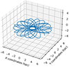 |
Fig. A.1. Trajectory of a single pulsar in the Galactocentric frame. |
Figure A.2 shows the relative error on the total energy. It is indeed almost constant along the whole integration of the trajectory. The maximum relative error on the energy is of the order of 10−9, a very good accuracy for this trajectory. Globally, when a single pulsar has its trajectory integrated in the PPS, the relative error is at maximum 0.001 and the minimum seen was 10−14.
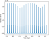 |
Fig. A.2. Relative error on the energy of a single pulsar in the Galactocentric frame. |
Appendix B: Results for a constant magnetic field
Depending on the PPS, the magnetic field will be considered constant (Johnston & Karastergiou 2017; Faucher-Giguère & Kaspi 2006) or decaying (Gullón et al. 2014; Dirson et al. 2022; Jawor & Tauris 2022). The goal is here is to show the results with a constant magnetic field in order to see which model is better between the decaying magnetic field and the constant magnetic field.
Hence, this simulation was run with 30 million pulsar simulated (meaning the oldest pulsar simulated is 1.23 × 10⁹ yr), with a death line and without a decaying magnetic field. The KS test gave p-values of 1.03 × 10⁻²² and 3.38 × 10−51 for P and Ṗ, respectively; therefore the null hypothesis is rejected for both P and Ṗ. Here we simulate more pulsars than in the main part of the paper, since if we simulate with the same number of pulsars, it seems the whole P−Ṗ diagram is not covered. Therefore if a constant magnetic field was the best way to reproduce the canonical population, it means we would detect much older pulsars than with the magnetic field decay prescription. The parameters used are in Table 5. It gives results less close to the observations than with a decaying magnetic field. As can be seen in Fig. B.1, too many pulsars from the simulation appear on the top right of the diagram and almost none at the bottom. In Table B.1, we note a total of pulsars which is smaller from what we found for all of our previous results in Sect. 3. We could expect to reproduce equally well the population of observed pulsars with a constant magnetic field, however compared to the study of Johnston & Karastergiou (2017) where they used this assumption for the magnetic field, we do not evolve the braking index. In our simulations, we have  ,
,  and
and  whereas in their simulation
  ,
,  and
and  . Having either the braking index or the magnetic field evolve, allows us to reproduce well the population of pulsars.
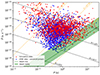 |
Fig. B.1. P−Ṗ diagram of the simulated population, along with the observations, with the death line implementation and a constant magnetic field for each pulsar. |
Number of pulsars detected for the simulation with constant magnetic field for each pulsar and the death line implementation.
Appendix C: Influence of the different parameters
This appendix shows that the parameters chosen in the main part of this paper are meticulously picked and that the uncertainties brought by the large number of parameters is manageable. Multiple simulations were conducted by varying parameter values for the initial distributions, demonstrating that deviations from the optimal values lead to poor results. The simulations were run with in the same conditions as Sect. 3.2, with only one parameter changing between the different sets of simulations and without implementing the ISM, because it would be too time consuming to perform all these simulations. As a consequence in the tables from C.1 to C.5), the p-values are low, while when including the ISM effect they become larger. Therefore, the results and conclusions presented in this section are based on this simplification, which was primarily used to guide the choice of parameters. While these assumptions have helped to identify efficient parameters, it is important to stress that the proposed values are not necessarily optimal. They serve primarily as a foundation for refining the parameters under more realistic conditions. That is why before validating a parameter we checked that the p-values were satisfactory when including the ISM. We found each time a higher p-values.
D-value for different Pmean.
D-value for different Bmean.
D-value for different σb.
D-value for different σp.
D-value for different birth rate (BR).
In order to get an idea on a good range of values for the parameters, the d-values and p-values obtained thanks to the KS test are shown in Table C.1, C.2, C.3, C.4, and C.5. For each parameter, ten simulations were performed in order to get a mean and a standard deviation for the d-values and p-values associated. These simulations helped finding the best values for the parameters by considering the parameter is well constrained when its d-values for both distribution of P and Ṗ are below or close to 0.05 (meaning 5% similarity between the observed and simulated distributions), especially if the previous and next parameter values have higher d-values and lower p-values. As usual p-values above 0.05 means that the null hypothesis can not be rejected, however as explained above, without the ISM effect taken into account the p-values for the Ṗ distribution do not get too high here. Even though it is not an optimisation (and therefore the results can be improved on that point), it allows us to conclude that Pmean must be between 120 ms and 135 ms, with 129 ms as best value. Bmean must be between 2.25 × 10⁸ T and 2.8 × 10⁸ T, with 2.75 × 10⁸ T as best value. σb is well constrained between 0.49 and 0.51, with 0.5 as best value. While σp must be between 0.42 and 0.47, with 0.45 as best value. Finally, the birth rate must be between 1/37 yr−1 and 1/45 yr−1, with 1/41 yr−1 as best value.
All Tables
Number of known canonical pulsars, with spin-down luminosity, Ė, above and below 1028 W, and above 1031 W.
Number of pulsars detected with the death line implementation for one million pulsars simulated.
P-values and total number of pulsars detected (Ndetection) obtained for simulations with different for the Gaussian initial distribution of spin period.
Number of pulsars detected for the simulation with constant magnetic field for each pulsar and the death line implementation.
All Figures
|
Fig. 1. P−Ṗ diagram of the canonical pulsars along with the death line, green solid line, and death valley, shaded green area. |
| In the text | |
|
Fig. 2. Distribution of the observed period taken from the ATNF catalogue, along with the simulations, without the implementation of the death line. In green, the period of the simulated pulsars with characteristic age greater than 108 yr. |
| In the text | |
|
Fig. 3. Distribution of the observed age taken from the ATNF catalogue, along with the simulations without the implementation of the death line. |
| In the text | |
|
Fig. 4. P−Ṗ diagram of the simulated population, along with the observations, without the implementation of the death line. |
| In the text | |
|
Fig. 5. Distribution of the observed period taken from the ATNF catalogue, along with the simulations with the death line implementation. |
| In the text | |
|
Fig. 6. P−Ṗ diagram of the simulated population, along with the observations, with the death line implementation. |
| In the text | |
|
Fig. 7. Density plot of the P−Ṗ diagram in comparison with observations. |
| In the text | |
|
Fig. 8. Distance distribution to Earth for observed and simulated populations (one million pulsars), including the death line implementation. |
| In the text | |
|
Fig. 9. Spatial distribution of the simulated pulsars, along with the observations, projected onto the Galactic plane for one million pulsars simulated. |
| In the text | |
|
Fig. 10. Distribution of the observed latitude taken from the ATNF catalogue, along with the simulations with the death line implementation for one million pulsars simulated. |
| In the text | |
|
Fig. 11. Distribution of the observed period taken from the ATNF catalogue, along with the simulations with the death line implementation for one million pulsars simulated. |
| In the text | |
|
Fig. 12. Distribution of the observed period derivative taken from the ATNF catalogue, along with the simulations with the death line implementation for one million pulsars simulated. |
| In the text | |
|
Fig. 13. P−Ṗ diagram of the simulated population, along with the observations, with the death line implementation for one million pulsars simulated. |
| In the text | |
|
Fig. 14. Density plot of the P−Ṗ diagram in comparison with observations for one million pulsars simulated. |
| In the text | |
|
Fig. 15. P−Ṗ diagram of the simulated population, along with the observations, without death line implementation and with a birth rate of 1/70 yr−1 for the one million pulsars simulated. |
| In the text | |
|
Fig. 16. P−Ṗ diagram of the simulated population, along with the observations, without death line implementation, birth rate of 1/150 yr−1 for one million pulsars simulated. |
| In the text | |
|
Fig. 17. Distribution of the spin-velocity angles for all the detected pulsars in the simulation for the one million pulsars simulated. |
| In the text | |
|
Fig. 18. Distribution of the spin-velocity angles for the detected pulsars younger than 10 Myr (blue) and pulsars older than 10 Myr (red) in the simulation. |
| In the text | |
|
Fig. 19. Spin-velocity angles for the detected pulsars in function of the number of orbits made by the pulsars in this study. |
| In the text | |
|
Fig. 20. P−Ṗ diagram of the γ-only pulsars for both the simulations and the observations, with one million pulsars simulated. |
| In the text | |
|
Fig. 21. Distribution of the γ-ray flux of the simulated population along with the observations from the 3PC catalogue. |
| In the text | |
|
Fig. 22. Distribution of the γ-ray peak separation of the simulated population along with the observations from the 3PC catalogue. |
| In the text | |
|
Fig. 23. Spatial distribution of the simulated γ-ray detected pulsars, projected onto the Galactic plane for one million pulsars simulated, with a lower Fmin. |
| In the text | |
|
Fig. A.1. Trajectory of a single pulsar in the Galactocentric frame. |
| In the text | |
|
Fig. A.2. Relative error on the energy of a single pulsar in the Galactocentric frame. |
| In the text | |
|
Fig. B.1. P−Ṗ diagram of the simulated population, along with the observations, with the death line implementation and a constant magnetic field for each pulsar. |
| In the text | |
Current usage metrics show cumulative count of Article Views (full-text article views including HTML views, PDF and ePub downloads, according to the available data) and Abstracts Views on Vision4Press platform.
Data correspond to usage on the plateform after 2015. The current usage metrics is available 48-96 hours after online publication and is updated daily on week days.
Initial download of the metrics may take a while.