| Issue |
A&A
Volume 691, November 2024
|
|
|---|---|---|
| Article Number | A40 | |
| Number of page(s) | 14 | |
| Section | Interstellar and circumstellar matter | |
| DOI | https://doi.org/10.1051/0004-6361/202450647 | |
| Published online | 25 October 2024 | |
Modeling long carbon-chain species formation with porous multiphase models
1
Shandong University of Technology, School of Physics and Optoelectronic Engineering,
266 West Xincun Road,
Zibo
255000,
China
2
Xinjiang Astronomical Observatory, Chinese Academy of Sciences,
150 Science 1-Street,
Urumqi
830011,
China
★ Corresponding author; This email address is being protected from spambots. You need JavaScript enabled to view it.
Received:
8
May
2024
Accepted:
29
August
2024
Abstract
Context. Recent studies show that multiphase models trap too many volatile species such as CH4 inside ice mantles, so they usually underestimate the abundances of long carbon-chain species observed toward warm carbon-chain chemistry (WCCC) sources.
Aims. We propose a new multiphase model that allows more volatile species to diffuse out of the ice mantle upon warming. The new multiphase model is used to study the synthesis of long carbon-chain molecules in WCCC sources.
Methods. We included porous structure in the ice mantles. The porous structure can enlarge the active layers of ice mantles so that fewer volatile species are trapped. The porous multiphase models were simulated using an accelerated Gillespie algorithm.
Results. The abundances of long carbon-chain species predicted by the porous multiphase models can be more than one order of magnitude higher than those predicted by the multiphase model at temperatures relevant to WCCC sources. Moreover, the porous multiphase models predict more abundant long carbon-chain species as the porosity of the ice mantles increases. On the other hand, the two-phase model still estimates higher long carbon-chain species abundances than the porous multiphase models do. The abundances of long carbon-chain species predicted by our porous multiphase models agree reasonably well with observations toward three WCCC sources, L483, L1527, and B228.
Conclusions. Our porous multiphase model solves the problem of too many volatile species being trapped in ice mantles in the multiphase models.
Key words: astrochemistry / ISM: abundances / ISM: molecules
© The Authors 2024
 Open Access article, published by EDP Sciences, under the terms of the Creative Commons Attribution License (https://creativecommons.org/licenses/by/4.0), which permits unrestricted use, distribution, and reproduction in any medium, provided the original work is properly cited.
This article is published in open access under the Subscribe to Open model. This email address is being protected from spambots. You need JavaScript enabled to view it. to support open access publication.
1 Introduction
In the cold core regions, molecules in the gas-phase land on interstellar dust particles and react with each other to form interstellar ice. This means that interstellar dust is usually covered by ice mantles in these cold regions, which has been confirmed by observations (Öberg et al. 2011; Boogert et al. 2015). The most abundant molecule in the ice mantles is water ice (Gibb et al. 2004; Öberg et al. 2011). Other abundant molecules in the ice mantles are CH4, CO, CO2, and NH3 (Öberg et al. 2011). Species in the ice mantles sublime when their temperatures reach the sublimation temperature. The ice mantles turn out to be crucial for the formation of the interstellar molecules such as CH3OCH3 that cannot be efficiently synthesized in the gas phase (Garrod & Herbst 2006).
Because of the crucial roles of ice mantles in the formation of interstellar molecules, surface chemistry is usually included in astrochemical models to study the time evolution of interstellar molecules. To date, surface chemistry models have achieved significant progress in predicting the observed interstellar species abundances; however, these models still have limitations, as explained in what follows.
Astrochemists initially adopted a two-phase model to numerically simulate the formation of molecules in ice mantles (Pickles & Williams 1977). In the two-phase model, species exist in two phases, as gas and as ice mantles on grain surfaces. The two-phase model assumes that the ice mantle is homogeneous, and all molecules in the ice mantle can diffuse or desorb on the surface. The two-phase model is simple. Moreover, it can predict reasonably well the observed abundances of many interstellar molecules. Therefore, it is still widely used in astrochemistry modeling. However, the two-phase model itself has significant limitations. Observations suggest that the ice mantle should be divided into at least two parts, the polar bottom, which is composed mainly of water ice, and the nonpolar outermost layers, where CO is the major molecule (Tielens et al. 1991; Öberg et al. 2011). Thus, the ice mantle cannot be homogeneous. On the other hand, laboratory experiments have shown that volatile molecules inside ice, such as CO, do not completely desorb when their desorption temperatures are reached (Sandford & Allamandola 1988; Collings et al. 2003). Finally, the two-phase model usually underestimates the abundances of complex organic molecules (COMs), which are mainly formed by the combination of radical recombination on grain surfaces. For instance, CH3OCH3 molecules are mainly formed by the recombination of CH3O and CH3 on grain surfaces. The abundances of CH3OCH3 predicted by the two-phase model are more than one order of magnitude lower than those observed toward prostellar cores (Aikawa et al. 2008; Lu et al. 2018).
In order to address the limitations of the two-phase model, three-phase or multiphase models were proposed (Hasegawa et al. 1992; Taquet et al. 2012; Vasyunin & Herbst 2013; Furuya et al. 2015; Jørgensen et al. 2020). These models can differentiate between the active layers and the inert ice mantle. Surface chemical reactions only occur in the active layers, while the ice mantles are completely inert in these models. In the initial three-phase model, icy molecules do not desorb layer by layer (Hasegawa et al. 1992). Later, Vasyunin & Herbst (2013) suggested a basic multiphase model in which icy species desorb layer by layer upon warming. Taquet et al. (2012) proposed a multiphase model (the GRAINOBLE model) that considers the porous structure of ice mantles. Both the three-phase and the multiphase models still have limitations. The ice mantles are not likely be completely inert because photons can easily penetrate into ice mantles and photodissociate molecules buried inside the ice mantles. Photodissociation reactions should occur deep inside ice mantles because the probability that photons are absorbed by one monolayer of water ice is only around 0.007 (Andersson & van Dishoeck 2008), so photons can easily penetrate through up to 100 layers of ice. Lu et al. (2018) found another limitation of the basic multiphase model suggested by Vasyunin & Herbst (2013). They found that the abundances of CH3OCH3 and HCOOCH3 predicted by this multiphase model can be more than one order of magnitude lower than observations (Lu et al. 2018).
In order to increase the estimated abundances of COMs, more recent three-phase or multiphase models assumed that radicals can be generated inside ice mantles, and that species are able to diffuse and react with each other inside ice mantles (Garrod 2013a; Chang & Herbst 2014; Kalvāns 2015; Vasyunin et al. 2017; Lu et al. 2018). There are two major types of thermal diffusion inside ice mantles in models, the swapping mechanism and interstitial diffusion. Both diffusion mechanisms can enhance the production of COMs upon warming, so the observed abundances of COMs can be reasonably well reproduced by the three-phase or multiphase models (Garrod 2013a; Kalvāns 2015; Lu et al. 2018). However, if icy species diffuse via the swapping mechanism (Garrod 2013a), all CO molecules desorb at temperatures above 20 K, while experimental findings suggest a portion of CO molecules still remain in the ice at temperatures above 20 K (Sandford & Allarmandola 1988; Collings et al. 2003). Chang & Herbst (2014) and Lu et al. (2018) suggested that there are two types of icy species, normal species and interstitial species. The normal species cannot diffuse, and thus remain trapped in the ice mantle even if the temperature is higher than their sublimation temperatures. On the other hand, interstitial species can diffuse among interstitial sites and react with other interstitial species or normal species. Radicals are generated by photodissociation reactions within the ice mantles in this model.
One limitation of the multiphase model suggested by Lu et al. (2018), hereafter the Lu, Chang, and Aikawa (LCA) multiphase model, is that too many volatile species are trapped in the ice mantles. There is observational evidence that a significant amount of volatile species should be able to diffuse out of the ice mantles. Abundant long carbon-chain molecules have been found in the lukewarm corinos (Sakai et al. 2008, 2009a). According to the warm carbon-chain chemistry (WCCC) theory suggested by Sakai et al. (2008, 2009a), CH4 molecules are precursors for the long carbon-chain molecules in lukewarm corinos. In the two-phase model, all CH4 molecules desorb into the gas phase at temperatures around 30 K. Methane molecules then trigger the synthesis of long carbon-chain molecules in the gas phase. So two-phase models can reasonably well reproduce the observed abundances of long carbon-chain molecules toward lukewarm corinos (Hassel et al. 2008; Wang et al. 2019). However, in the LCA multiphase models, most CH4 molecules remain trapped within the ice layers, and thus cannot desorb into the gas phase. Therefore, the LCA multiphase models usually underestimate the abundances of long carbon-chain molecules (Wang et al. 2019).
The basic multiphase (Vasyunin & Herbst 2013) and GRAINOBLE models (Taquet et al. 2012) were also found to trap too many volatile species inside ice mantles. It was found that the basic multiphase model performs even worse than the LCA multiphase model in reproducing the observed abundances of long carbon-chain species (Wang et al. 2019). Sipilä et al. (2016) used the GRAINOBLE model to study deuteration toward starless cores. The GRAINOBLE model results were found to be more difficult to reconcile with the deuterated species abundances observed in starless cores (Sipilä et al. 2016) than the two-phase model results. For instance, the NH3 deuterium fractionation predicted by the multiphase models is stronger than observations. The reason is that too many CO and N2 molecules are trapped inside the ice mantles (Sipilä et al. 2016). On the other hand, two-phase models can work better for the purpose of reconciling with observations (Sipilä et al. 2016) because all surface CO and N2 molecules can sublime upon warming.
In this work, we propose a new multiphase model with porous ice mantle structure in order to remove the aforementioned limitation of the LCA multiphase model. Unlike the GRAINOBLE model (Taquet et al. 2012), the porous ice mantle structure in our multiphase model can help volatile species diffuse out of ice mantles. The porous multiphase model is then used to study the formation of long carbon-chain species in the WCCC sources.
We organized the remainder of this paper as follows. In Sec. 2 we introduce the numerical simulation methods, physical models, and chemical models. In Sec. 3 we present the modeling results. We compare our model results with observations in Sec. 4. The discussion and summary are presented in Sec. 5.
2 Methods and models
2.1 Numerical methods
We used the accelerated Gillespie algorithm to perform simulations (Chang et al. 2017). The accelerated Gillespie algorithm is a faster version of the macroscopic Monte Carlo method (Vasyunin et al. 2009). The major advantage of the macroscopic Monte Carlo method is that it can successfully solve the finite size effect problem (Biham et al. 2001; Chang et al. 2005). The accelerated Gillespie algorithm treats species whose desorption and accretion rates are much higher than their other surface reaction rates as transient species. The desorption and accretion of transient species can be removed from the chemical reaction network, so a great deal of central processing unit (CPU) time can be saved. We refer to Chang et al. (2017) for the details of the algorithm. We treated H2 and He as transient species at temperatures below 200 K because of the large accretion and desorption rates of these two species. At 200 K, few species can participate in surface reactions, so more species can be treated as transient species. We treated H2, H, He, and CO as transient species at 200 K.
Other than the transient species, the initial population of each species must be known to perform the accelerated Gillespie algorithm simulations. To calculate the initial population of species, we isolated a cell of gas surrounding a dust particle following Vasyunin et al. (2009). There is only one dust particle in the cell of gas. The total number of H nuclei (NH) can be calculated based on the density of dust (ρd) and the dust-to-gas mass ratio (md/g). Vasyunin et al. (2009) found NH ~ 1012 if ρd = 3 g cm−3 and md/g = 0.01. So we set NH = 1012 in this work. The initial population of each species can be calculated by calculating the product of NH and the initial fractional abundances. The initial fractional abundances used in this work are shown in Table 1. They were used by Hassel et al. (2008) to model the formation of long carbon-chain species observed toward the lukewarm corino L1527.
The value of NH determines the minimum fractional abundances of species in Monte Carlo model results. For NH = 1012, the minimum fractional abundance of species is 10−12 if each model is run only once. In order to reduce the minimum fractional abundance, Vasyunin et al. (2009) used time averaging to obtain minimum fractional abundances below 10−12. Another method used to reduce the minimum fractional abundance is to run each model more than once and calculate the average fractional abundances (Lu et al. 2018). For this work we ran each model ten times, and the minimum average fractional abundance is 10−13. Any fractional abundance lower than 10−13 is reported to be zero in this work.
Initial abundances.
2.2 Physical model
We adopted a single-point homogeneous two-stage physical model. This two-stage model was also adopted by Wang et al. (2019) and Hassel et al. (2008) to study the formation of long carbon-chain species in the WCCC sources. The first stage is a cold core stage when the molecular cloud has an initial temperature of 10 K. The second stage is a warming-up stage when the temperature of the molecular cloud gradually increases. The gas and grain temperatures are assumed to be the same. Wang et al. (2019) found that their Monte Carlo model results are dependent on the cold stage timescale (tcold) when the temperature of the molecular cloud remains at 10 K, although Hassel et al. (2008) suggested that the rate equation model results are robust as long as 104 yr < tcold < 106 yr. Wang et al. (2019) found that the abundances of long carbon-chain species predicted by the two-phase model results agree fairly well with observations if tcold = 3 × 10⁵ yr. Therefore, we set tcold = 3 × 10⁵ yr. In the warming-up phase, the temperature at time t is (Garrod & Herbst 2006; Hassel et al. 2008)
![Mathematical equation: $\[\mathrm{T}=\mathrm{T}_0+\left(\mathrm{T}_{\max }-\mathrm{T}_0\right)\left(\frac{\Delta \mathrm{t}}{\mathrm{t}_{\mathrm{h}}}\right)^{\mathrm{n}},\]$](/articles/aa/full_html/2024/11/aa50647-24/aa50647-24-eq1.png) (1)
(1)
where T0 = 10 K is the initial temperature, Tmax = 200 K is the maximum temperature in the warming-up stage, th is the heating timescale, Δt = t − tcold, and n is the heating order. When the temperature T is around 30 K, the stage is called the lukewarm stage (Hassel et al. 2008). In previous studies (Garrod & Herbst 2006; Hassel et al. 2008; Wang et al. 2019) th was set to be 2 × 10⁵ yr, which is the timescale for forming intermediate stars (Molinari et al. 2000). Thus, we also set th = 2 × 10⁵ yr in this work. According to Garrod & Herbst (2006), n is 2 for a power law temperature profile. The temperature remains constant at 200 K after the time tcold + th.
2.3 Chemical models
In this subsection we first briefly introduce the LCA multiphase model because our new porous multiphase models are based on it. We then focus on introducing our modifications to the LCA multiphase model. A more complete description of our porous multiphase models is presented in Appendix A.
In the LCA multiphase model, the ice mantle is divided into the active layers and a partially active ice mantle. Molecules in the active layers can react with each other or desorb. The partially active ice mantle consists of species in the normal sites (hereafter normal species) and interstitial sites (hereafter interstitial species). Normal species are trapped in the ice mantle, and thus cannot diffuse, while interstitial species can diffuse within the partially active ice mantle. Interstitial species can also diffuse into the active layers and participate in reactions in the active layers. They can also diffuse inside the partially active ice mantle and react with other interstitial species or normal species. The partially active ice mantles are constructed layer by layer as in Vasyunin & Herbst (2013). Species in the partially active ice mantles also sublime layer by layer. Moreover, in this multiphase model, photons can penetrate into the partially active ice mantle layer by layer. Photons can be absorbed by species in the ice layers and then photodissociate them. The photodissociation reaction products occupy the normal species or interstitial sites. The probability that photodissociation fragments enter interstitial sites is
![Mathematical equation: $\[\mathrm{P}_{\text {int,nor }}=\frac{\gamma \mathrm{N}_{\mathrm{int}}}{\gamma \mathrm{N}_{\mathrm{int}}+\mathrm{N}_{\mathrm{nor}}},\]$](/articles/aa/full_html/2024/11/aa50647-24/aa50647-24-eq2.png) (2)
(2)
where Nint and Nnor are the average number of empty interstitial and normal sites, respectively, while γ is a parameter depending on the difference of the binding energy of normal and interstitial sites (Lu et al. 2018). Larger γ values enable more photodissociation fragments to enter interstitial sites. The LCA model does not consider pores inside the ice mantles.
The porous ice mantle structure is our major modification to the LCA multiphase model. Figure 1 is a schematic view of a part of an ice layer in the partially active ice mantle. Following the GRAINOBLE model suggested by Taquet et al. (2012), we assumed that pores exist in the partially active ice mantles. Moreover, we assumed pores interconnect with the active layers because laboratory experiments suggested that surface species can enter the interior of bulk ice through pores (Rebacca et al. 2023). On the other hand, because there are only a few hundred monolayers of ice on grain surfaces, pores that do not interconnect with the surface can hardly exist (He, priv. comm.). Therefore, we assumed that all pores interconnect with the active layers. Following the GRAINOBLE model, all pores were assumed to be square and have the same size. The size of a pore is defined to be the number of porous sites (N) in the pore at each ice layer in this work. The porous sites do not exist in the LCA multiphase model. We assumed that a portion of sites in the active layers can never be occupied, following Taquet et al. (2012). Moreover, these sites can never be occupied by normal or interstitial species as the ice layers build up. These sites are porous sites, as shown in Fig. 1, where N = 2 × 2 = 4.
We assumed that the porous sites can never be occupied, and so gas-phase species cannot land on these sites regardless of the value of N used in models. The purpose of the assumption is that pores can be formed inside ice mantles. On the other hand, the porous sites on bare grain surface form islands of bare grain surface in the ice mantles as the ice layers build up. We discuss the effects of these islands on model results in Sect. 5.
Similarly to the GRAINOBLE model, we assumed that edge sites exist between the normal and porous sites. Edge sites are defined as follows. First, we put the normal sites in the LCA multiphase model and the porous sites in an ice layer on a square lattice, so that these sites have coordinates. The coordinates of selected sites are also shown in Fig. 1. If the distance between a normal site in the LCA multiphase model and its nearest porous site is less than or equal to four, the normal site is an edge site in the porous multiphase model. The distance between a normal site and its nearest porous site is calculated using the following equation:
![Mathematical equation: $\[|\mathrm{x-x}_0|+|\mathrm{y-y}_0|.\]$](/articles/aa/full_html/2024/11/aa50647-24/aa50647-24-eq3.png) (3)
(3)
Here x and y are coordinates of the normal sites, while x0 and y0 are the coordinates of its nearest porous site. The purpose of this definition is to be consistent with the fact that there are four active layers (Vasyunin & Herbst 2013). The site at (x1 = l, y1 = 4) is an edge site in Fig. 1 because | x1 − x0 | + | y1 − y0 | = 3, where x0 = 1 and y0 = 1 are the coordinates of its nearest porous site. On the other hand, the site at (x2 = 3, y2 = 5) is not an edge site because | x2 − x0 | y2 − y0 | = 6. The site at (x2 = 3, y2 = 5) is still a normal site in our porous multiphase model.
Species in the edge sites (hereafter edge species) can diffuse to react with other species in edge sites or can desorb. Edge species form edge layers that surround pores. Because the pores interconnect with the active layers, we assumed that the edge layers interconnect with the active layers so that species in the active layers can diffuse into the edge layers in order to mimic the way surface species diffuse into the interior of ice bulk in the experiments (Rebacca et al. 2023). On the one hand, we assumed that edge species can also diffuse into the active layers to react with species in the active layers. However, we do not explicitly consider how edge species diffuse into or out of the active layers in models to save CPU time. Instead, we combined the edge layers and active layers together to form bigger active layers. Species react with each other or desorb in the bigger active layers in the same way as they do in the active layers in the LCA multiphase model. Figure 2 illustrates our porous multiphase model.
Following the GRAINOBLE model, we defined two parameters to quantify the porosity of ice mantles. The first is rp = Npor/Ns, where Npor is the total number of porous sites at each layer, while Ns is the sum of the number of normal sites, edge sites, and porous sites at each layer. The parameter rp measures the fraction of surface covered by porous sites. We found that simulation results are more directly dependent on the fraction of edge sites, which is defined as ![Mathematical equation: $\[\alpha=\frac{\mathrm{N}_{\mathrm{edg}}}{\mathrm{~N}_{\mathrm{s}}}\]$](/articles/aa/full_html/2024/11/aa50647-24/aa50647-24-eq4.png) , where Nedg is the total number of edge sites at each layer. The parameter α is actually a function of rp. The function depends on pore size. For pore size
, where Nedg is the total number of edge sites at each layer. The parameter α is actually a function of rp. The function depends on pore size. For pore size ![Mathematical equation: $\[\mathrm{N}=2 \times 2, \alpha=(4 \times 14+(\sqrt{\mathrm{N}}-2) \times 4 \times 4) \times \frac{\mathrm{r}_{\mathrm{p}}}{\mathrm{~N}}\]$](/articles/aa/full_html/2024/11/aa50647-24/aa50647-24-eq5.png) . Therefore, pore size and rp determine the value of α. Because edge species are mobile, a higher α value indicates that more species in the partially active ice mantles can diffuse. The porosity of the ice mantles increases as rp and α become larger.
. Therefore, pore size and rp determine the value of α. Because edge species are mobile, a higher α value indicates that more species in the partially active ice mantles can diffuse. The porosity of the ice mantles increases as rp and α become larger.
Our porous multiphase model is similar to the crack (pore) model suggested by Awad et al. (2005). In the crack model, cracks in the ice can enlarge the ice surface area, thus providing more reaction sites. However, the difference between these two models is still significant. In the crack model neither interstitial species nor bulk diffusion was considered, and so chemical reactions only occur in the ice surfaces in this model. However, interstitial species can diffuse and react with other interstitial or normal species in the partially active ice mantles in our porous multiphase models.
We simulated three porous multiphase models, M01-M03, with different α values to study long carbon-chain species formation in WCCC sources. The values of α used were 60%, 40%, and 10% in models M01, M02, and M03, respectively. The size of the pores is poorly known so far. We assumed the size of pores to be 2 × 2 in models M01-M03. The effect of pore size on modeling results is discussed in Sec. 5. The values of rp in models M01, M02, and M03 were found to be 4.28%, 2.85%, and 0.71%, respectively.
In addition to reporting the results predicted by the three new multiphase models with porous structure, we also report the two-phase and the LCA multiphase model results for comparison. So far, the two-phase model performs the best among all the existing models to reproduce the observed long carbon-chain species toward WCCC sources (Wang et al. 2019). Thus, it can serve as a benchmark model for the performance of the models. Models M01-M03 are actually modified versions of the LCA multiphase model that allow more volatile species to diffuse out of the ice mantles. It is important to know how much the modification has improved the performance to reproduce the long carbon-chain species abundances toward WCCC sources. Therefore, we also simulated the LCA multiphase model for comparison.
These models were primarily used to study long carbon-chain species formation in the WCCC sources. Other than these models, we also simulated the porous multiphase models M04 and M05 in order to better understand how the pore parameters N and rp affect the model results. Moreover, we simulated the porous multiphase model MN02 to investigate the impact of the islands of bare grain surface on the model results. We introduce the three models below.
Models M04 and M05 differ from model M02 in pore parameters only. Model M04 adopts larger N and rp values than model M02 does (N= 3 × 3, rp = 5%), but the α values used in models M04 and M02 are the same (40%). Models M05 and M02 adopt the same rp value (rp = 2.85%), but the α value used in model M05 is about half of that used in model M02 (α = 23%). The pore size used in model M05 is the same as that in model M04 (N = 3 × 3).
Models M01-M05 predict that islands of bare grain surface exist in ice mantles. In order to eliminate these islands, we assumed that the porous and edge sites do not exist until the number of ice layers in the partially active ice mantle (NL) reaches Np in model MN02, where Np is a parameter that determines the minimum thickness of ice layers in ice mantles at tcold. All sites are either normal or interstitial sites if NL is less than Np. After NL reaches Np, we define the porous and edge sites in model MN02 as in models M01-M05 so that pores form as the ice layers build up, as described in this section and Appendix A. Other than the islands of bare grain surface, model MN02 differs from model M02 in the pore parameters α and rp only. Assuming the ice layer that is the closest to the bare grain surface is the first ice layer, the values of rp and α for the first through the Np-th ice layers are 0 because there is no pore or edge site in these ice layers. The value of rp for the Np+1-th through the NL-th ice layers in model MN02 is the same as that for model M01. The value of α for the Np+1-th to the NL-th ice layers is 60%. We found that the average value of α at tcold, ![Mathematical equation: $\[\bar{\alpha}\]$](/articles/aa/full_html/2024/11/aa50647-24/aa50647-24-eq6.png) = 60% * (NL − Np)/NL, is approximately 40% if Np = 60. On the other hand, because the value of α is 40% at each ice layer in model M02,
= 60% * (NL − Np)/NL, is approximately 40% if Np = 60. On the other hand, because the value of α is 40% at each ice layer in model M02, ![Mathematical equation: $\[\bar{\alpha}\]$](/articles/aa/full_html/2024/11/aa50647-24/aa50647-24-eq7.png) is also 40% in model M02, and so the value of
is also 40% in model M02, and so the value of ![Mathematical equation: $\[\bar{\alpha}\]$](/articles/aa/full_html/2024/11/aa50647-24/aa50647-24-eq8.png) for model MN02 is about the same as that for model M02 if Np = 60. For this work we set Np = 60 and compared the model M02 and MN02 results to study the effects of islands of bare grain surface on the model results. Table 2 summarizes pore parameters for models simulated in this work.
for model MN02 is about the same as that for model M02 if Np = 60. For this work we set Np = 60 and compared the model M02 and MN02 results to study the effects of islands of bare grain surface on the model results. Table 2 summarizes pore parameters for models simulated in this work.
Other than the pore parameters discussed above, important parameters for our models are the following. The gas-grain chemical reaction network used in this work is the same as that by Lu et al. (2018). There are 464 gas-phase species, while the total number of species is 663. The total number of chemical reactions is 6370; among them, 4667 reactions fire in the gas phase. Following Hassel et al. (2008), we assumed the number density of gas is, nH = 106 cm−3. Hassel et al. (2008) argued that the dense WCCC source L1527 is not ultraviolet (UV) dominated, so they assumed the visual extinction Av = 10 in their models. In this work, we assumed that the dense WCCC sources are not UV dominated either, and we fixed Av at 10 in all models. The cosmic-ray induced ionization rate used in simulations is 1.3 × 10⁻¹⁷ s−1. The diffusion barrier of species in the bigger active layers, Eb1i, are 50% of its desorption energy, EDi. Interstitial species diffuse more slowly. The interstitial diffusion barrier for species i is Eb2i = 0.7EDi following Lu et al. (2018). In the LCA multiphase model, the total number of normal sites at each layer is 106 (Lu et al. 2018). A fraction of normal sites in the LCA multiphase model become edge sites or porous sites in the porous multiphase model, and so the sum of normal, edge, and porous sites at each layer in the porous multiphase model is Ns = 106. We set the parameter γ = 0.5 in this work because Wang et al. (2019) found that the γ values do not greatly affect the abundances of long carbon-chain species if γ ≥ 0.5.
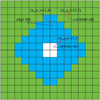 |
Fig. 1 Schematic view of a part of an ice layer in the partially active ice mantle. The blue, green, and white grids represent the edge, normal, and porous sites, respectively. |
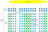 |
Fig. 2 Schematic diagram of our multiphase models in which pores exist in the ice mantle. The yellow area indicates the gas phase. The blue, green, red, and light blue balls represent species in the active layers, normal species, interstitial species, and edge layer species, respectively. Species in the active layers can diffuse into the edge layers. Species in the edge layers can also diffuse into the active layers. So, the active layers and edge layers are combined together to form bigger active layers. Normal species are frozen in the partially active ice mantle. |
Parameters in various models.
3 Results
In this section we report the abundances of major icy species in the cold core stage (Sec. 3.1), followed by the abundances of long carbon-chain species in the warming-up stage (Sec. 3.2). The abundances of JCH4 in the warming-up stage are also reported in the Sect. 3.2 because CH4 is crucial for the synthesis of long carbon-chain species in the lukewarm stage when the temperatures are around 30 K.
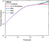 |
Fig. 3 Temporal evolution of JH2O fractional abundances predicted by models M01-M03, and by the two-phase and LCA multiphase models in the cold core stage. |
3.1 Major ice abundances in the cold core stage
Figure 3 shows the temporal evolution of JH2O fractional abundances predicted by different models in the cold core stage. The letter J designates icy species on grain surfaces. So, JH2O represents all H2O molecules in the active layers, interstitial sites, normal sites, and edge sites. The two-phase and LCA multiphase models respectively predicted the most and least abundant JH2O abundances among all models. The reason is as follows. Water ice is formed by the hydrogenation of JO, JO2, or JO3 in the models. In the two-phase model, almost all the JO2 and JO3 molecules are hydrogenated to form JH2O. Moreover, JH2O abundances can hardly be reduced by the photodissociation reactions in the two-phase model for the following reasons. The products of the JH2O photodissociation reaction are JOH and JH (or JO and JH). These species can form JH2O molecules again in the two-phase model, and so the JH2O abundance predicted by the two-phase model is the most abundant. In the porous multiphase models M01-M03 and the LCA multiphase model, however, JO2 and JO3 can be buried in the partially active ice mantle (Lu et al. 2018), and thus cannot be fully hydrogenated. Moreover, the photodissociation products of normal or interstitial JH2O (JO and JOH) can be locked in the partially active ice mantle in the form of radicals in these multiphase models. These radicals cannot efficiently form JH2O again in the multiphase models (Lu et al. 2018). Therefore, the JH2O abundances predicted by the multiphase models are lower than that predicted by the two-phase model. We can also see that JH2O abundances predicted by our porous multiphase models become closer to that by the two-phase models as α increases. On the other hand, the abundances of JH2O predicted by the models overall do not differ much (within a factor of 2).
Figure 4 shows the fractional abundances of JCO as a function of time predicted by different models in the cold core stage. The abundances of JCO predicted by different models are very similar before the time 105 yr; after the time 105 yr, minor differences arise. Model M03 predicts the highest JCO abundances among models M01-M03 at the time 3 × 10⁵ yr, followed by model M02. The abundance of JCO in Model M01 is the lowest at 3 × 10⁵ yr. This means that JCO molecules are easier to be hydrogenated as the α values used in the models increase. This trend can be explained as follows. Surface CO molecules are mainly destructed by hydrogenation reactions in our models in the cold core stage. They are mainly hydrogenated in the bigger active layers in models M01-M03 because there are few interstitial H atoms in the partially active ice mantles, and so the hydrogenation of JCO mainly occurs in the bigger active layers. More JCO molecules are available for hydrogenation in the bigger active layers as the α values used in the models increase. So, the calculated abundances of JCO decrease as the adopted α values in models increase. The LCA multiphase model predicts higher JCO abundances than models M01-M03 do because fewer JCO molecules are available for hydrogenation in the LCA multiphase model than in models M01-M03. All JCO molecules can be hydrogenated in the two-phase model; however, the two-phase model predicts higher JCO abundances than models M01 and M02 do at the time 3 × 10⁵ yr. The reason is that JO2 and JO3 molecules can also be hydrogenated in our models. The hydrogenation of JO2 and JO3 consumes JH atoms. All JO2 and JO3 molecules can be hydrogenated in the two-phase model, and so the JH abundance in the two-phase model is lower than that in models M01 and M02. Therefore, JCO molecules are less efficiently hydrogenated in the two-phase model than in models M01 and M02.
Figure 5 shows the fractional abundances of JCO2 and JCH4 as a function of time predicted by different models in the cold core stage. The differences in the JCO2 and JCH4 abundances predicted by these models are even smaller (within 50%). Hydrogenation reaction is the dominant reaction in which a species can participate because only H atoms can quickly diffuse in the cold stage. However, these two species cannot be further hydrogenated. Therefore, although H atoms can encounter them more frequently in the two-phase model than in the LCA multiphase model or in models M01-M03, the abundances of JCO2 and JCH4 in the two-phase model are similar to those in the four multiphase models. On the other hand, the abundances of JCO2 are about three orders of magnitude lower than those of JCO in all models. However, the abundances of JCO2 and JCO in cold cores should be comparable based on observations (Öberg et al. 2011). The discrepancy is discussed in Sect. 5.
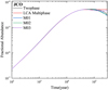 |
Fig. 4 Temporal evolution of JCO fractional abundances predicted by models M01-M03, and by the two-phase and LCA multiphase models in the cold core stage. |
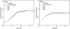 |
Fig. 5 Temporal evolution of JCO2 and JCH4 fractional abundances predicted by models M01-M03, and by the two-phase and LCA multiphase models in the cold core stage. |
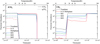 |
Fig. 6 Temporal evolution of the fractional abundances of CH4, JCH4, and gCH4 in models M01-M03, and in the two-phase and LCA multiphase models in the warming-up stage. |
3.2 Long carbon-chain species in the lukewarm stage
Figure 6 shows the fractional abundances of JCH4, gCH4, and CH4 as a function of time in the warming-up stage in models M01-M03, and in the two-phase and LCA multiphase models. The letter g designates sublimable icy species, which can sublime upon warming before JH2O molecules sublime (~110 K). Sublimable species are those in the active layers, edge sites, or interstitial sites in our models. Species in the normal sites are not sublimable species. The abundances of JCH4 in these five models are not much different at the time 3 × 10⁵ yr when the temperature is 10 K. However, the abundances of gCH4 in these models can be quite different. The two-phase model predicts the most abundant gCH4 molecules because all JCH4 molecules are sublimable in this model. The abundances of gCH4 predicted by models M01-M03 are higher than that by the LCA multiphase model because JCH4 molecules in the edge sites in models M01-M03 are also sublimable. Comparing gCH4 abundances in models M01-M03, we can see that model M01 predicts the most abundant gCH4 among these three porous multiphase models because model M01 has more edge sites than the other two models. Model M03 has fewer edge sites than models M01 and M02 do, and so it predicts the least abundant gCH4 among models M01-M03.
The abundances of gCH4 determine the abundances of gas-phase CH4 upon warming before JH2O molecules sublime in models. The two-phase model predicts the most abundant CH4. The CH4 abundance can be as high as 3.5 × 10⁻⁶ in the two-phase model. The LCA multiphase model predicts the least abundant CH4. The maximum fractional abundance of CH4 predicted by the LCA multiphase models is about 3.5 × 10⁻⁷, which is one order of magnitude lower than that by the two-phase model. In models M01-M03, the fractional abundances of CH4 before JH2O molecules sublime increase as α becomes larger. Model M01 predicts the highest CH4 abundances among these three porous multiphase models. The abundance of CH4 can reach a maximum of 1.7 × 10⁻⁶ in model M01. Although the maximum fractional abundance of CH4 predicted by model M01 is approximately half of that predicted by the two-phase model, it is more than a factor of 5 larger than that predicted by the LCA multiphase model. Model M03 predicts the lowest CH4 abundances. The maximum CH4 fractional abundance in model M03 is about 8 × 10⁻⁷.
Figure 7 shows the temporal evolution of the fractional abundances of four representative long carbon-chain species, C4H, C4H2, CH3CCH, and HC5N estimated by the two-phase, LCA multiphase and the porous multiphase models M01-M03. Synthesis of these long carbon-chain species in the lukewarm corinos requires CH4 as a precursor (Sakai et al. 2008, 2009a). This means that higher gas-phase CH4 abundances lead to higher long carbon-chain species abundances when the temperature is around 30 K. Therefore, the abundances of these four species are the highest in the two-phase model. Models M01-M03 predict less abundant long carbon-chain species than the two-phase model does (T ~ 30 K). The abundances of these species estimated by model M01 is typically a factor of 2 or 3 lower than that estimated by the two-phase model. The abundances of these long carbon-chain species predicted by models M01-M03 decrease as the α and rp values used in the models decrease. Long carbon-chain species abundances estimated by model M01 can be a factor of 5 larger than that by model M03, which typically estimates the lowest long carbon-chain species abundances. However, even model M03 can estimate much more abundant long carbon-chain species than the LCA multiphase model does when temperature is around 30 K. The abundances of long carbon-chain species predicted by model M03 are about a factor of 5 higher than these by the LCA multiphase model.
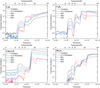 |
Fig. 7 Temporal evolution of the fractional abundances of selected carbon-chain species in models M01–M03, and in the two-phase and LCA multiphase models in the warming-up stage. |
4 Comparison with observations
We compare our model results with observations in this section. In order to quantitatively measure the agreement between our model results and observations, we utilized the mean confidence level approach (Garrod et al. 2007). In this approach, the confidence level (κj) is used to quantitatively measure the agreement between the abundance in a model (Xj) and the observed abundance of species j (Xobs,j). We calculated κj using the equation
![Mathematical equation: $\[\kappa_{\mathrm{j}}=\operatorname{erfc}\left(\frac{\left|\lg \mathrm{X}_{\mathrm{j}}-\lg \mathrm{X}_{\mathrm{obs}, \mathrm{j}}\right|}{\sqrt{2} \sigma}\right),\]$](/articles/aa/full_html/2024/11/aa50647-24/aa50647-24-eq9.png) (4)
(4)
where erfc is the complementary error function and σ is the standard error. The lowest value of κj is 0. The values of κj becomes larger as the agreement with the observations become better, but the value of κj cannot be more than 1. Following Garrod et al. (2007), we set the value σ = 1. The value of κj is 0.317 if the abundance of a species j in a model deviates from the observations by one order of magnitude. Moreover, we calculated the average κ for all the observed species in a source (![Mathematical equation: $\[\bar{\kappa}\]$](/articles/aa/full_html/2024/11/aa50647-24/aa50647-24-eq10.png) ). The value of
). The value of ![Mathematical equation: $\[\bar{\kappa}\]$](/articles/aa/full_html/2024/11/aa50647-24/aa50647-24-eq11.png) is time dependent. The time when
is time dependent. The time when ![Mathematical equation: $\[\bar{\kappa}\]$](/articles/aa/full_html/2024/11/aa50647-24/aa50647-24-eq12.png) takes the maximum value (κmax) is the optimum time (topt). We used κmax to quantify the global agreement between the observed and simulated abundances of species. At the time topt, we counted the number of molecules whose fractional abundance predicted by the models are within one order of magnitude of the observations. That number of molecules is the number of fits, which is another parameter for quantifying the global agreement. The temperature at the time topt is T (K)opt.
takes the maximum value (κmax) is the optimum time (topt). We used κmax to quantify the global agreement between the observed and simulated abundances of species. At the time topt, we counted the number of molecules whose fractional abundance predicted by the models are within one order of magnitude of the observations. That number of molecules is the number of fits, which is another parameter for quantifying the global agreement. The temperature at the time topt is T (K)opt.
Table B.1 shows the comparison between our model results and the observations toward the WCCC source L1527. We can see that the two-phase model no longer performs the best to predict the observed long carbon-chain species abundances. Instead, our porous multiphase model M01 performs the best to reconcile with observations based on the global agreement parameters. The κmax value for model M01 is 0.631, which is larger than that for the two-phase model (0.602). Moreover, the number of fits for the two-phase model is 21, which is smaller than that for model M01 (23). Comparing the three porous multiphase model results with observations, we found that the global agreement typically becomes worse as the α values used in the models become smaller. The κmax value drops from 0.631 to 0.530 as α decreases from 60% to 10%. The number of fits drops from 23 to 19 as α decreases. The LCA multiphase model performs the worst to reproduce the observed abundances of species toward L1527 because the values of κmax and the number of fits for the LCA multiphase model are the smallest. On the other hand, it is interesting to see that porous multiphase models M01 and M02 can predict CO abundance toward L1527 reasonably well. Finally, we can see that the two-phase model predicts the lowest T (K)opt (~30 K), while the LCA multiphase model predicts the highest T(K)opt (~34 K). Models M01-M03 estimate that T(K)opt values are between 31 K and 34 K.
Table B.2 shows the comparison between model results and observations toward the WCCC source B228. Among models M01-M03, model M01 performs the best to reproduce the observed species abundances. Model M01 overestimates two long carbon-chain species, C3H2 and C4H2, by more than one order of magnitude. The number of fits and κmax for models M01-M03 decrease as the α values used in models decrease. Models M02 and M03 underestimate the abundances of C4H, C3H2, and C4H2 by more than one order of magnitude, while the abundance of CH3CCH predicted by model M03 is more than one order of magnitude. The two-phase model also overestimates the abundances of C3H2 and C4H2 by more than one order of magnitude. However, the κmax value for the two-phase model is larger than that for model M01. The κmax value for the LCA multiphase model is smallest among all the models. This model underestimates C4H, CH3CCH, and HC5N by more than one order of magnitude. However, the LCA multiphase model can reproduce reasonably well the observed abundances of C3H2 and C4H2.
Table B.3 shows the comparison between model results and observations toward the WCCC source L483. We can see that models M01-M03 can reasonably well reproduce the observed abundances of species toward L483. The κmax values for models M01-M03 are all above 0.6. The number of fits for these models is no less than 15. The largest κmax value is that for model M02: 0.632. However, the number of fits for model M02 (15) is the smallest. Model M01 can estimate well the abundances of all long carbon-chain species: C4H, C3H2, HC3N and HC5N. The κmax value for model M01 is 0.628, which is only slightly less than that for model M02, and so we argue that model M01 performs the best to predict the observed abundances toward L483 among models M01-M03. The value of κmax and the number of fits for the two-phase model are all smaller than for models M01-M03. However, the two-phase model predicts the abundances of all four long carbon-chain species reasonably well. The LCA multiphase model still performs the worst to reproduce the observed abundances toward L483 among all models.
5 Discussions and conclusions
We proposed a porous multiphase model based on the LCA multiphase model and studied the formation of long carbon-chain species in the WCCC sources using this model. The porous structure of the ice mantle in our porous multiphase models enlarge the active layers, such that more JCH4 molecules can sublime upon warming. Gaseous CH4 is a precursor for the synthesis of long carbon-chain species in the gas-phase in the lukewarm stage. Therefore, the abundances of long carbon-chain species predicted by our porous multiphase models are higher than that by the LCA multiphase model. Moreover, as the porosity parameters α increases, long carbon-chain species abundances predicted by the porous multiphase models approach those estimated by the two-phase model. On the other hand, as α decreases the long carbon-chain species abundances predicted by the porous multiphase models approach the LCA multiphase model results. Therefore, the porous multiphase model can be viewed as a bridge model that connects the two-phase and LCA multiphase model.
Our comparisons with observations toward WCCC sources show that the porous multiphase model M01 performs better than the two-phase model to reproduce the abundances of observed species toward two WCCC sources, L1527 and L483. Moreover, model M01 performs almost as well as the two-phase model to reconcile with observations toward the WCCC source B228. Model M01 used a rather large α value (0.6). As the α values used in the porous multiphase models decrease, it usually becomes more difficult for the porous multiphase model results to reconcile with observations. Models M02 and M03 used smaller α values, and they do not perform as well as the two-phase model to reproduce the observed abundances of species toward L1527 and B228. However, all three of these porous multiphase models work better than the two-phase model to reproduce the abundances of species toward L483. Finally, porous multiphase models that adopted α ≥ 0.4 can outperform the LCA multiphase model to predict the abundances of species toward these three WCCC sources.
It is interesting to see that the two-phase model performs the best to predict the abundances of species toward B228, but it cannot compete with model M03, which used a rather small α value (0.1) to predict the abundances of species toward L483. Our qualitative explanations are as follows. The porosity of ice mantles in these three WCCC courses might be different. The porosity of ice mantles in B228 may be the highest, followed by L1527. The porosity of ice mantles in L483 may be the lowest. Because of the higher porosity of ice mantle in B228, almost all the species in the ice mantle may be mobile, and so the two-phase model performs the best for B228. On the other hand, because of the lower porosity of ice mantles in L483, a significant number of icy species are trapped inside the ice mantles, and therefore the two-phase model performs worse than all the porous multiphase models to reconcile with observations toward L483.
We compared the results of models M02, M04, and M05 in order to investigate how the pore parameters N and rp affect model results. We found that models M04 and M02 predict almost the same abundant long carbon-chain species in the lukewarm stage. Model M05 predicts lower long carbon-chain species abundances than model M02 does in the lukewarm stage. Based on the model results comparison, we argue that α is the most important parameter in our porous multiphase models. The pore size and rp cannot affect model results significantly if α is fixed. If N and rp affect model results significantly, it is because the value of α determined by both of them changes.
Our study suggests that the porosity of the ice mantle could strongly affect the chemical evolution of astronomical sources in the lukewarm stage. However, the porosity of ice mantles in astronomical sources is not well known. Garrod (2013b) studied the formation of the ice mantle using the off-lattice Monte Carlo method and found that ice mantles become more porous as the gas-phase density increases. However, the study only used a few surface species and chemical reactions due to the high computational cost of the numerical method. It is not clear whether the conclusion is still valid if more species and full surface chemical reaction network are used in the simulations.
In order to investigate the impact of the islands of bare grain surface on model results, we compared the results of models M02 and MN02. We found that at tcold the abundances of icy species predicted by model MN02 deviate from those by model M02 by less than 2%. Moreover, models M02 and MN02 predict almost the same abundance values of long carbon-chain species in the lukewarm stage (the difference is within 3%). Our simulation results show that the islands of bare grain surface are not likely to affect the model results significantly. On the other hand, the islands of bare grain surface were eliminated by an arbitrary assumption in model MN02. To eliminate these islands in a more rigorous approach, the off-lattice Monte Carlo method should be used (Garrod 2013b). However, to the best of our knowledge, the off-lattice Monte Carlo method has not yet been used to simulate a full gas-grain reaction network because of its high computational cost.
Laboratory studies showed that irradiation decreases ice porosity (Palumbo 2006; Raut et al. 2008; Palumbo et al. 2010). The decrease in ice mantle porosity reduces the amount of JCH4 molecules that can sublime in the lukewarm stage based on our porous multiphase model results, and thus an astronomical source is less likely to be a WCCC source if it is in a region where the radiation is higher. However, WCCC sources tend to be found in regions where the radiation is stronger (Higuchi et al. 2018; Lefloch et al. 2018). The contradiction may be resolved by recent theoretical studies about the effects of radiation on WCCC (Aikawa et al. 2020; Kalvāns 2021; Sun et al. 2024). Based on these theoretical studies, stronger radiation can boost the formation of long carbon-chain species in the gas phase. Therefore, stronger radiation does not always decrease WCCC activity. It is likely that the WCCC activity of an astronomical source can be enhanced by stronger radiation even if fewer JCH4 molecules sublime in the lukewarm stage. On the other hand, the theoretical studies did not consider the porous structure of ice mantles (Palumbo 2006; Raut et al. 2008; Palumbo et al. 2010). To better understand the effects of radiation on the WCCC activity, it is necessary to consider the decrease in ice mantle porosity due to stronger radiation in future astrochemical models.
In addition to the formation of long carbon-chain species in the lukewarm stage, we also studied the hydrogenation of JCO in the cold core stage in this work. We found that JCO molecules are typically hydrogenated more efficiently as the ice mantles become more porous. It is interesting to compare our findings with the crack model results (Awad et al. 2005). In the crack model the hydrogenation rate of JCO depends on k0nH′, where k0 is the rate coefficient of the reaction, JCO + JH → JHCO, while nH′ is the number density of JH. The density of JCO should decrease more slowly if a smaller k0nH′ value is used because JCO molecules are mainly destroyed by the reaction JCO + JH → JHCO in the crack model. However, the crack model results showed that JCO molecules are hydrogenated faster if smaller X/α′ and k0nH′ values are used (Awad et al. 2005). In the crack model, X measures the length of a unit crack (pore) side that is perpendicular to the crack, while α′ is the depth of the cracks. Assuming X is fixed, the ice surface area increases as α′ becomes larger (X/α′ decreases). Therefore, the crack model results showed that a larger surface area can enhance the JCO hydrogenation rate, which is consistent with our findings.
Carbon dioxide cannot be efficiently synthesized on grain surfaces in the cold core stage in all our models. The most efficient reaction by which JCO2 are formed is JCO + JOH → JCO2 + JH. Because JCO and JOH can hardly diffuse at 10 K, JCO2 cannot be efficiently synthesized. Previous models adopted the chain-reaction mechanism in order to enhance the production of JCO2 at 10 K (Garrod 2011; Chang & Herbst 2012). Based on the chain-reaction mechanism, JH and JO can react to form JOH. The newly formed JOH can immediately react with neighboring JCO to form JCO2. Thus, the formation of JCO2 does not rely on the diffusion of JOH or JCO if the chain-reaction mechanism is included in the models. Lu et al. (2018) found that the abundance of JCO2 can be as much as 10% of the water ice abundance in the cold core stage if the chain-reaction mechanism is included in the LCA multiphase models. We included the chain-reaction mechanism in model M02 (hereafter M02′). Model M02′ predicts that JCO2 abundances are about one-third of those of JCO in the cold core stage, which agrees reasonably well with observations (Öberg et al. 2011). Moreover, the abundances of long carbon-chain species predicted by model M02′ in the lukewarm stage deviate from those by model M02 by less than 2%.
Although we did not study deuteration in this work, the porous multiphase model seems to be very promising for studying deuteration. It was found that the major problem with the GRAINOBLE model is that too many CO and N2 molecules are buried inside the ice mantle, and so gas-phase species deuteration predicted by the multiphase model fails to reconcile with observations (Sipilä et al. 2016). The LCA multiphase model results in this work confirmed the findings by Sipilä et al. (2016) because it underestimates CO abundance toward L1527 by more than one order of magnitude. Our porous multiphase models no longer underestimate CO abundances. The abundance of CO predicted by models M01 and M02 agree reasonably well with observations toward L1527. In a subsequent paper, we will report on deuteration studied using our porous multiphase models.
In addition to solving the problem that too many volatile molecules are trapped inside ice mantles, our porous multiphase models still predict much higher COM abundances than the two-phase model does. For instance, the abundance of CH3OCH3 at t = 5 × 10⁵ yr in M02 is 1.2 × 10⁻⁸, which is more than one order of magnitude higher than that in the two-phase model. Moreover, the CH3OCH3 abundance predicted by model M02 is only about a factor of 3 less than that by the LCA multiphase model (3.3 × 10⁻⁸). Therefore, the porous multiphase models are not likely to severely underestimate COM abundances. In a following paper we will report the study of COM formation in hot cores using the porous multiphase models.
For many years, astrochemists have been improving their chemical models in order to better estimate the abundances of species in astronomical sources. The choice of a two-phase or multiphase model remains a difficult problem because both models are supported by observational or laboratory evidence. In the current literature, both types of models are adopted for astrochemical modeling. This work suggests that both types of models may be suitable depending on the porosity of the ice mantle and the physical conditions of the sources. If the ice mantle is highly porous and the purpose is to study the gas-phase species in the lukewarm stage (~30 K), a simple two-phase model should be appropriate. The high porosity ensures that the majority of the species in the ice mantle can diffuse and sublime in the lukewarm stage, which is what the two-phase model assumes. The LCA or GRAINOBLE multiphase models do not work in this case because too many species are locked inside the ice mantle in these multiphase models. On the other hand, if the porosity of ice mantles in astronomical sources is so low that the majority of icy species are trapped in the ice mantles, multiphase models that do not consider the porous ice structure should be suitable for the astrochemical modeling of these sources.
Acknowledgements
The research was funded by The National Natural Science Foundation of China under grants 12173023 and 12203091. We thank Jiao He, Jingfei Sun and Yao Wang for helpful discussions. We thank Yang Lu for providing the LCA multiphase model Monte Carlo codes. We thank our referee for careful reading the manuscript and providing constructive comments to improve the quality of paper.
Appendix A The porous model
Here we provide a more complete description of our porous multiphase models. Our porous multiphase models have the following rules and constraints.
(1) The ice mantle on a dust is divided into two parts, active layers and a partially active ice mantle.
(2) Sites in the ice mantle are classified into five types: sites in the active layers, normal sites, interstitial sites, edge sites, and porous sites. The sites in the active layers, the normal and interstitial sites already exist in the LCA multiphase model. We refer to Lu et al. (2018) for the details of them. A fraction of normal sites in the LCA multiphase model become porous or edge sites in our porous multiphase models. The porous sites are sites that always remain empty. Edge sites are sites surrounding the porous sites. They are defined as the follows. If the distance between a normal site in the LCA multiphase model and its nearest porous site is less or equal to four, the normal site is an edge site. Species occupying the edge sites can also diffuse or desorb.
(3) In the beginning of simulations, there is no icy species on the dust surfaces. Icy species population increase due to the accretion of gas-phase species. Icy species fill sites in the active layers first. The maximum population of icy species in the active layers are four monolayers.
(4) Pores are formed as the partially active ice mantles gradually build up layer by layer. The partially active ice mantles are formed due to the addition of icy species to the active layers that already reach their maximum capacity. If an icy species A is added to active layers with four monolayers of species, a species B is randomly chosen from the active layers. The species B is put in the ice layers that are underneath the active layers. The species B occupies the edge sites first. After all edge sites in the layer are occupied, the species B fills the normal sites in the layer. We adopt the method described by Vasyunin & Herbst (2013) to fill the normal sites with icy species. After all non-porous sites in the layer are occupied by icy species, non-porous sites in another layer start to be filled. The ice mantles then gradually build up layer by layer. Because porous sites always remain empty, pores are formed as the ice mantle builds up layer by layer.
(5) Species in the edge sites form edge layers. Species in the edge layers can diffuse as fast as they do in the active layers. The hopping rate of species i in the active or edge layers is, ![Mathematical equation: $\[\mathrm{k}_{\mathrm{hop}, \mathrm{i}}=\nu \exp \left(\frac{-\mathrm{E}_{\mathrm{bli}}}{\mathrm{T}}\right)\]$](/articles/aa/full_html/2024/11/aa50647-24/aa50647-24-eq13.png) where T is the temperature while ν = 1012 s−1 is the attempt frequency. The edge layers interconnect with the active layers. Species in the active layers can diffuse into the edge layers. Species in the edge layers can also diffuse into the active layers. However, we do not explicitly simulate these two processes in the porous multiphase models. Instead, we combine the edge layers and the active layers to form bigger active layers. Species can diffuse in the bigger active layers as they do in the active layers.
where T is the temperature while ν = 1012 s−1 is the attempt frequency. The edge layers interconnect with the active layers. Species in the active layers can diffuse into the edge layers. Species in the edge layers can also diffuse into the active layers. However, we do not explicitly simulate these two processes in the porous multiphase models. Instead, we combine the edge layers and the active layers to form bigger active layers. Species can diffuse in the bigger active layers as they do in the active layers.
(6) Volatile species in the bigger active layers sublime when the temperature is higher than their sublimation temperatures. The ice mantles desorb layer by layer as the follows in our models. After a species, i, leaves the bigger active layers, we check the number of normal species in the ice layer that is immediately adjacent to the active layers (IAA ice layer), Nnor. If Nnor > 0, following the approach in Vasyunin & Herbst (2013), we randomly chose a normal species in the IAA ice layer and placed it in the bigger active layers. If Nnor is 0, the number of edge species in the IAA ice layer is reduced by one. After all species in the IAA ice layer leave, the ice layer that is immediately adjacent to the IAA layer becomes a new IAA ice layer. Icy species then start to leave the new IAA layer due to the desorption of species in the bigger active layers.
(7) Two-body reactions occur due to the diffusion of species in the bigger active layers. The reaction rate coefficient for a two-body reaction between species i and j is
![Mathematical equation: $\[\mathrm{r_{i j}}=\frac{\mathrm{k}_{\text {hop }, \mathrm{i}}+\mathrm{k}_{\text {hop }, \mathrm{j}}}{\left(1-\mathrm{r}_{\mathrm{p}}\right) \mathrm{N}_{\mathrm{s}}+\mathrm{N}_{\mathrm{L}} \mathrm{~N}_{\mathrm{ed}} \mathrm{~N}_{\mathrm{s}} \mathrm{r}_{\mathrm{p}} / \mathrm{N}},\]$](/articles/aa/full_html/2024/11/aa50647-24/aa50647-24-eq14.png) (A.1)
(A.1)
where khop,j is the hopping rate of species j while Ned is the number of edge sites that are immediately adjacent to the porous sites of a pore at each ice layer. As defined in the main text, N is the pore size, Ns is total number of normal sites, edge sites and porous sites while NL is the number of ice layers in the partially active ice mantle. For a 3 × 3 pore, Ned = 16. The denominator of Eqn. A.1 represents the number of sites species i and j should visit before they encounter in the bigger active layers.
(8) Normal species are trapped in the partially active ice mantle while interstitial species can diffuse at a slower rate compared to species in the bigger active layers. The diffusion of interstitial species can lead to two-body reactions between interstitial species. Two-body reactions between interstitial and normal specie can also occur due to the diffusion of interstitial species. The reaction rate coefficients for these two type of reactions have been explained in detail in Lu et al. (2018). We adopted these rate coefficients in the porous multiphase models.
(9) Interstitial species can diffuse into the bigger active layers. They diffuse into the active layers or edge layers with different rate coefficients. The rate coefficient for an interstitial species j to diffuse into the active layers is (Lu et al. 2018)
![Mathematical equation: $\[\mathrm{r_{n 1 j}}=\frac{\mathrm{k}_{\text {hop}, \mathrm{j}}}{6} \frac{\mathrm{N_j}}{\mathrm{N_L}},\]$](/articles/aa/full_html/2024/11/aa50647-24/aa50647-24-eq15.png) (A.2)
(A.2)
where Nj is the population of interstitial species j. Following the method adopted by Lu et al. (2018) to derive Eqn. A.2, we found the rate coefficient for an interstitial species j to diffuse into the edge layers is
![Mathematical equation: $\[\mathrm{r_{n 2 j}}=\left(\frac{\mathrm{N_n}-4 \sqrt{\mathrm{N}}}{3}+\frac{4 \sqrt{\mathrm{N}}}{6}\right) \frac{\mathrm{k}_{\text {hop,j}} \mathrm{r_p}}{\mathrm{N}\left(1-\alpha-\mathrm{r_p}\right)},\]$](/articles/aa/full_html/2024/11/aa50647-24/aa50647-24-eq16.png) (A.3)
(A.3)
where Nn is the number of normal sites that are immediately adjacent to the edge sites at each ice layer. For a 3 × 3 pore, Nn = 28. So, the rate coefficient that an interstitial species j diffuse into the bigger active layers is rnj = rn1j + rn2j.
(10) Photons can penetrate into the ice mantle layer by layer and photodissociate icy species. The photodissociation of normal and interstitial species in our model follows the rules in Lu et al. (2018).
Appendix B Additional tables
Comparison of model results with observations toward L1527.
Comparison of the simulated and the observed fractional abundances of species toward B228.
Simulated and observed fractional abundances of species toward L483.
References
- Awad, Z., Chigai, T., Kimura, Y., Shalabiea, O. M., & Yamamoto, T. 2005, ApJ, 626, 262 [NASA ADS] [CrossRef] [Google Scholar]
- Aikawa, Y., Wakelam, V., Garrod, R. T., & Herbst, E. 2008, ApJ, 674, 993 [Google Scholar]
- Aikawa, Y., Furuya, K., Yamamoto, S., & Sakai, N. 2020, ApJ, 897, 110 [Google Scholar]
- Andersson, S., & van Dishoeck, E. F. 2008, A&A, 491, 90 [Google Scholar]
- Agúndez, M., Cernicharo, J., & Guéli, M. 2015, A&A, 577, L5 [NASA ADS] [CrossRef] [EDP Sciences] [Google Scholar]
- Benson, P. J., Caselli, P., & Myers, P. C. 1998, ApJ, 506, 743 [Google Scholar]
- Biham, O., Furman, I., Pirronello, V., & Vidali G. 2001, ApJ, 553, 595 [NASA ADS] [CrossRef] [Google Scholar]
- Boogert, A. A., Gerakines, P. A., & Whittet, D. C. 2015, ARA&A, 53, 541 [NASA ADS] [CrossRef] [Google Scholar]
- Chang, Q., & Herbst, E. 2012, ApJ, 759, 147 [Google Scholar]
- Chang, Q., & Herbst, E. 2014, ApJ, 787, 135 [Google Scholar]
- Chang, Q., Cuppen, H., & Herbst, E. 2005, A&A, 434, 599 [NASA ADS] [CrossRef] [EDP Sciences] [Google Scholar]
- Chang, Q., Lu, Y., & Quan D. 2017, ApJ, 851, 68 [NASA ADS] [CrossRef] [Google Scholar]
- Carmack, R. A., Tribbett, P. D., & Loeffler, M. J. 2023, ApJ, 942, 1 [NASA ADS] [CrossRef] [Google Scholar]
- Collings, M. P., Dever, J. W., Fraser, H. J., McCoustra, M. R. S., & Williams, D. A. 2003, ApJ, 583, 1058 [NASA ADS] [CrossRef] [Google Scholar]
- Furuya, K., Aikawa, Y., Hincelin, U., et al. 2015, A&A, 584, A124 [NASA ADS] [CrossRef] [EDP Sciences] [Google Scholar]
- Garrod, R. 2013a, ApJ, 765, 60 [CrossRef] [Google Scholar]
- Garrod, R. 2013b, ApJ, 778, 158 [CrossRef] [MathSciNet] [Google Scholar]
- Garrod, R., & Herbst, E. 2006, A&A, 457, 927 [NASA ADS] [CrossRef] [EDP Sciences] [Google Scholar]
- Garrod, R., & Pauly, T. 2011, ApJ, 735, 15 [NASA ADS] [CrossRef] [Google Scholar]
- Garrod, R., Wakelam, V., & Herbst, E. 2007, A&A, 467, 1103 [NASA ADS] [CrossRef] [EDP Sciences] [Google Scholar]
- Gibb, E. L., Whittet, D. C. B., Boogert, A. C. A., & Tielens, A. G. G. M. 2004, ApJS, 151, 35 [NASA ADS] [CrossRef] [Google Scholar]
- Hasegawa, T. I., Herbst, E., & Leung, C. M. 1992, ApJS, 82, 167 [Google Scholar]
- Hassel, G. E., Herbst, E., & Garrod, R. 2008, ApJ, 681, 1385 [NASA ADS] [CrossRef] [Google Scholar]
- Higuchi, A. E., Sakai, N., Watanabe, Y., et al. 2018, ApJS, 236, 52 [Google Scholar]
- Hirota, T., Ohishi, M., & Yamamoto, S. 2009, ApJ, 699, 585 [Google Scholar]
- Jørgensen, J. K., Schöier, F. L., & van Dishoeck, E. F. 2002, A&A, 389, 908 [CrossRef] [EDP Sciences] [Google Scholar]
- Jørgensen, J. K., Schöier, F. L., & van Dishoeck, E. F. 2004, A&A, 416, 603 [Google Scholar]
- Jørgensen, J. K., Belloche, A., & Garrod, R. 2020, ARA&A, 58, 727 [CrossRef] [Google Scholar]
- Kalvāns, J. 2015, ApJ, 803, 52 [CrossRef] [Google Scholar]
- Kalvāns, J. 2021, ApJ, 910, 54 [CrossRef] [Google Scholar]
- Lefloch, B., Bachiller, R., Ceccarelli, C., et al. 2018, MNRAS, 477, 4792 [Google Scholar]
- Lu, Y., Chang, Q., & Aikawa, Y. 2018, ApJ, 869, 165 [Google Scholar]
- Molinari, S., Brand, J., Cesaroni, R., & Palla, F. 2000, A&A, 355, 617 [NASA ADS] [Google Scholar]
- Öberg, K., Boogert, A. C. A., Pontoppidan, K. M., et al. 2011, ApJ, 740, 109 [CrossRef] [Google Scholar]
- Palumbo, M. E. 2006, A&A, 453, 903 [NASA ADS] [CrossRef] [EDP Sciences] [Google Scholar]
- Palumbo, M. E., Baratta, G. A., Leto, G., & Strazzulla, G. 2010, J. Mol. Struct., 972, 64 [NASA ADS] [CrossRef] [Google Scholar]
- Pickles, J. B., & Williams, D. A. 1977, Ap&SS, 52, 443 [NASA ADS] [CrossRef] [Google Scholar]
- Raut, U., Famá, M., Loeffler, M. J., & Baragiola, R. A. 2008, ApJ, 687, 1070 [NASA ADS] [CrossRef] [Google Scholar]
- Sakai, N., Sakai, T., Hirota, T., & Yamamoto, S. 2008, ApJ, 672, 371 [Google Scholar]
- Sakai, N., Sakai, T., Hirota, T., Burton, M., & Yamamoto, S. 2009a, ApJ, 702, 1025 [NASA ADS] [CrossRef] [Google Scholar]
- Sakai, N., Sakai, T., Hirota, T., Burton, M., & Yamamoto, S. 2009b, ApJ, 697, 769 [Google Scholar]
- Sakai, N., Shirley, Y. L., Sakai, T., et al. 2012, ApJ, 758, L4 [NASA ADS] [CrossRef] [Google Scholar]
- Sandford, S. A., & Allamandola, L. J. 1988, Icar, 76, 201 [NASA ADS] [CrossRef] [Google Scholar]
- Sipilä, O., Caseli, P., & Taquet, V. 2016, A&A, 591, A9 [NASA ADS] [CrossRef] [EDP Sciences] [Google Scholar]
- Sun, J., Li, X., Du, F., et al. 2024, A&A, 683, A76 [NASA ADS] [CrossRef] [EDP Sciences] [Google Scholar]
- Tafalla, M., Myers, P. C., Mardones, D., & Bachiller, R. 2000, A&A, 359, 967 [NASA ADS] [Google Scholar]
- Taquet, V., Ceccarelli, C., & Kahane, C. 2012, A&A, 538, A42 [NASA ADS] [CrossRef] [EDP Sciences] [Google Scholar]
- Tielens, A. G. G. M., Tokunaga, A. T., Geballe, T. R., & Baas, F. 1991, ApJ, 381, 181 [NASA ADS] [CrossRef] [Google Scholar]
- Vasyunin, A. I., & Herbst, E. 2013, ApJ, 762, 86 [Google Scholar]
- Vasyunin, A. I., Semenov, D. A., Wiebe, D. S., & Henning, T. 2009, ApJ, 691, 1459 [Google Scholar]
- Vasyunin, A. I., Caselli, P., Dulieu, F., & Jiménez-Serra, I. 2017, ApJ, 842, 33 [Google Scholar]
- Wang, Y., Chang, Q., & Wang, H. 2019, A&A, 622, A185 [NASA ADS] [CrossRef] [EDP Sciences] [Google Scholar]
All Tables
Comparison of the simulated and the observed fractional abundances of species toward B228.
All Figures
|
Fig. 1 Schematic view of a part of an ice layer in the partially active ice mantle. The blue, green, and white grids represent the edge, normal, and porous sites, respectively. |
| In the text | |
|
Fig. 2 Schematic diagram of our multiphase models in which pores exist in the ice mantle. The yellow area indicates the gas phase. The blue, green, red, and light blue balls represent species in the active layers, normal species, interstitial species, and edge layer species, respectively. Species in the active layers can diffuse into the edge layers. Species in the edge layers can also diffuse into the active layers. So, the active layers and edge layers are combined together to form bigger active layers. Normal species are frozen in the partially active ice mantle. |
| In the text | |
|
Fig. 3 Temporal evolution of JH2O fractional abundances predicted by models M01-M03, and by the two-phase and LCA multiphase models in the cold core stage. |
| In the text | |
|
Fig. 4 Temporal evolution of JCO fractional abundances predicted by models M01-M03, and by the two-phase and LCA multiphase models in the cold core stage. |
| In the text | |
|
Fig. 5 Temporal evolution of JCO2 and JCH4 fractional abundances predicted by models M01-M03, and by the two-phase and LCA multiphase models in the cold core stage. |
| In the text | |
|
Fig. 6 Temporal evolution of the fractional abundances of CH4, JCH4, and gCH4 in models M01-M03, and in the two-phase and LCA multiphase models in the warming-up stage. |
| In the text | |
|
Fig. 7 Temporal evolution of the fractional abundances of selected carbon-chain species in models M01–M03, and in the two-phase and LCA multiphase models in the warming-up stage. |
| In the text | |
Current usage metrics show cumulative count of Article Views (full-text article views including HTML views, PDF and ePub downloads, according to the available data) and Abstracts Views on Vision4Press platform.
Data correspond to usage on the plateform after 2015. The current usage metrics is available 48-96 hours after online publication and is updated daily on week days.
Initial download of the metrics may take a while.