| Issue |
A&A
Volume 689, September 2024
|
|
|---|---|---|
| Article Number | A325 | |
| Number of page(s) | 9 | |
| Section | Interstellar and circumstellar matter | |
| DOI | https://doi.org/10.1051/0004-6361/202450539 | |
| Published online | 23 September 2024 | |
Argon X-ray absorption in the local interstellar medium
1
Max-Planck-Institut für extraterrestrische Physik, Gießenbachstraße 1, 85748 Garching, Germany
2
Department of Physics, Western Michigan University, Kalamazoo, MI 49008, USA
3
Department of Computer Engineering, Hasan Kalyoncu University, 27100 Sahinbey, Gaziantep, Turkey
4
NASA Goddard Space Flight Center, Greenbelt, MD 20771, USA
Received:
29
April
2024
Accepted:
4
August
2024
Abstract
We present the first comprehensive analysis of the argon K-edge absorption region (3.1–4.2 Å) using high-resolution HETGS Chandra spectra of 33 low-mass X-ray binaries. Utilizing R-matrix theory, we computed new K photoabsorption cross sections for Ar I–Ar XVI species. For each X-ray source, we estimated column densities for the Ar I, Ar II, Ar III, Ar XVI, Ar XVII, and Ar XVIII ions, which trace the neutral, warm, and hot components of the gaseous Galactic interstellar medium. We examined their distribution as a function of Galactic latitude, longitude, and distances to the sources. However, no significant correlations were discerned among distances, Galactic latitude, or longitude. Future X-ray observatories will allow us to benchmark the atomic data as the main resonance lines will be resolved.
Key words: ISM: atoms / ISM: structure / local insterstellar matter / X-rays: ISM
Corresponding author; This email address is being protected from spambots. You need JavaScript enabled to view it.
© The Authors 2024
 Open Access article, published by EDP Sciences, under the terms of the Creative Commons Attribution License (https://creativecommons.org/licenses/by/4.0), which permits unrestricted use, distribution, and reproduction in any medium, provided the original work is properly cited.
This article is published in open access under the Subscribe to Open model.
Open Access funding provided by Max Planck Society.
1 Introduction
The interstellar medium (ISM) stands as a fundamental constituent in Galactic dynamics, influencing star life cycles and regulating cooling processes in molecular clouds, which enables star formation (Wong & Blitz 2002; Bigiel et al. 2008; Leroy et al. 2008; Lada et al. 2010; Lilly et al. 2013). Comprising gas and dust dispersed between stars, the ISM manifests in multiple phases characterized by distinct gas temperatures spanning from 10 to 106 K (e.g., McKee & Ostriker 1977; Falgarone et al. 2005; Tonnesen & Bryan 2009; Draine 2011; Jenkins & Tripp 2011; Rupke & Veilleux 2013; Zhukovska et al. 2016; Stanimirović & Zweibel 2018).
High-resolution X-ray spectroscopy emerges as a potent tool for dissecting the complex environment of the ISM. This analytical technique requires bright X-ray sources functioning akin to beacons. By modeling absorption features discerned in X-ray spectra, we can study the physical properties of the intervening gas along the line of sight to the source. The advent of X-ray observatories equipped with grating spectrometers capable of high-resolution spectra has propelled ISM X-ray absorption studies to the forefront of X-ray astronomy. These investigations encompass the study of K photoabsorption edges across various elemental species such as O, Fe, Ne, Mg, N, Si, and S (Pinto et al. 2010, 2013; Costantini et al. 2012; Gatuzz et al. 2013b,a, 2014, 2015, 2016, 2018a,b, 2019, 2020b, 2021, 2023a,b; Joachimi et al. 2016; Gatuzz & Churazov 2018; Rogantini et al. 2018, 2021; Zeegers et al. 2019; Psaradaki et al. 2020; Yang et al. 2022). Furthermore, L-edge studies of Fe have also been carried out in the last decade (Costantini et al. 2012; Westphal et al. 2019; Psaradaki et al. 2023, 2024; Corrales et al. 2024).
Argon holds significant importance within the ISM due to its abundance and ability to trace various physical and chemical processes. Notably, argon serves as a diagnostic tool in shock regions, aiding in studying shock wave interactions within supernova remnants (Dopita et al. 2018, 2019). Its depletion onto dust grains influences the composition and properties of interstellar dust, thereby impacting processes such as dust grain growth (Arendt et al. 2014; Amayo et al. 2021; Jones et al. 2023). Furthermore, argon acts as a tracer of cosmic ray ionization in the ISM, contributing to our understanding of cosmic ray propagation and their effects on the surrounding medium (Ogliore et al. 2009). Observations of argon emission lines in star-forming regions help identify mechanisms triggering star formation (López-Sánchez & Esteban 2010; Strom et al. 2023). Additionally, the abundance of argon relative to other elements, such as hydrogen and oxygen, provides valuable information for studying the metallicity of different regions within the ISM (Hua et al. 2023). In comparison with studies of oxygen and sulfur, the amount of argon depletion into dust grains is more challenging. In their calculation of ionization correction factors for argon in giant H II regions, Amayo et al. (2021) provide only a qualitative analysis of the depletion into dust, given that argon stellar abundances are highly uncertain. Furthermore, although argon is mainly produced by core-collapse supernovae, Type Ia supernova may also contribute to its production (Seitenzahl et al. 2013; Leung & Nomoto 2018). In the Galactic chemical evolution by Kobayashi et al. (2020), they found that up to 34% of the argon in the solar vicinity can have a type Ia supernova origin. Therefore, studies of argon depletion onto dust must include chemical evolution models considering both supernova yields, despite their uncertainties Palla (2021).
In this study, we analyzed the Ar K-edge absorption region utilizing Chandra observations of low-mass X-ray binaries (LMXBs). Section 2 outlines the data sample and the spectral fitting procedure employed. Section 3 delves into the computation of atomic data and the incorporation of photoabsorption cross sections within our modeling framework. The outcomes of our fits are discussed in Sect. 4. Finally, Sect. 5 provides a concise summary of our analysis.
Galactic observations analyzed.
2 Data reduction and analysis
We analyzed Chandra spectra from 33 LMXBs observed along various lines of sight. Our sample selection criteria required a minimum of 1000 counts in the argon edge absorption region (3.1–4.2 Å). This criterion has been applied in previous analysis (e.g., Gatuzz et al. 2021, 2023a,b) and allows us to gather a diverse sample of sight lines, without preconceived assumptions about the strength of Argon absorption. While the column density (N(HI + H2)) is an important factor in X-ray transmission and absorption, imposing a constraint based on N(HI + H2) could introduce biases by preferentially selecting sight lines with certain characteristics. Our approach, based on counts, includes a wider range of column densities and a larger number of sources, therefore providing a more representative sample of the ISM conditions. We deliberately avoided biasing the sample by refraining from imposing constraints based on specific line detections, such as Ar XVII Kα.
Table 1 provides specifications for the selected sources, including Galactic coordinates, hydrogen column densities adopted from Willingale et al. (2013), and, when available, distances. Although the column densities from Willingale et al. (2013) represent average values of N(HI + H2) along sight lines traversing the entire Galaxy, these values are appropriate for our analysis due to the narrow wavelength region covered (~1 Å). Appendix A shows the observation IDs analyzed for each source.
All spectra were acquired using the High Energy Grating (HEG) in combination with the Advanced CCD Imaging Spectrometer (ACIS) on board Chandra. Data reduction procedures, including background subtraction, were performed using the Chandra Interactive Analysis of Observations (CIAO1, version 4.15.1), following the standard CIAO procedure for point-like sources. We used the findzo algorithm2 to estimate the zero-order position of those sources for which zero-order data were not telemetered. Then, we used the chandra_repro script, which reads data from the standard data distribution (e.g., primary and secondary directories) and creates a new bad pixel file together with an event file and type II PHA files, response files, and auxiliary response files.
The spectral fitting was conducted within the 3.1–4.2 Å wavelength range using the XSPEC package (version 12.11.13). We employed a powerlaw model to characterize the continuum, with parameters such as γ and normalization treated independently across all observations to accommodate potential variations over different epochs. The goodness-of-fit assessment utilized χ2 statistics, complemented by the weighting method proposed by Churazov et al. (1996).
Energies (in Rydbergs) for the Ar I ground state and the Ar II target states.
3 Photoabsorption cross section calculations
In order to fit the Ar K-edge absorption region, atomic Ar I-Ar XVI cross sections were computed by using R-matrix theory. Within a single-configuration perspective for the K-shell photoexcitation processes in the argon ground state, the following configurations were involved:
![Mathematical equation: $hv + S\left( {1{{\rm{s}}^2}2{{\rm{s}}^2}2{{\rm{p}}^6}3{{\rm{s}}^2}3{{\rm{p}}^6}} \right)\left[ {^1{\rm{S}}} \right] \to 1{\rm{s}}2{{\rm{s}}^2}2{{\rm{p}}^6}3{{\rm{s}}^2}3{{\rm{p}}^6}{\rm{np}}\left[ {^1{{\rm{P}}^o}} \right].$](/articles/aa/full_html/2024/09/aa50539-24/aa50539-24-eq8.png)
Using these orbitals, and some additional pseudoorbitals that were optimized on the 1 s-vacancy states and accounted for relaxation effects, the following list of target states and computed R-matrix energies were compared to available NIST values (see Table 2). The 2p−1 L-edge states are autoionizing themselves and are not available from the NIST atomic database (Kramida et al. 2020).
Those high-energy intermediate autoionizing states can decay via two fundamentally distinct Auger pathways. The first decay route is via participator Auger decay in which the valence electron, np, primarily takes part in the autoionization process,

yielding a decay rate that scales as 1/n3. The second decay pathway is spectator Auger decay in which the valance electron, np, does not take part in the autoionization process,

for which the Auger rate is independent of n. Spectator Auger decay becomes the dominant decay pathway at higher n values in the photoexcitation process and becomes constant at all n, leading to a significant broadening of entire Rydberg series of resonances below the K-edge and an apparent K-edge significantly below the actual K-shell ionization thresholds. In the standard R-matrix implementation (Burke 2011; Berrington et al. 1995), participant Auger decay is explicitly taken into account by including all final ArI I target states.
For spectator Auger, on the other hand, it is impossible to include all of the infinite 1s22ℓc3ℓdnp + e−, (c + d = 14) decay channels implicitly to account for spectator Auger decay effects within the standard R-matrix implementation. Instead, the present calculations utilized the modified R-matrix method to account for spectator Auger broadening effects by using an optical potential, as was described by Gorczyca & Robicheaux (1999); Burke (2011). In this approach, the target energy of each closed channel is modified, within a multi-channel quantum defect theory approach, as

where Γ is the 1s2s22p63s23p6 Auger width.
The Auger widths needed to treat spectator Auger broadening effects in 1s−1 autonionizing target states were computed by using the Wigner time delay method (Smith 1960). Specifically, the R-matrix method was employed on the e− + 1s2nℓq−2 scattering problem, similar to photoabsorption calculations in terms of basis set and configuration lists. Auger widths were then obtained by analyzing scattering channels. The Auger width for the 1s2s22p63s23p6 autonionizing state was determined to be 3.90 × 10⁻² Ryd. This modified R-matrix method with pseu-doresonance elimination (Gorczyca et al. 1995) was applied to all Ar I-Ar XIV ions, similar to earlier benchmarking with experimental synchrotron measurements (Gorczyca & Robicheaux 1999; Gorczyca & McLaughlin 2000; Gorczyca et al. 2013; Gorczyca 2000; Hasoglu et al. 2010) and high-resolution spectroscopic observations (Hasoglu et al. 2010; Hasoğlu et al. 2014; Gatuzz et al. 2020b, 2023b).
In order to account for relaxation effects due to 1s-vacancy, the orbital basis used in the implementation of R-matrix calculations consisted of physical orbitals and peseudoorbitals. For the present study, the number of electrons in the target states ranges from N = 0, 1, …, 10, and the orbitals consisted of 1s, 2s, and 2p physical orbitals and  pseudoorbitals. For N ≥ 10, a larger basis is needed to treat n = 3 resonances accurately. Therefore, 1s, 2s, 2p, 3s, and 3p were treated as physical orbitals and
  as pseudoorbitals. A Hartree-Fock method was employed to compute the physical orbitals. On the other hand, the pseudoorbitals, which are optimized to account for important orbital relaxation effects, were computed by utilizing a multi-configuration Hartree-Fock method on the configuration lists n = 3-complex (N < 10) and n = 4-complex (N ≥ 10) formed by single- and double-promotions from the 1s-vacancy configuration.
To characterize X-ray absorption in the ISM due to argon Ar, we utilized the photoabsorption cross sections for Ar I, Ar II, Ar III, and Ar XVI K-edge, as was previously described. Additionally, we incorporated the photoabsorption cross sections for Ar XVII and Ar XVIII from Witthoeft et al. (2011). These cross sections are depicted in Fig. 1 and integrated into a modified version of the ISMabs model (Gatuzz et al. 2015)4. The column densities of atomic hydrogen (HI) in ISMabs are constrained to the values provided by Willingale et al. (2013) for each source. For comparison, we also included Ar I cross section from Verner et al. (1996) and the Ar II, Ar III, Ar XVI cross sections from Witthoeft et al. (2011). The Verner et al. (1996) cross section does not include any resonance lines, only the K-edge. We note that for previously reported K-absorption cross sections of Argon ionized species computed by Witthoeft et al. (2011) while utilizing a similar R-matrix approach with the inclusion of Auger broadening, important orbital relaxation effects were not included because the single-electron orbitals were obtained by using a Thomas-Fermi-Dirac statistical model potential. Relaxation effects affect K-shell threshold estimation, as is shown by the overestimation by ~7 eV of the Ar II and Ar III K-edges. For instance, Fig. 2 illustrates the best fit achieved for the LMXB 4U 1916-053. Due to the nominal HEG resolution of Δλ ~ 12 mÅ, surpassing the separation of the Kα resonance lines, a detailed benchmarking of atomic data proves challenging. This limitation suggests a potential for future analyses leveraging high-resolution X-ray instrumentation (see Sect. 4.2).
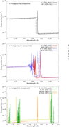 |
Fig. 1 Photoabsorption cross sections included in the model for Ar I (top panel), Ar II, Ar III (middle panel), Ar XVI, Ar XVII, and Ar XVIII (bottom panel). The plots also include an Ar I cross section from Verner et al. (1996) and Ar II, Ar III, and Ar XVI cross sections from Witthoeft et al. (2011). |
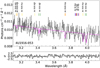 |
Fig. 2 Best-fit results in the Ar K-edge photoabsorption region for the LMXB 4U 1916-053. Black points correspond to the observation in flux units, while the red line corresponds to the best-fit model. Residuals are included in units of (data − model)/error. The position of the Kα absorption lines are indicated for each ion, following the color code used in Fig. 1. |
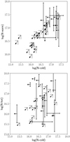 |
Fig. 3 Best-fit column densities for the cold (Ar I), warm (Ar II+Ar III), and hot (Ar XVI+Ar XVII+Ar XVIII) ISM phases. |
Best-fit argon column densities obtained.
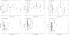 |
Fig. 4 Ar column densities distribution for each ISM phase as a function of Galactic latitude (top panels) and Galactic longitude (bottom panels). Upper values have not been included for illustrative purposes. |
4 The Ar edge
4.1 Best-fit results
Table 3 shows the best-fit results. We have distinguished between different phases of the gaseous ISM, categorizing them as cold (Ar I), warm (Ar II+Ar III), and hot (Ar XVI+Ar XVII+Ar XVIII). These phases were defined following the analysis of the ISM X-ray absorption done by Gatuzz & Churazov (2018), in which the cold component includes the neutral and molecular gas and corresponds to Te < 1 × 10⁴ K, the warm component corresponds to Te ~ 5 × 10⁴ K, and the hot component to Te ~ 1 × 10⁶ K. We note that upper limits were obtained for relevant parameters for most sources. The obtained best-fit column densities are depicted in Fig. 3, indicating column densities within similar ranges across different gaseous phases.
Figure 4 illustrates the distribution of column densities for each phase of the ISM concerning the Galactic latitude (top panels) and Galactic longitude (bottom panels). Despite our efforts, establishing a correlation with Galactic latitude remains challenging, with many sources yielding upper-limit results. This echoes findings by Gatuzz et al. (2021, 2023b), who observe a consistent distribution of the warm-hot ISM component in their analysis of nitrogen and sulfur K-edge photoabsorption regions, alongside a decline in the cold component. Figure 5 presents the column density distribution for each phase relative to the distance for applicable sources. Although there is a hint of a decreasing column density as a function of distance for the cold-warm phases, discerning a clear correlation between these parameters proves elusive.
While this study represents the first in-depth exploration of Argon X-ray absorption using high-resolution spectra, it is pertinent to consider comparisons with previous research. Prior analyses of the ISM utilizing X-ray absorption have revealed a predominance of the neutral component, with mass fractions for various phases in the Galactic disc at approximately ~90% for neutral phases, ~8% for warm ones, and ~2% for hot ones (e.g., Yao & Wang 2006; Pinto et al. 2013; Gatuzz & Churazov 2018). However, due to us predominantly obtaining upper limits in our study, accurate computation of mass fractions for all sources proves challenging. We do not consider ionization equilibrium for argon ionic species, as the column densities in the ISMabs model are treated as free parameters. Therefore, the temperature of the hot phase may not be sufficiently high to yield highly ionized Ar. Furthermore, the hot phase may include contributions from ionized static absorbers intrinsic to the source (see, for example, Gatuzz et al. 2020a). It is commonly assumed that the neutral component of the ISM exponentially decreases in the perpendicular direction to the Galactic plane, with larger column densities observed near the Galactic center (see, e.g., Robin et al. 2003; Kalberla & Kerp 2009; Gatuzz et al. 2024b). Nevertheless, argon depletion into dust may deviate from such distribution patterns, which could impact the observed column densities in both the cold and warm ISM atomic phases. Depending on the level of depletion, the X-ray absorption lines attributable to gas-phase argon would be weaker than expected, potentially leading to an underestimation of the argon abundance and also affecting the benchmarking of the atomic data (Costantini & Corrales 2022). While a comprehensive thermodynamic analysis of the ISM component, incorporating dust depletion effects, is beyond the scope of this study, acknowledging its potential impact on the observed column densities highlights an important area for future research.
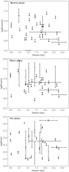 |
Fig. 5 Ar column densities distribution for each ISM phase as a function of the distance. Upper values have not been included for illustrative purposes. |
4.2 Future prospects
Future advancements in X-ray observatories will allow us to resolve the intricate Kα resonance lines across various argon ionic species. An illustration of this potential is depicted in Fig. 6 (top panel), showing a simulation focused on a Galactic source, specifically 4U 1916-053, achieved through Athena (Nandra et al. 2013). This simulation, done with the sixte software (Dauser et al. 2019), integrates the response files of the Athena X-ray Integral Unit (X-IFU), distributed after the reformulation of the Athena mission (Barret et al. 2023). In particular, we adopted an instrumental spectral resolution of 3 eV and a nominal X-IFU configuration without a filter. We also simulated a 250 ks XRISM observation using the same model in combination with the response files available for the XRISM Guest Observer Cycle 1 program (Fig. 6, bottom panel). The XRISM observatory was launched successfully on September 7, releasing its first light on January 5 and showing unprecedented high-resolution spectra for the Perseus cluster and the supernova remnant N132D, becoming the current X-ray community observatory.
The plot shows the remarkable capabilities of the instrument, where prominent resonance absorption lines emerge distinctly, facilitating comprehensive investigations into the multiphase ISM. Furthermore, the simultaneous measurement of Kα and Kβ absorption lines for identical ions promises more accurate constraints on abundances, broadening effects, and ionization state estimation. We note that this simulation exclusively accounts for the gaseous component of the ISM. Although the cumulative dust contribution could be quantified, distinguishing between various dust samples poses a more intricate challenge. For a comprehensive understanding, Costantini et al. (2019) conducted an exhaustive dust simulation tailored for Athena.
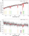 |
Fig. 6 Athena X-IFU (top panel) and XRISM (bottom panel) simulations of the Ar K-edge photoabsorption region for a Galactic source (e.g., 4U 1916-053). The total exposure time is indicated. |
5 Conclusions
We have analyzed the argon K-edge X-ray absorption region (3.1–4.2 Å) using Chandra high-resolution spectra of 33 LMXBs. Each source was fit with a simple powerlaw for the continuum and a modified version of the ISMabs model. Our study provides detailed calculations of new photoabsorption cross sections for Ar I, Ar II, and Ar XVI. Using this model, we derived column density estimates for Ar I, Ar II, Ar III, Ar XVI, Ar XVII, and Ar XVIII ionic species Our analysis revealed that individual Kα doublets/triplets could not be resolved, leading to upper limits for most sources. Furthermore, we observed no correlation between Galactic longitude and latitude, although there were indications of decreasing column density with distance. Finally, our results from the Athena X-IFU and XRISM simulations demonstrate that these observatories will enable unprecedented precision in atomic data benchmarking. Their high-resolution capabilities will allow us to resolve intricate spectral features that were previously inaccessible, leading to more accurate atomic models and a deeper understanding of the physical conditions in various astrophysical environments.
Data availability
Observations analyzed in this article are available in the Chandra Grating-Data Archive and Catalog (TGCat) (http://tgcat.mit.edu/about.php). The ISMabs model is included in the XSPEC data analysis software (https://heasarc.gsfc.nasa.gov/xanadu/xspec/). This research was carried out on the High Performance Computing resources of the cobra cluster at the Max Planck Comput-ing and Data Facility (MPCDF) in Garching operated by the Max Planck Society (MPG).
Appendix A Chandra observation IDs
Table A.1 lists the Chandra observation IDs analyzed in this work.
IDs of the Chandra observations analyzed.
References
- Amayo, A., Delgado-Inglada, G., & Stasińska, G. 2021, MNRAS, 505, 2361 [CrossRef] [Google Scholar]
- Arendt, R. G., Dwek, E., Kober, G., Rho, J., & Hwang, U. 2014, ApJ, 786, 55 [NASA ADS] [CrossRef] [Google Scholar]
- Bandyopadhyay, R. M., Shahbaz, T., Charles, P. A., & Naylor, T. 1999, MNRAS, 306, 417 [Google Scholar]
- Barret, D., Albouys, V., Herder, J.-W. D., et al. 2023, Exp. Astron., 55, 373 [NASA ADS] [CrossRef] [Google Scholar]
- Baumgardt, H., & Hilker, M. 2018, MNRAS, 478, 1520 [Google Scholar]
- Berrington, K. A., Eissner, W. B., & Norrington, P. H. 1995, Comput. Phys. Commun., 92, 290 [NASA ADS] [CrossRef] [Google Scholar]
- Bhattacharyya, S., Strohmayer, T. E., Markwardt, C. B., & Swank, J. H. 2006, ApJ, 639, L31 [NASA ADS] [CrossRef] [Google Scholar]
- Bigiel, F., Leroy, A., Walter, F., et al. 2008, AJ, 136, 2846 [NASA ADS] [CrossRef] [Google Scholar]
- Burke, P. G. 2011, R-matrix Theory of Atomic Collisions (New York: Springer) [CrossRef] [Google Scholar]
- Churazov, E., Gilfanov, M., Forman, W., & Jones, C. 1996, ApJ, 471, 673 [NASA ADS] [CrossRef] [Google Scholar]
- Corbel, S., Kaaret, P., Fender, R. P., et al. 2005, ApJ, 632, 504 [CrossRef] [Google Scholar]
- Corrales, L., Gotthelf, E., Gatuzz, E., et al. 2024, AAS/High Energy Astrophys, Div., 21, 104.13 [Google Scholar]
- Costantini, E., & Corrales, L. 2022, in Handbook of X-ray and Gamma-ray Astrophysics (Berlin: Springer Nature), 40 [Google Scholar]
- Costantini, E., Pinto, C., Kaastra, J. S., et al. 2012, A&A, 539, A32 [NASA ADS] [CrossRef] [EDP Sciences] [Google Scholar]
- Costantini, E., Zeegers, S. T., Rogantini, D., et al. 2019, A&A, 629, A78 [NASA ADS] [CrossRef] [EDP Sciences] [Google Scholar]
- Dauser, T., Falkner, S., Lorenz, M., et al. 2019, A&A, 630, A66 [NASA ADS] [CrossRef] [EDP Sciences] [Google Scholar]
- Dopita, M. A., Vogt, F. P. A., Sutherland, R. S., et al. 2018, ApJS, 237, 10 [NASA ADS] [CrossRef] [Google Scholar]
- Dopita, M. A., Seitenzahl, I. R., Sutherland, R. S., et al. 2019, AJ, 157, 50 [Google Scholar]
- Draine, B. T. 2011, Physics of the Interstellar and Intergalactic Medium (Princeton: Princeton University Press) [Google Scholar]
- Falgarone, E., Verstraete, L., Pineau Des Forêts, G., & Hily-Blant, P. 2005, A&A, 433, 997 [NASA ADS] [CrossRef] [EDP Sciences] [Google Scholar]
- Gaia Collaboration 2020, VizieR Online Data Catalog: I/350 [Google Scholar]
- Galloway, D. K., Psaltis, D., Muno, M. P., & Chakrabarty, D. 2006, ApJ, 639, 1033 [NASA ADS] [CrossRef] [Google Scholar]
- Gatuzz, E., & Churazov, E. 2018, MNRAS, 474, 696 [NASA ADS] [CrossRef] [Google Scholar]
- Gatuzz, E., García, J., Mendoza, C., et al. 2013a, ApJ, 778, 83 [CrossRef] [Google Scholar]
- Gatuzz, E., García, J., Mendoza, C., et al. 2013b, ApJ, 768, 60 [NASA ADS] [CrossRef] [Google Scholar]
- Gatuzz, E., García, J., Mendoza, C., et al. 2014, ApJ, 790, 131 [NASA ADS] [CrossRef] [Google Scholar]
- Gatuzz, E., García, J., Kallman, T. R., Mendoza, C., & Gorczyca, T. W. 2015, ApJ, 800, 29 [NASA ADS] [CrossRef] [Google Scholar]
- Gatuzz, E., García, J. A., Kallman, T. R., & Mendoza, C. 2016, A&A, 588, A111 [NASA ADS] [CrossRef] [EDP Sciences] [Google Scholar]
- Gatuzz, E., Ness, J. U., Gorczyca, T. W., et al. 2018a, MNRAS, 479, 2457 [NASA ADS] [CrossRef] [Google Scholar]
- Gatuzz, E., Rezaei, K. S., Kallman, T. R., et al. 2018b, MNRAS, 479, 3715 [CrossRef] [Google Scholar]
- Gatuzz, E., García, J. A., & Kallman, T. R. 2019, MNRAS, 483, L75 [NASA ADS] [CrossRef] [Google Scholar]
- Gatuzz, E., Díaz Trigo, M., Miller-Jones, J. C. A., & Migliari, S. 2020a, MNRAS, 491, 4857 [CrossRef] [Google Scholar]
- Gatuzz, E., Gorczyca, T. W., Hasoglu, M. F., et al. 2020b, MNRAS, 498, L20 [NASA ADS] [CrossRef] [Google Scholar]
- Gatuzz, E., García, J. A., & Kallman, T. R. 2021, MNRAS, 504, 4460 [NASA ADS] [CrossRef] [Google Scholar]
- Gatuzz, E., García, J. A., Churazov, E., & Kallman, T. R. 2023a, MNRAS, 521, 3098 [NASA ADS] [CrossRef] [Google Scholar]
- Gatuzz, E., Gorczyca, T. W., Hasoglu, M. F., et al. 2023b, MNRAS, 527, 1648 [Google Scholar]
- Gatuzz, E., Wilms, J., Zainab, A., et al. 2024b, A&A, 688, A207 [NASA ADS] [CrossRef] [EDP Sciences] [Google Scholar]
- Gorczyca, T. W. 2000, Phys. Rev. A, 61, 024702 [CrossRef] [Google Scholar]
- Gorczyca, T. W., & Robicheaux, F. 1999, Phys. Rev. A, 60, 1216 [CrossRef] [Google Scholar]
- Gorczyca, T. W., Robicheaux, F., Pindzola, M. S., Griffin, D. C., & Badnell, N. R. 1995, Phys. Rev. A, 52, 3877 [NASA ADS] [CrossRef] [Google Scholar]
- Gorczyca, T. W., & McLaughlin, B. M. 2000, J. Phys. B Atm. Mol. Phys., 33, L859 [NASA ADS] [CrossRef] [Google Scholar]
- Gorczyca, T. W., Bautista, M. A., Hasoglu, M. F., et al. 2013, ApJ, 779, 78 [CrossRef] [Google Scholar]
- Grimm, H.-J., Gilfanov, M., & Sunyaev, R. 2002, A&A, 391, 923 [NASA ADS] [CrossRef] [EDP Sciences] [Google Scholar]
- Hasoglu, M. F., Abdel-Naby, S. A., Gorczyca, T. W., Drake, J. J., & McLaughlin, B. M. 2010, ApJ, 724, 1296 [CrossRef] [Google Scholar]
- Hasoğlu, M. F., Abdel-Naby, S. A., Gatuzz, E., et al. 2014, ApJS, 214, 8 [CrossRef] [Google Scholar]
- Hua, Z., Li, Z., Zhang, M., Chen, Z., & Morris, M. R. 2023, MNRAS, 522, 635 [NASA ADS] [CrossRef] [Google Scholar]
- Hynes, R. I., Steeghs, D., Casares, J., Charles, P. A., & O’Brien, K. 2004, ApJ, 609, 317 [Google Scholar]
- Iaria, R., di Salvo, T., Robba, N. R., et al. 2005, A&A, 439, 575 [NASA ADS] [CrossRef] [EDP Sciences] [Google Scholar]
- in‘t Zand, J. J. M., Kuulkers, E., Verbunt, F., Heise, J., & Cornelisse, R. 2003, A&A, 411, L487 [CrossRef] [EDP Sciences] [Google Scholar]
- Jenkins, E. B., & Tripp, T. M. 2011, ApJ, 734, 65 [NASA ADS] [CrossRef] [Google Scholar]
- Joachimi, K., Gatuzz, E., García, J. A., & Kallman, T. R. 2016, MNRAS, 461, 352 [NASA ADS] [CrossRef] [Google Scholar]
- Jones, O. C., Kavanagh, P. J., Barlow, M. J., et al. 2023, ApJ, 958, 95 [CrossRef] [Google Scholar]
- Jonker, P. G., & Nelemans, G. 2004, MNRAS, 354, 355 [Google Scholar]
- Kalberla, P. M., & Kerp, J. 2009, ARA&A, 47, 27 [NASA ADS] [CrossRef] [Google Scholar]
- Kobayashi, C., Karakas, A. I., & Lugaro, M. 2020, ApJ, 900, 179 [Google Scholar]
- Kong, A. K. H., Homer, L., Kuulkers, E., Charles, P. A., & Smale, A. P. 2000, MNRAS, 311, 405 [NASA ADS] [CrossRef] [Google Scholar]
- Kramida, A. E., Ralchenko, Y., Reader, J., & NIST ASD Team 2020, National Institute of Standards and Technology, http://physics.nist.gov/asd [Google Scholar]
- Lada, C. J., Lombardi, M., & Alves, J. F. 2010, ApJ, 724, 687 [Google Scholar]
- Leroy, A. K., Walter, F., Brinks, E., et al. 2008, AJ, 136, 2782 [Google Scholar]
- Leung, S.-C., & Nomoto, K. 2018, ApJ, 861, 143 [Google Scholar]
- Lilly, S. J., Carollo, C. M., Pipino, A., Renzini, A., & Peng, Y. 2013, ApJ, 772, 119 [NASA ADS] [CrossRef] [Google Scholar]
- López-Sánchez, Á. R., & Esteban, C. 2010, A&A, 517, A85 [NASA ADS] [CrossRef] [EDP Sciences] [Google Scholar]
- Mason, K. O., & Cordova, F. A. 1982, ApJ, 262, 253 [NASA ADS] [CrossRef] [Google Scholar]
- McKee, C. F., & Ostriker, J. P. 1977, ApJ, 218, 148 [NASA ADS] [CrossRef] [Google Scholar]
- Nandra, K., Barret, D., Barcons, X., et al. 2013, arXiv e-prints [arXiv:1306.2307] [Google Scholar]
- Ogliore, R. C., Stone, E. C., Leske, R. A., et al. 2009, ApJ, 695, 666 [CrossRef] [Google Scholar]
- Oosterbroek, T., Barret, D., Guainazzi, M., & Ford, E. C. 2001, A&A, 366, 138 [NASA ADS] [CrossRef] [EDP Sciences] [Google Scholar]
- Paerels, F., Brinkman, A. C., van der Meer, R. L. J., et al. 2001, ApJ, 546, 338 [NASA ADS] [CrossRef] [Google Scholar]
- Palla, M. 2021, MNRAS, 503, 3216 [Google Scholar]
- Pinto, C., Kaastra, J. S., Costantini, E., & Verbunt, F. 2010, A&A, 521, A79 [NASA ADS] [CrossRef] [EDP Sciences] [Google Scholar]
- Pinto, C., Kaastra, J. S., Costantini, E., & de Vries, C. 2013, A&A, 551, A25 [NASA ADS] [CrossRef] [EDP Sciences] [Google Scholar]
- Psaradaki, I., Costantini, E., Mehdipour, M., et al. 2020, A&A, 642, A208 [NASA ADS] [CrossRef] [EDP Sciences] [Google Scholar]
- Psaradaki, I., Costantini, E., Rogantini, D., et al. 2023, A&A, 670, A30 [NASA ADS] [CrossRef] [EDP Sciences] [Google Scholar]
- Psaradaki, I., Corrales, L., Werk, J., et al. 2024, AJ, 167, 217 [NASA ADS] [CrossRef] [Google Scholar]
- Robin, A. C., Reylé, C., Derrière, S., & Picaud, S. 2003, A&A, 409, 523 [NASA ADS] [CrossRef] [EDP Sciences] [Google Scholar]
- Rogantini, D., Costantini, E., Zeegers, S. T., et al. 2018, A&A, 609, A22 [NASA ADS] [CrossRef] [EDP Sciences] [Google Scholar]
- Rogantini, D., Costantini, E., Mehdipour, M., et al. 2021, A&A, 645, A98 [NASA ADS] [CrossRef] [EDP Sciences] [Google Scholar]
- Rupke, D. S. N., & Veilleux, S. 2013, ApJ, 768, 75 [Google Scholar]
- Seitenzahl, I. R., Ciaraldi-Schoolmann, F., Röpke, F. K., et al. 2013, MNRAS, 429, 1156 [NASA ADS] [CrossRef] [Google Scholar]
- Smith, F. T. 1960, Phys. Rev., 118, 349 [NASA ADS] [CrossRef] [Google Scholar]
- Stanimirović, S., & Zweibel, E. G. 2018, ARA&A, 56, 489 [Google Scholar]
- Strom, A. L., Rudie, G. C., Trainor, R. F., et al. 2023, ApJ, 958, L11 [NASA ADS] [CrossRef] [Google Scholar]
- Tonnesen, S., & Bryan, G. L. 2009, ApJ, 694, 789 [NASA ADS] [CrossRef] [Google Scholar]
- Verner, D. A., Ferland, G. J., Korista, K. T., & Yakovlev, D. G. 1996, ApJ, 465, 487 [Google Scholar]
- Wang, Z., & Chakrabarty, D. 2004, ApJ, 616, L139 [NASA ADS] [CrossRef] [Google Scholar]
- Westphal, A. J., Butterworth, A. L., Tomsick, J. A., & Gainsforth, Z. 2019, ApJ, 872, 66 [NASA ADS] [CrossRef] [Google Scholar]
- Willingale, R., Starling, R. L. C., Beardmore, A. P., Tanvir, N. R., & O’Brien, P. T. 2013, MNRAS, 431, 394 [Google Scholar]
- Witthoeft, M. C., García, J., Kallman, T. R., et al. 2011, ApJS, 192, 7 [NASA ADS] [CrossRef] [Google Scholar]
- Wong, T., & Blitz, L. 2002, ApJ, 569, 157 [CrossRef] [Google Scholar]
- Yang, J., Schulz, N. S., Rogantini, D., et al. 2022, AJ, 164, 182 [NASA ADS] [CrossRef] [Google Scholar]
- Yao, Y., & Wang, Q. D. 2006, ApJ, 641, 930 [CrossRef] [Google Scholar]
- Zeegers, S. T., Costantini, E., Rogantini, D., et al. 2019, A&A, 627, A16 [NASA ADS] [CrossRef] [EDP Sciences] [Google Scholar]
- Zhukovska, S., Dobbs, C., Jenkins, E. B., & Klessen, R. S. 2016, ApJ, 831, 147 [NASA ADS] [CrossRef] [Google Scholar]
All Tables
All Figures
|
Fig. 1 Photoabsorption cross sections included in the model for Ar I (top panel), Ar II, Ar III (middle panel), Ar XVI, Ar XVII, and Ar XVIII (bottom panel). The plots also include an Ar I cross section from Verner et al. (1996) and Ar II, Ar III, and Ar XVI cross sections from Witthoeft et al. (2011). |
| In the text | |
|
Fig. 2 Best-fit results in the Ar K-edge photoabsorption region for the LMXB 4U 1916-053. Black points correspond to the observation in flux units, while the red line corresponds to the best-fit model. Residuals are included in units of (data − model)/error. The position of the Kα absorption lines are indicated for each ion, following the color code used in Fig. 1. |
| In the text | |
|
Fig. 3 Best-fit column densities for the cold (Ar I), warm (Ar II+Ar III), and hot (Ar XVI+Ar XVII+Ar XVIII) ISM phases. |
| In the text | |
|
Fig. 4 Ar column densities distribution for each ISM phase as a function of Galactic latitude (top panels) and Galactic longitude (bottom panels). Upper values have not been included for illustrative purposes. |
| In the text | |
|
Fig. 5 Ar column densities distribution for each ISM phase as a function of the distance. Upper values have not been included for illustrative purposes. |
| In the text | |
|
Fig. 6 Athena X-IFU (top panel) and XRISM (bottom panel) simulations of the Ar K-edge photoabsorption region for a Galactic source (e.g., 4U 1916-053). The total exposure time is indicated. |
| In the text | |
Current usage metrics show cumulative count of Article Views (full-text article views including HTML views, PDF and ePub downloads, according to the available data) and Abstracts Views on Vision4Press platform.
Data correspond to usage on the plateform after 2015. The current usage metrics is available 48-96 hours after online publication and is updated daily on week days.
Initial download of the metrics may take a while.