| Issue |
A&A
Volume 687, July 2024
|
|
|---|---|---|
| Article Number | A294 | |
| Number of page(s) | 7 | |
| Section | Stellar structure and evolution | |
| DOI | https://doi.org/10.1051/0004-6361/202450341 | |
| Published online | 23 July 2024 | |
Constraining the helium-to-metal enrichment ratio ΔY/ΔZ from main-sequence binary stars
Theoretical analysis of the accuracy and precision of the age and helium abundance estimates
1
Dipartimento di Fisica “Enrico Fermi”, Università di Pisa, Largo Pontecorvo 3, 56127 Pisa, Italy
e-mail: valle@df.unipi.it
2
INFN, Sezione di Pisa, Largo Pontecorvo 3, 56127 Pisa, Italy
Received:
12
April
2024
Accepted:
13
May
2024
Aims. We aim to investigate the theoretical possibility of accurately determining the helium-to-metal enrichment ratio ΔY/ΔZ from precise observations of double-lined eclipsing binary systems.
Methods. Using Monte Carlo simulations, we drew synthetic binary systems with masses between 0.85 and 1.00 M⊙ from a grid of stellar models. Both stars were sampled from a grid with ΔY/ΔZ = 2.0, with a primary star at 80% of its main-sequence evolution. Subsequently, a broader grid with ΔY/ΔZ from 1.0 to 3.0 was used in the fitting process. To account for observational uncertainties, two scenarios were explored: S1, with realistic uncertainties of 100 K in temperature and 0.1 dex in [Fe/H]; and S2, with halved uncertainties. We repeated the simulation at two baseline metallicities: [Fe/H] = 0.0 and −0.3.
Results. The posterior distributions of ΔY/ΔZ revealed significant biases. The distributions were severely biased towards the edge of the allowable range in the S1 error scenario. The situation only marginally improved when considering the S2 scenario. The effect is due to the impact of changing ΔY/ΔZ in the stellar effective temperature and its interplay with [Fe/H] observational error, and it is therefore not restricted to the specific fitting method. Despite the presence of these systematic discrepancies, the age of the systems were recovered unbiased with 10% precision.
Conclusions. Our findings indicate that the observational uncertainty in effective temperature and metallicity significantly hinders the accurate determination of the ΔY/ΔZ parameter from main-sequence binary systems.
Key words: methods: statistical / binaries: eclipsing / stars: evolution / stars: fundamental parameters / stars: interiors
© The Authors 2024
 Open Access article, published by EDP Sciences, under the terms of the Creative Commons Attribution License (https://creativecommons.org/licenses/by/4.0), which permits unrestricted use, distribution, and reproduction in any medium, provided the original work is properly cited.
This article is published in open access under the Subscribe to Open model. Subscribe to A&A to support open access publication.
1. Introduction
While stellar model predictions have significantly improved in recent decades, they still face shortcomings in their modelling of certain physical phenomena such as convective transport (see Viallet et al. 2015 for an introduction) or the effects of microscopic diffusion and of the mechanisms competing with it (see e.g. Moedas et al. 2022). In this context, binary systems are often adopted to calibrate free parameters in stellar model computations. This is particularly true following the improvement in the radius and mass precision for stars in a binary system (thanks to satellite missions such as Kepler and TESS Borucki et al. 2010; Ricker et al. 2015), alongside progressions in the methods of estimating the stellar effective temperatures (Miller et al. 2020). Nowadays, a level of precision in the measured parameters below 1% is not uncommon, and several binary systems have masses and radii measured with 0.1% levels of precision.
In addition to their sensitivity to the underlying physics, stellar models are also influenced by the assumed chemical composition, particularly the abundance of helium (Y), and the total metallicity (Z). While surface metallicity can be measured from absorption lines of several metals in the stellar spectra, determining the helium abundance for the majority of stars is not possible due to the absence of observable helium lines in stars cooler than approximately 20 000 K. From a theoretical perspective, this necessitates the assumption of an initial helium abundance for stellar evolution computations. The conventional approach involves adopting a linear relationship between the helium abundance and metallicity,  , where Yp is the primordial helium abundance produced in the Big Bang nucleosynthesis and ΔY/ΔZ is the helium-to-metal enrichment ratio.
The determination of the value of ΔY/ΔZ has received significant attention in the literature. Several methods have been employed to constrain its value, including comparing isochrones and observations in the HR diagram (e.g. Pagel & Portinari 1998; Casagrande et al. 2007; Gennaro et al. 2010; Tognelli et al. 2021); fitting stellar tracks on a survey of nearby field stars (Valcarce et al. 2013); constructing a standard solar model that reproduces the Sun’s present luminosity, radius, and surface Z/X ratio (e.g Gennaro et al. 2010; Serenelli 2010; Tognelli et al. 2011; Valcarce et al. 2012); and calibrating models with evolved stars (horizontal branch and red giant stars, Renzini 1994; Marino et al.2014; Valcarce et al. 2016) using galactic and extragalactic H II regions (e.g. Peimbert & Torres-Peimbert 1974; Pagel et al. 1992; Chiappini & Maciel 1994; Peimbert et al. 2000; Fukugita & Kawasaki 2006; Méndez-Delgado et al. 2020) or planetary nebula (D’Odorico et al. 1976; Chiappini & Maciel 1994; Peimbert & Serrano 1980; Maciel 2001). The results from these diverse approaches exhibit large variability and potential systematic uncertainties. For instance, standard solar models suggest ΔY/ΔZ ≲ 1, whereas evolved stars favour ΔY/ΔZ ∈ [2, 3], and HR diagram comparisons typically indicate values within the [1, 3] range.
Another possibility to constrain the helium-to-metal enrichment ratio comes from detached, double-lined eclipsing binaries (EBs). These systems offer the opportunity to precisely determine the masses, radii, and effective temperatures of their stellar components. Since these stars are presumed to share a common age and initial chemical composition, they serve as an ideal experimental environment for stellar-evolution-model calibration. By comparing these models to observed properties of EBs, it is possible to gain deeper insights into fundamental stellar processes, such as the treatment of convection and diffusion (see, among others, Andersen et al. 1991; Torres et al. 2010; Nataf et al. 2012; Valle et al. 2017, 2023a; Claret & Torres 2017). Early investigations (Ribas et al. 2000; Fernandes et al. 2012) suggested a value of ΔY/ΔZ = 2 ± 1, with some systems exhibiting higher values. However, the primordial helium abundance inferred from these studies was Yp = 0.225, which is significantly lower than the primordial abundance estimated from Big Bang nucleosynthesis. The increasing precision in mass and radius measurements from binary systems, nowadays often reaching a 0.1% accuracy level, suggests an unprecedented opportunity to further refine the estimation of ΔY/ΔZ.
In this paper, we theoretically explore this possibility through the creation of artificial stars generated from a grid of computed stellar models. By quantifying the statistical and systematic uncertainties affecting the ΔY/ΔZ estimates in a fully controlled environment, we established the highest achievable precision from EBs. The investigated systems were carefully selected due to the complexity of estimating the helium-to-metal enrichment ratio. This estimation involves simultaneously fitting additional stellar model parameters, such as age, convective-core overshooting efficiency, and mixing-length value (see e.g. Feiden 2015). These parameters significantly impact stellar model calculations of solar-like stars, introducing degeneracies in the fit. Therefore, attempts to fit the ΔY/ΔZ value from observations should rely on carefully chosen EBs. For instance, limiting the analysis to main-sequence (MS) stars without convective cores allows for the neglect of the convective-core overshooting efficiency, effectively eliminating a nuisance parameter.
The structure of the paper is as follows. In Sect. 2, we discuss the grid, the sampling scheme, and the fitting method used in the estimation process. The results are presented in Sect. 3, with an analysis of the metallicity effect. Some concluding remarks can be found in Sect. 4.
2. Methods
2.1. Stellar model grid
The grid of stellar evolutionary models was calculated for the 0.85 to 1.00 M⊙ mass range, spanning the evolutionary stages from the pre-main sequence to the onset of the red giant branch (RGB). The initial metallicity [Fe/H] was varied from −0.5 dex to 0.2 dex with a step of 0.01 dex. We adopted the solar heavy-element mixture by Asplund et al. (2009). For each metallicity, we considered a range of initial helium abundances based on the commonly used linear relation  with the primordial helium abundance Yp = 0.2471 from Planck Collaboration VI (2020). The helium-to-metal enrichment ratio ΔY/ΔZ was varied from 1.0 to 3.0 with a step of 0.1.
Models were computed with the FRANEC code, in the same configuration as was adopted to compute the Pisa Stellar Evolution Data Base1 for low-mass stars (Dell’Omodarme et al. 2012). The only difference with respect to those models is that in the present research the outer boundary conditions were set by the solar semi-empirical T(τ), of Vernazza et al. (1981), which approximate results obtained using the hydro-calibrated T(τ) well (Salaris & Cassisi 2015; Salaris et al. 2018). The models were computed assuming the solar-scaled mixing-length parameter αml = 2.02. Atomic diffusion was included adopting the coefficients given by Thoul et al. (1994) for gravitational settling and thermal diffusion. To prevent extreme variations in the surface chemical abundances, the diffusion velocities were multiplied by a suppression parabolic factor that takes a value of one for 99% of the mass of the structure and zero at the base of the atmosphere (Chaboyer et al. 2001).
Raw stellar evolutionary tracks were reduced to a set of tracks with the same number of homologous points according to the evolutionary phase. Details about the reduction procedure are reported in the appendix of Valle et al. (2013). Given the accuracy in the observational radius data, a linear interpolation in time was performed for every reduced track. This was done to ensure that the separation in radius between consecutive track points in the 10σ range from the observational targets was less than a quarter of the adopted radius uncertainty.
2.2. Sampling scheme
Artificial binary systems were constructed as follows. Primary stars were selected from the grid of models with mass values in the set of Mp = 0.85, 0.90, 0.95, 1.00 M⊙; metallicities of [Fe/H] = 0.0 and −0.3; and ΔY/ΔZ = 2.0. The stars were selected when they reached 80% of their MS lifetime, as this is when the effect of the helium abundance difference is most pronounced (Valle et al. 2015a). The lower mass boundary was chosen in a way that every star could reach the evolutionary sampling point within the age of the Universe. The higher boundary was determined such that convective-core overshooting could be safely disregarded, because stars in the chosen mass range burn hydrogen in a radiative core. Each primary star was paired with a secondary within the same mass set that was limited to the primary’s mass value and had the same chemical composition and age as the primary star. This selection yielded ten systems for each [Fe/H] value.
The observational constraints taken into account were effective temperature (Teff), metallicity [Fe/H], mass, and radius. We also tested a different scenario adopting stellar log luminosity instead of effective temperature as the observational constraint, obtaining a noticeable agreement in the results. We therefore focus only on the former scenario. Two sets of observational errors were considered: the first set (S1) represents a realistically achievable precision of 100 K in Teff, 0.1 dex in [Fe/H], and 0.5% in radius and mass. While it is not uncommon to find studies in the literature reporting an accuracy of a few tenths of a kelvin in Teff, direct comparisons of results obtained by different authors for the same stars often reveal discrepancies exceeding 100 K (see e.g. Ramírez & Meléndez 2005; Schmidt et al. 2016). The second set (S2) assumes over-optimistically precise measurements of 50 K in Teff, 0.05 dex in [Fe/H] (see e.g. Yu et al. 2023; Hegedüs et al. 2023), and 0.5% in radius and mass.
The selected system observables were subjected to random Gaussian perturbations to simulate observation uncertainties while taking into account the correlation structure among the observational data for the two stars. Following Valle et al. (2017, 2023a), we assumed a correlation of 0.95 between the primary and secondary effective temperatures and 0.95 between the metallicities of the two stars. Regarding mass and radius correlations, the high precision level of the estimates means that these parameters are of no importance. For each binary system, N = 5 000 perturbed systems were generated.
Each perturbed system underwent parameter estimation (as explained in Sect. 2.3), assuming identical chemical composition and age for both the primary and secondary stars. Only solutions providing a satisfactory fit (determined by their χ2 values) were retained in the final sample. From these samples, marginalised posterior distributions of the age and helium-to-metal enrichment ratio were obtained.
2.3. Fitting technique
The analysis is conducted adopting the SCEPtER pipeline2, a well-tested technique for fitting single and binary systems (e.g. Valle et al. 2014, 2015b,a; Valle et al. 2017, 2023b). The pipeline estimates the parameters of interest (i.e. the system age and its initial chemical abundances), adopting a grid maximum-likelihood approach.
The method we used is explained in detail in Valle et al. (2015a); here, we provide only a brief summary for convenience. For every jth point in the fitting grid of precomputed stellar models, a likelihood estimate is obtained for both stars:
where oi are the n observational constraints,  are the jth grid point corresponding values, and σi are the observational uncertainties.
The joint likelihood of the system is then computed as the product of the single star likelihood functions. Information about effective temperature and mass ratios was adopted as multiplicative Gaussian priors. However, we directly verified that their impact in the results was negligible, because the correlations in the Monte Carlo samples (Sect. 2.2) translate to correlations between the fitted parameters (see Appendix A). It is possible to obtain estimates both for the individual components and for the whole system. In the former case, the fits for the two stars are obtained independently, while in the latter case the two objects must have a common age (with a tolerance of 1 Myr), identical initial helium abundance, and identical initial metallicity. Stellar parameter estimates were obtained by averaging the corresponding quantity of all the models with a likelihood greater than  3.
3.
3. Results
3.1. Artificial stars with [Fe/H] = 0.0
The Monte Carlo simulations reveal that the estimation of the ΔY/ΔZ parameter is extremely challenging in all examined scenarios. The left panel of Fig. 1 shows the posterior distributions of the helium-to-metal enrichment ratio for the studied binary systems assuming S1 uncertainties. All distributions display a similar pattern, with two peaks located at the edges of the explored range rather than close to the true value of ΔY/ΔZ = 2.0. The situation slightly improves when considering the S2 lower observational uncertainties (right panel in Fig. 1), because some systems show a posterior mildly peaked around the true value. However, all the posterior distributions have a large variance, and the ΔY/ΔZ parameter is effectively unconstrained across the entire range. Therefore, even in this overly optimistic scenario in which artificial stars and models perfectly align, save for random uncertainties, binary systems fail to provide a reliable estimate of the helium-to-metal enrichment ratio. The estimation is even more problematic when attempted using real-world binary systems, as systematic discrepancies between models and stars are expected.
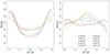 |
Fig. 1. Kernel density estimators of helium-to-metal enrichment ratio for different binary systems. Left: density estimates obtained employing error set S1. Right: same as in the left panel, but adopting error set S2. |
The presence of peaks at the edges of the considered range is not surprising, as has been reported in previous works using both artificial and real binary systems (Valle et al. 2017, 2018, 2023a). The underlying cause of these peaks and the differences between the two panels in Fig. 1 lies in the interplay between helium entrenchment and the effect of the [Fe/H] on the effective temperature. The two panels of Fig. 2 show the stellar evolutionary tracks for a 0.85 M⊙ star (left panel) and 1.00 M⊙ star (right panel), both with [Fe/H] = 0.0 and ΔY/ΔZ = 2.0, alongside other tracks for the same masses; however, this is with [Fe/H] = 0.1 and a varying ΔY/ΔZ. A metallicity error of 0.1 dex, equivalent to the assumed observational uncertainty in the S1 scenario, displaces the stellar track of a 0.85 M⊙ model in effective temperature from 5578 K to 5478 K. This difference cannot be compensated even by the most helium-rich model, because its effective temperature at the radius constraint is only 5564 K. Consequently, in this scenario the likelihood algorithm only considers models with ΔY/ΔZ = 3.0 in the fit. A similar pattern is observed for 1.00 M⊙ models. The opposite scenario arises when [Fe/H] is underestimated, leading to an over-representation of solutions with ΔY/ΔZ = 1.0. Only when the perturbations in [Fe/H] and Teff counteract each other are solutions within the middle of the range explored. The presence of the two significant peaks at the edge of the range is therefore an artefact. If a broader range of ΔY/ΔZ is allowed during the fitting process, the height of the peaks in the posterior distributions diminish, and the distributions tend to become nearly uniform, as observed for several systems in the right panel of the figure.
 |
Fig. 2. Stellar tracks for different masses, [Fe/H], and ΔY/ΔZ. Left: evolutionary tracks for M = 0.85 M⊙. The solid line corresponds to [Fe/H] = 0.0, and ΔY/ΔZ = 2.0. Dashed lines correspond to [Fe/H] = 0.1 for different values of ΔY/ΔZ. The dotted line marks the radius value at 80% of the evolution in MS. Right: same as in left panel, but for M = 1.00 M⊙. |
The difficulty in accurately determining the ΔY/ΔZ value has a limited influence on the estimation of the systems age. Figure 3 shows that the relative error in the age remains centred around zero, even under scenario S1. Table 1 reports the median values of these distributions (q50) and the corresponding 16th and 84th percentiles (q16 and q84, respectively), adopted as the boundary of the 1 σ interval. The average width of these distributions, calculated as the half-width of the interval between q16 and q84, is about 10%. When observational data are more precise, the distributions of the age relative error shrink (right panel of Fig. 3 and last three columns in Table 1). In fact, the average width of these distributions is about 6.5%, that is, three-quarters of the values found in S1 scenario. In the S1 scenario, the marginalised posterior distribution of the relative errors in stellar ages exhibits a multi-modal feature, which arises from the presence of multiple peaks in the estimated helium-to-metal enrichment ratios. This feature is less prominent in the S2 scenario, as evidenced by the right panel of Fig. 3. Several systems in this scenario exhibit a unimodal distribution.
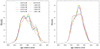 |
Fig. 3. Kernel density estimators of relative error in the estimated age for different binary systems. Left: densities obtained adopting error set S1. Right: same as in left panel, but using error set S2. |
Percentiles of the relative error in the age estimates from different binary systems.
3.2. Artificial stars with [Fe/H] = −0.3
Results from Monte Carlo simulations performed for artificial stars with a baseline metallicity of [Fe/H] = −0.3 are even less encouraging than those discussed in the previous section. This unsurprising finding stems from the fact that the lower the metallicity [Fe/H], the narrower the range ΔY spanned by the models. As a consequence, the range in effective temperature spanned by a set of models at fixed [Fe/H] and varying ΔY/ΔZ shrinks. This is clearly seen from Fig. 4, which shows that the extreme variation in the ΔY/ΔZ parameter can compensate about one half of the Teff offset due to a variation of 0.1 dex in the metallicity [Fe/H]. Consequently, the posterior distributions of ΔY/ΔZ are even more peaked at the edges of the allowed range. Even in the S2 scenario, the estimated helium-to-metal enrichment ratio is significantly distorted at this baseline metallicity, as shown in the right panel of Fig. 5.
4. Conclusions
We investigated the feasibility of accurately determining the helium-to-metal enrichment ratio ΔY/ΔZ from precise observations of binary systems. To this end, we performed a theoretical Monte Carlo investigation. Synthetic systems were sampled from a grid of computed stellar models, and the same grid was utilized in the subsequent fitting process. Observational errors were accounted for by adding to the artificial system’s Gaussian noise. Two distinct scenarios were examined: S1, corresponding to a realistically attainable precision of 100 K in effective temperature and 0.1 dex in surface metallicity [Fe/H]; and S2, in which these uncertainties were halved.
Synthetic binary systems were constructed by pairing primary stars with masses between 0.85 and 1.00 M⊙ with secondary stars in the same mass range. Two baseline metallicities were considered: [Fe/H] = 0.0 and −0.3. The systems were drawn from a reference grid with ΔY/ΔZ = 2.0 at the point when the primary star reaches 80% of its MS evolution. This near turn-off phase is particularly sensitive to the influence of varying helium-to-metal enrichment ratios (Valle et al. 2015a). From each system, N = 5000 perturbed Monte Carlo realisations were generated. These synthetic systems were subjected to fitting procedures to determine their age, metallicity Z, and initial helium abundance Y. The resulting best-fit ΔY/ΔZ were computed.
An examination of the posterior distributions of the helium-to-metal enrichment ratio revealed significant biases in the fitted parameter. The distributions were severely biased towards the edge of the allowable range when employing the S1 error scenario. The situation only marginally improved when considering the S2 scenario. This behaviour arises from the magnitude of the impact of varying ΔY/ΔZ on the effective temperatures of stellar models. The considered metallicity uncertainty of 0.1 dex in the S1 scenario produces a larger shift in effective temperature compared to that caused by the extreme variations in helium-to-metal enrichment ratio. This leads to an over-abundance of edge values in the ΔY/ΔZ posterior distributions. This effect is more pronounced at lower metallicities, as the same variability in ΔY/ΔZ translates to a reduced variation in initial helium abundance Y. Therefore, the results presented in this paper are not dependent on the specific fitting algorithm employed and are generally relevant.
While the mass range and the evolutionary phase were carefully selected to minimise or eliminate certain sources of uncertainty, such as the need to account for convective-core overshooting efficiency, our findings indicate that the random variability in effective temperature and metallicity introduced by observational uncertainties significantly hinders the accurate determination of the ΔY/ΔZ parameter. This result confirms the finding of Valle et al. (2018), who reported a similar pattern in the posterior distributions of the ΔY/ΔZ parameter in their theoretical study of more massive and evolved binary systems. The inability to accurately retrieve the true value of the helium-to-metal enrichment ratio, as discussed above, emerges from a theoretical setting devoid of systematic discrepancies between synthetic systems and the underlying model grid. When employing real-world binary systems for this task, even more substantial biases are anticipated. Ultimately, the adoption of binary systems for ΔY/ΔZ investigation appears to be questionable. Fortunately, while determining the precise value of ΔY/ΔZ can be challenging, this has minimal impact on the system age estimation, which achieved a 10% median precision across all studied configurations.
Publicly available on CRAN: http://CRAN.R-project.org/package=SCEPtER, http://CRAN.R-project.org/package=SCEPtERbinary
Acknowledgments
We thank our anonymous referee for the useful comments and suggestions. G.V., P.G.P.M. and S.D. acknowledge INFN (Iniziativa specifica TAsP) and support from PRIN MIUR2022 Progetto “CHRONOS” (PI: S. Cassisi) finanziato dall’Unione Europea – Next Generation EU.
References
- Andersen, J., Clausen, J. V., Nordstrom, B., Tomkin, J., & Mayor, M. 1991, A&A, 246, 99 [NASA ADS] [Google Scholar]
- Asplund, M., Grevesse, N., Sauval, A. J., & Scott, P. 2009, ARA&A, 47, 481 [NASA ADS] [CrossRef] [Google Scholar]
- Borucki, W. J., Koch, D., Basri, G., et al. 2010, Science, 327, 977 [Google Scholar]
- Casagrande, L., Flynn, C., Portinari, L., Girardi, L., & Jimenez, R. 2007, MNRAS, 382, 1516 [NASA ADS] [CrossRef] [Google Scholar]
- Chaboyer, B., Fenton, W. H., Nelan, J. E., Patnaude, D. J., & Simon, F. E. 2001, ApJ, 562, 521 [NASA ADS] [CrossRef] [Google Scholar]
- Chiappini, C., & Maciel, W. J. 1994, A&A, 288, 921 [NASA ADS] [Google Scholar]
- Claret, A., & Torres, G. 2017, ApJ, 849, 18 [Google Scholar]
- Dell’Omodarme, M., Valle, G., Degl’Innocenti, S., & Prada Moroni, P. G. 2012, A&A, 540, A26 [CrossRef] [EDP Sciences] [Google Scholar]
- D’Odorico, S., Peimbert, M., & Sabbadin, F. 1976, A&A, 47, 341 [Google Scholar]
- Feiden, G. A. 2015, in Living Together: Planets, Host Stars and Binaries, eds. S. M. Rucinski, G. Torres, & M. Zejda, ASP Conf. Ser., 496, 137 [NASA ADS] [Google Scholar]
- Fernandes, J., Vaz, A. I. F., & Vicente, L. N. 2012, MNRAS, 425, 3104 [NASA ADS] [CrossRef] [Google Scholar]
- Fukugita, M., & Kawasaki, M. 2006, ApJ, 646, 691 [NASA ADS] [CrossRef] [Google Scholar]
- Gennaro, M., Prada Moroni, P. G., & Degl’Innocenti, S. 2010, A&A, 518, A13 [NASA ADS] [CrossRef] [EDP Sciences] [Google Scholar]
- Hegedüs, V., Mészáros, S., Jofré, P., et al. 2023, A&A, 670, A107 [NASA ADS] [CrossRef] [EDP Sciences] [Google Scholar]
- Maciel, W. J. 2001, Ap&SS, 277, 545 [NASA ADS] [CrossRef] [Google Scholar]
- Marino, A. F., Milone, A. P., Przybilla, N., et al. 2014, MNRAS, 437, 1609 [NASA ADS] [CrossRef] [Google Scholar]
- Méndez-Delgado, J. E., Esteban, C., García-Rojas, J., Arellano-Córdova, K. Z., & Valerdi, M. 2020, MNRAS, 496, 2726 [CrossRef] [Google Scholar]
- Miller, N. J., Maxted, P. F. L., & Smalley, B. 2020, MNRAS, 497, 2899 [Google Scholar]
- Moedas, N., Deal, M., Bossini, D., & Campilho, B. 2022, A&A, 666, A43 [NASA ADS] [CrossRef] [EDP Sciences] [Google Scholar]
- Nataf, D. M., Gould, A., & Pinsonneault, M. H. 2012, Acta Astron., 62, 33 [NASA ADS] [Google Scholar]
- Pagel, B. E. J., & Portinari, L. 1998, MNRAS, 298, 747 [NASA ADS] [CrossRef] [Google Scholar]
- Pagel, B. E. J., Simonson, E. A., Terlevich, R. J., & Edmunds, M. G. 1992, MNRAS, 255, 325 [CrossRef] [Google Scholar]
- Peimbert, M., & Serrano, A. 1980, Rev. Mex. A&A, 5, 9 [NASA ADS] [Google Scholar]
- Peimbert, M., & Torres-Peimbert, S. 1974, ApJ, 193, 327 [NASA ADS] [CrossRef] [Google Scholar]
- Peimbert, M., Peimbert, A., & Ruiz, M. T. 2000, ApJ, 541, 688 [NASA ADS] [CrossRef] [Google Scholar]
- Planck Collaboration VI. 2020, A&A, 641, A6 [NASA ADS] [CrossRef] [EDP Sciences] [Google Scholar]
- Ramírez, I., & Meléndez, J. 2005, ApJ, 626, 465 [Google Scholar]
- Renzini, A. 1994, A&A, 285, L5 [NASA ADS] [Google Scholar]
- Ribas, I., Jordi, C., & Giménez, Á. 2000, MNRAS, 318, L55 [Google Scholar]
- Ricker, G. R., Winn, J. N., Vanderspek, R., et al. 2015, J. Astron. Telesc. Instrum. Syst., 1, 014003 [Google Scholar]
- Salaris, M., & Cassisi, S. 2015, A&A, 577, A60 [CrossRef] [EDP Sciences] [Google Scholar]
- Salaris, M., Cassisi, S., Schiavon, R. P., & Pietrinferni, A. 2018, A&A, 612, A68 [NASA ADS] [CrossRef] [EDP Sciences] [Google Scholar]
- Schmidt, S. J., Wagoner, E. L., Johnson, J. A., et al. 2016, MNRAS, 460, 2611 [Google Scholar]
- Serenelli, A. M. 2010, Ap&SS, 328, 13 [Google Scholar]
- Thoul, A. A., Bahcall, J. N., & Loeb, A. 1994, ApJ, 421, 828 [Google Scholar]
- Tognelli, E., Prada Moroni, P. G., & Degl’Innocenti, S. 2011, A&A, 533, A109 [NASA ADS] [CrossRef] [EDP Sciences] [Google Scholar]
- Tognelli, E., Dell’Omodarme, M., Valle, G., Prada Moroni, P. G., & Degl’Innocenti, S. 2021, MNRAS, 501, 383 [Google Scholar]
- Torres, G., Andersen, J., & Giménez, A. 2010, A&A Rev., 18, 67 [Google Scholar]
- Valcarce, A. A. R., Catelan, M., & Sweigart, A. V. 2012, A&A, 547, A5 [NASA ADS] [CrossRef] [EDP Sciences] [Google Scholar]
- Valcarce, A. A. R., Catelan, M., & De Medeiros, J. R. 2013, A&A, 553, A62 [NASA ADS] [CrossRef] [EDP Sciences] [Google Scholar]
- Valcarce, A. A. R., Catelan, M., Alonso-García, J., Contreras Ramos, R., & Alves, S. 2016, A&A, 589, A126 [NASA ADS] [CrossRef] [EDP Sciences] [Google Scholar]
- Valle, G., Dell’Omodarme, M., Prada Moroni, P. G., & Degl’Innocenti, S. 2013, A&A, 549, A50 [CrossRef] [EDP Sciences] [Google Scholar]
- Valle, G., Dell’Omodarme, M., Prada Moroni, P. G., & Degl’Innocenti, S. 2014, A&A, 561, A125 [NASA ADS] [CrossRef] [EDP Sciences] [Google Scholar]
- Valle, G., Dell’Omodarme, M., Prada Moroni, P. G., & Degl’Innocenti, S. 2015a, A&A, 579, A59 [NASA ADS] [CrossRef] [EDP Sciences] [Google Scholar]
- Valle, G., Dell’Omodarme, M., Prada Moroni, P. G., & Degl’Innocenti, S. 2015b, A&A, 575, A12 [NASA ADS] [CrossRef] [EDP Sciences] [Google Scholar]
- Valle, G., Dell’Omodarme, M., Prada Moroni, P. G., & Degl’Innocenti, S. 2017, A&A, 600, A41 [NASA ADS] [CrossRef] [EDP Sciences] [Google Scholar]
- Valle, G., Dell’Omodarme, M., Prada Moroni, P. G., & Degl’Innocenti, S. 2018, A&A, 615, A62 [NASA ADS] [CrossRef] [EDP Sciences] [Google Scholar]
- Valle, G., Dell’Omodarme, M., Prada Moroni, P. G., & Degl’Innocenti, S. 2023a, A&A, 673, A133 [NASA ADS] [CrossRef] [EDP Sciences] [Google Scholar]
- Valle, G., Dell’Omodarme, M., Prada Moroni, P. G., & Degl’Innocenti, S. 2023b, A&A, 678, A203 [NASA ADS] [CrossRef] [EDP Sciences] [Google Scholar]
- Vernazza, J. E., Avrett, E. H., & Loeser, R. 1981, ApJS, 45, 635 [Google Scholar]
- Viallet, M., Meakin, C., Prat, V., & Arnett, D. 2015, A&A, 580, A61 [NASA ADS] [CrossRef] [EDP Sciences] [Google Scholar]
- Yu, J., Khanna, S., Themessl, N., et al. 2023, ApJS, 264, 41 [NASA ADS] [CrossRef] [Google Scholar]
Appendix A: Correlations among binary system parameters
This appendix presents the average correlation matrix (Table A.1) for the eight stellar system parameters. The correlations imposed during the Monte Carlo simulations between the two stellar effective temperatures, and the two metallicities are recovered in the fitted parameters (Kendall’s τ correlation coefficient 0.97 and 0.92, respectively). The correlation between stellar masses is weaker than imposed in the simulations (τ = 0.58). Additionally, the fitted parameters exhibit a significant negative correlation between effective temperature and metallicity. This is likely due to the inherent anti-correlation between these parameters in stellar evolution tracks.
Correlation matrix for the fitted parameters, averaged over the considered systems.
All Tables
Percentiles of the relative error in the age estimates from different binary systems.
Correlation matrix for the fitted parameters, averaged over the considered systems.
All Figures
|
Fig. 1. Kernel density estimators of helium-to-metal enrichment ratio for different binary systems. Left: density estimates obtained employing error set S1. Right: same as in the left panel, but adopting error set S2. |
| In the text | |
|
Fig. 2. Stellar tracks for different masses, [Fe/H], and ΔY/ΔZ. Left: evolutionary tracks for M = 0.85 M⊙. The solid line corresponds to [Fe/H] = 0.0, and ΔY/ΔZ = 2.0. Dashed lines correspond to [Fe/H] = 0.1 for different values of ΔY/ΔZ. The dotted line marks the radius value at 80% of the evolution in MS. Right: same as in left panel, but for M = 1.00 M⊙. |
| In the text | |
|
Fig. 3. Kernel density estimators of relative error in the estimated age for different binary systems. Left: densities obtained adopting error set S1. Right: same as in left panel, but using error set S2. |
| In the text | |
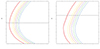 |
Fig. 4. As in Fig. 2, but assuming [Fe/H] = −0.3 as reference. Dashed tracks have [Fe/H] = −0.2. |
| In the text | |
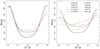 |
Fig. 5. As in Fig. 1, but assuming [Fe/H] = −0.3 as reference. |
| In the text | |
Current usage metrics show cumulative count of Article Views (full-text article views including HTML views, PDF and ePub downloads, according to the available data) and Abstracts Views on Vision4Press platform.
Data correspond to usage on the plateform after 2015. The current usage metrics is available 48-96 hours after online publication and is updated daily on week days.
Initial download of the metrics may take a while.