| Issue |
A&A
Volume 687, July 2024
|
|
|---|---|---|
| Article Number | A177 | |
| Number of page(s) | 9 | |
| Section | Catalogs and data | |
| DOI | https://doi.org/10.1051/0004-6361/202348885 | |
| Published online | 09 July 2024 | |
Metallicities for more than 10 million stars derived from Gaia BP/RP spectra★
1
Zentrum für Astronomie der Universität Heidelberg, Landessternwarte,
Königstuhl 12,
69117
Heidelberg,
Germany
e-mail: txylaki@lsw.uni-heidelberg.de
2
Department of Astronomy, Stockholm University, AlbaNova University Center,
SE-106 91
Stockholm,
Sweden
3
Research School of Astronomy and Astrophysics, Australian National University,
Canberra,
ACT 2611,
Australia
4
ARC Centre of Excellence for All Sky Astrophysics in 3 Dimensions (ASTRO 3D),
Australia
5
George P. and Cynthia Woods Mitchell Institute for Fundamental Physics and Astronomy, Texas A&M University,
College Station,
TX
77843,
USA
6
Department of Physics & Astronomy, Texas A&M University,
4242 TAMU, College Station,
TX
77843,
USA
Received:
8
December
2023
Accepted:
10
March
2024
Context. The third Gaia Data Release, which includes BP/RP spectra for 219 million sources, has opened a new window into the exploration of the chemical history and evolution of the Milky Way. The wealth of information encapsulated in these data is far greater than their low resolving power (R ~ 50) would suggest at first glance, as shown in many studies. We zeroed in on the use of these data for the purpose of the detection of “new” metal-poor stars, which are hard to find yet essential for understanding several aspects of the origin of the Galaxy, star formation, and the creation of the elements, among other topics.
Aims. We strive to refine a metal-poor candidate selection method that was developed with simulated Gaia BP/RP spectra with the ultimate objective of providing the community with both a recipe to select stars for medium and high resolution observations, and a catalog of stellar metallicities.
Methods. We used a dataset comprised of GALAH DR3 and SAGA database stars in order to verify and adjust our selection method to real-world data. For that purpose, we used dereddening as a means to tackle the issue of extinction, and then we applied our fine-tuned method to select metal-poor candidates, which we thereafter observed and analyzed.
Results. We were able to infer metallicities for GALAH DR3 and SAGA stars with color excesses up to E(B − V) < 1.5 and an uncertainty of σ[Fe/H]inf ∼ 0.36, which is good enough for the purpose of identifying new metal-poor stars. Further, we selected 26 metal-poor candidates via our method for observations. As spectral analysis showed, 100% of them had [Fe/H] < −2.0, 57% had [Fe/H] < −2.5, and 8% had [Fe/H] < −3.0. We inferred metallicities for these stars with an uncertainty of σ[Fe/H]inf ∼ 0.31, as was proven when comparing [Fe/H]inf to the spectroscopic [Fe/H]. Finally, we assembled a catalog of metallicities for 10 861 062 stars.
Key words: catalogs / surveys / stars: Population II
Full Table 3 is available at the CDS via anonymous ftp to cdsarc.cds.unistra.fr (130.79.128.5) or via https://cdsarc.cds.unistra.fr/viz-bin/cat/J/A+A/687/A177
© The Authors 2024
 Open Access article, published by EDP Sciences, under the terms of the Creative Commons Attribution License (https://creativecommons.org/licenses/by/4.0), which permits unrestricted use, distribution, and reproduction in any medium, provided the original work is properly cited.
This article is published in open access under the Subscribe to Open model. Subscribe to A&A to support open access publication.
1 Introduction
The oldest stars that are still alive today and located nearby have metallicities of less than −3 (Beers & Christlieb 2005). These extremely metal-poor (EMP) stars are rare and difficult to find. They are the descendants of the first generation of stars. Hence, EMP stars carry information that can shed light on the properties of their predecessors as well as on how the latter exploded and ended their lives. Consequently, finding a large number of new EMP stars for which detailed studies of their chemical composition could be conducted is of the essence since such investigations would provide constraints on the assembly of the Galaxy, on the initial mass function of the first stars, and on the nucleosynthesis processes that formed the heavy elements. The Gaia Survey (Gaia Collaboration 2023) released in 2022 the low-resolution (R ~ 50) Gaia BP/RP spectra for 219 million sources (De Angeli et al. 2023), and there have already been many studies that have provided metallicity estimates for several thousands to millions of objects by extracting information from BP/RP spectra, often with the use of additional data from Gaia itself (for example Radial Velocity Spectrometer (RVS) spectra; Katz et al. 2023) or other surveys. Bellazzini et al. (2023) derived metallicities for ~700 000 stars, and Andrae et al. (2023a) delivered a catalog of stellar parameters, including the metallicity, using a Bayesian forward-modeling approach (Bailer-Jones et al. 2013). Yao et al. (2024) used a classification algorithm, XGBoost (Chen & Guestrin 2016), to identify 188 000 very metal-poor star candidates. Rix et al. (2022) used the machine learning algorithm XGBoost to estimate [M/H] for 2 million stars, with 18 000 of them in the very- and metal-poor regime. Andrae et al. (2023b) produced a new catalog that improved on the one of Rix et al. (2022). The new catalog was assembled by training the XGBoost algorithm on stellar parameters taken from the Data Release 17 (DR17) of the Sloan Digital Sky Survey’s (SDSS) APOGEE survey (Abdurro’uf et al. 2022) and from Li et al. (2022), who derived stellar parameters for 400 extremely and ultra metal-poor stars. Andrae et al. (2023b) delivered a catalog for ~ 175 million stars, with a mean precision of 0.1 dex for [M/H]. Zhang et al. (2023) used a forward model to estimate the effective temperature, surface gravity, metallicity, distance, and extinction for 220 million stars. In order to do so, they used the Gaia XP-based data-driven models along with 2MASS (Skrutskie et al. 2006) and WISE (Schlafly et al. 2019) photometry. The forward model was then trained and validated on stellar parameters from the LAMOST survey (Wang et al. 2022), yielding [Fe/H] with a typical uncertainty of 0.15 dex. Martin et al. (2023) used the BP/RP spectra to derive synthetic photometry of the Ca H & K region based on the narrow-band photometry of the Pristine Survey (Starkenburg et al. 2017). They updated the Pristine metallicity inference model so that it is exclusively based on Gaia magnitudes (G, GBP, and Grp) and produced a catalog of metallicities for more than 52 million stars. Martin et al. (2023) showed that their photometric metallicities are accurate down to [Fe/H] ~ −3.5 and are thus very much suited for the study of the metal-poor Galaxy. Another study that took advantage of the BP/RP spectra in order to derive stellar parameters and/or metallicities is Cunningham et al. (2024).
Xylakis-Dornbusch et al. (2022) (Paper I) developed an empirical method based on flux ratios of synthetic Gaia BP/RP spectra for the purpose of identifying new metal-poor stars. Specifically, the flux ratios were those of the Ca H & K lines to the Hβ region (frCaHK/Hβ with 388 nm < λ < 401 nm and 479 nm < λ < 501 nm) and the G-band region to the Ca near-infrared (NIR) triplet (frG/CaNIR with 420 nm < λ < 444 nm and 846 nm < λ < 870 nm). It was shown that for a roughly constant frG/CaNIR, the frCaHK/Hβ exponentially declines as metallicity increases. This work is a follow-up to Paper I and aims at verifying the metal-poor star selection recipe presented therein by applying it to Gaia DR3 BP/RP spectra. The paper is laid out in the following manner: in Sec. 2 we describe the dataset we used for the purpose of validating the method in Paper I as well as how we addressed the issue of extinction, which was not dealt with in our previous work. We close the section with a description of the modifications we performed on the selection procedure and metallicity estimation of the metal-poor candidate stars compared to that introduced in Paper I. Next, we present in Sec. 3 the results of the method verification, including the expected success rate in selecting stars that are very metal poor ([Fe/H] < −2) and below this threshold and the purity of that ensemble. Then we investigate the plausibility of OBA stars being selected as metal-poor stars via our method. Furthermore, in Sec. 5 we describe the application of our fine-tuned recipe by selecting candidate metal-poor stars and subsequently observing them. We then present the results of our observations. Finally, in Sec. 6 we present a catalog of metallicities including stars in both the metal-poor and metal-rich regimes.
2 Methods
For the verification of the selection process, we used stellar parameters from high- and medium-resolution surveys and studies along with the respective flux dereddened Gaia BP/RP spectra. The software GaiaXPy1 was used to generate the Gaia BP/RP spectra, and dust_extinction2 and dustmaps3 (Green 2018) were used to deredden the spectral flux.
2.1 Dataset
The dataset we used for this work is comprised of two different cross-matches with Gaia BP/RP externally calibrated spectra (Gaia Collaboration 2023, Montegriffo et al. 2023). The first cross-match was with the Stellar Abundances for Galactic Archaeology (SAGA) database (Suda et al. 2008, 2011; Yamada et al. 2013; Suda et al. 2017), and the second was with the Galactic Archaeology with HERMES data release 3 (GALAH DR3) (Buder et al. 2021). Both datasets together consist of 21 812 stars. We applied quality cuts on the aforementioned dataset by finding correlations between falsely identified metal-poor stars and quality parameters and ended up with 20 850 stars. Since this procedure could only be done after the application of our method to the dataset, we elaborate on it in both this section as well as in the results section. The quality cuts we applied were twofold: one with respect to the quality of the stellar parameters of the dataset and another stemming from the quality of the Gaia BP/RP spectra themselves as well as from the effect of reddening. Concerning the first, stars for which there was no reliable metallicity estimate from GALAH were dropped (flag_fe_h=0). The mean uncertainty in the iron abundance for the remaining GALAH stars is 0.12 dex. We did not use any quality flag for the SAGA stars, but we resorted to the provided iron abundance uncertainties ![$\[\left(\bar{\sigma}_{\mathrm{SAGA}} \sim 0.17 \mathrm{dex}\right)\]$](/articles/aa/full_html/2024/07/aa48885-23/aa48885-23-eq3.png) . The GALAH [Fe/H] were computed using A(Fe)⊙ = 7.38 (for details see Buder et al. 2021), while the SAGA database utilizes the Asplund et al. (2009) solar chemical composition, that is, A(Fe)⊙ = 7.50. We considered this difference in the normalization of the metallicities of the two components comprising our dataset to be negligible since our aim is not to deliver high-precision iron abundances but rather to identify metal-poor stars. Further, as appears in the Kiel Diagram (Fig. 1), the final dataset we used spans from dwarf to giant stars, with most of the GALAH stars having disk-like kinematics (Buder et al. 2021) and a mean distance of
. The GALAH [Fe/H] were computed using A(Fe)⊙ = 7.38 (for details see Buder et al. 2021), while the SAGA database utilizes the Asplund et al. (2009) solar chemical composition, that is, A(Fe)⊙ = 7.50. We considered this difference in the normalization of the metallicities of the two components comprising our dataset to be negligible since our aim is not to deliver high-precision iron abundances but rather to identify metal-poor stars. Further, as appears in the Kiel Diagram (Fig. 1), the final dataset we used spans from dwarf to giant stars, with most of the GALAH stars having disk-like kinematics (Buder et al. 2021) and a mean distance of ![$\[\bar{D} \sim 1.9\]$](/articles/aa/full_html/2024/07/aa48885-23/aa48885-23-eq4.png) kpc (distances taken from Bailer-Jones et al. 2018) and the SAGA stars having
kpc (distances taken from Bailer-Jones et al. 2018) and the SAGA stars having ![$\[\bar{D} \sim 1.8\]$](/articles/aa/full_html/2024/07/aa48885-23/aa48885-23-eq5.png) kpc (distances taken from Fouesneau et al. 2023) and belonging to the Galactic halo. Regarding the spectra quality, we set a limit to the blending fraction β of the BP/RP spectra and the color excess (E(B − V)). The former was defined by Riello et al. (2021) as “... the sum of the number of blended transits in BP and RP divided by the sum of the number of observations in BP and RP.” We slightly modified the definition to
kpc (distances taken from Fouesneau et al. 2023) and belonging to the Galactic halo. Regarding the spectra quality, we set a limit to the blending fraction β of the BP/RP spectra and the color excess (E(B − V)). The former was defined by Riello et al. (2021) as “... the sum of the number of blended transits in BP and RP divided by the sum of the number of observations in BP and RP.” We slightly modified the definition to
β = (bp_n_blended_transits + rp_n_blended_transits+
bp_n_contaminated_transits + rp_n_contaminated_transits)/
(bp_n_transits + rp_n_transits),
and we set β ≤ 0.5. Finally, complementary to our work in Paper I, we included objects in our dataset whose reddening is well above E(B − V) = 0.06 (see Fig. 2), which mandates that we tackle the issue of extinction.
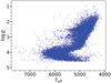 |
Fig. 1 Kiel diagram of the dataset. |
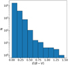 |
Fig. 2 Histogram of the reddening distribution of our dataset. |
2.2 Reddening
As a first approach, we aimed at finding a reddening independent index, similar to Bonifacio et al. (2000a). Since the region of the Hβ line is part of the frCaHK/Hβ ratio (see Paper1 for details), we decided to test if the Strömgren β index withstands extinction and replaced the Hβ region in frCaHK/Hβ with the former. The results were not what we had anticipated: The β index changed with extinction, even though it showed a sensitivity to effective temperature. As we were not able to define a reddening-independent metallicity calibration, we instead sought to implement reddening corrections for the metallicity calibration by means of dereddening the spectra. Therefore, we used the dust maps of Schlegel et al. (1998) (SFD) re-calibrated by Schlafly & Finkbeiner (2011), the extinction model of Fitzpatrick (1999), and Rυ = 3.1 to deredden the externally calibrated BP/RP spectra. We repeated the above procedure using the extinction model of Cardelli et al. (1989) and found that the resulting flux ratios have minimal differences with those calculated with the Fitzpatrick (1999) model. We chose the SFD maps because they cover the entire sky. Considering the fact that the SFD maps account for the foreground dust, our stars needed to be distant enough or at a galactic latitude great enough for the distance dependence to be neglected. The SAGA stars are halo stars and are thus distant enough (D ≥ 1 kpc; Schlafly & Finkbeiner 2011). In total, 81% of the stars in our dataset are either at a distance of D≥1 kpc or at a latitude of | b |> 30°. For the remaining 19%, we calculated the reddening correction from Bonifacio et al. (2000b). For most of the stars, we found no or a very small (<0.001 mag) correction. Only for 4% of the total sample, we found E(B − V) corrections ≥0.02 mag, so applying such a correction would have a negligible effect on the distribution in the dereddened flux-ratio plane (Fig. 3).
2.3 Application of the method
In Paper I, we provided coefficients for different pairs of Teff and log g for the estimation of [Fe/H]. We calibrated the coefficients for application to the real data, but the results did not correspond to the theoretical expectations. Further, the problem of acquiring well-defined effective temperatures and surface gravities for millions of stars so that the metal-poor ones among them could be identified became apparent. We decided to use only quantities that could be directly derived from the spectra (i.e. the flux ratios). The plane of the frCaHK/Hβ and frG/CaNIR flux ratios (see Fig. 3) enabled us to find the loci of metal-poor ([Fe/H] < −1.0) and further metal-deficient stars. The gray lines in Fig. 3 represent different metallicity regimes, with the stars below the dashed-dotted and dotted lines being metal poor ([Fe/H] < − 1) and very metal poor ([Fe/H] < − 2), respectively.
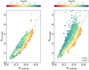 |
Fig. 3 Flux ratios of raw (left panel) and dereddened (right panel) fluxes from Gaia BP/RP spectra. The color-coding reflects the metal-licity of the stars of the dataset we used. Below the dashed-dotted and dotted lines are the flux-ratio areas where stars with [Fe/H] ≤ −1 and [Fe/H] ≤ −2, respectively, are primarily found. |
3 Results
The results in the right panel of Fig. 3 depict a clear correlation between metallicity frCaHK/Hβ and frG/CaNIR flux ratios. The left panel shows the flux ratios before dereddening, and the right panel shows the dereddened values. We overplotted a dashed-dotted line (Cutoff1) and a dotted line (Cutoff2) to designate flux-ratio areas where objects with [Fe/H]ref ≤ −1 and [Fe/H]ref ≤ −2, respectively, are primarily found ([Fe/H]ref is the reference [Fe/H]). By selecting metal-poor stars in this way, we found that there was a correlation between a high blending fraction β and contaminants (i.e. stars with [Fe/H]ref > −1). We chose the β such that there is a balance between acceptable contamination and completeness since a greater β means a greater number of stars. We defined the completeness as the ratio of the number of selected stars below a certain metallicity threshold to the total number of stars in the dataset that have [Fe/H]ref ≤ threshold, the success rate as the percent of the selected stars that have [Fe/H]ref below a certain specified value, and the contamination as the percent of selected stars that have a metallicity above the specified threshold.
The results in Fig. 3 were generated after the application of the quality cuts described above. By choosing all the stars below Cutoff1 in Fig. 3, we were able to recover from the GALAH-SAGA sample more than 98% of the stars with [Fe/H] ≤ − 2, all the ultra metal-poor stars ([Fe/H] ≤ −4), and 70% of the stars [Fe/H] < −1. We recorded a success rate of ~80%, 44%, and 20% for stars with [Fe/H] ≤ −1, −1.5, and −2, respectively. When we selected stars below Cutoff2, we made a trade-off between the success rate and the completeness. We still recovered more than 90% and 94% of the very and extremely metal-poor stars, respectively, but we lost about 40% of those with − 2 < [Fe/H] ≤ − 1 compared to the other Cutoff1. The success rate increased significantly to ~99%, 95%, and 60% for stars with [Fe/H] ≤ −1, −1.5, and −2, respectively (summarized in Fig. 4). As before, we selected all the stars that fell below the same dotted and dashed-dotted line without dereddening (left panel of Fig. 3) for comparison and calculated the statistics as above. Even though the completeness for different metallicity categories is fairly similar and in some cases even slightly better, the success rate is much lower, and consequently, the contamination is much higher.
Further, we found that by selecting the metal-poor candidates through the flux-ratio plane, we could extrapolate the theoretical method described in Paper I to a broader parameter space. Specifically, the recipe in Paper I was developed for FGK stars in the effective temperature range of 4800–6300 K, and in this study, we retrieved metal-poor stars that have 4636 K ≤ Teff ≤ 7150 K.
Finally, we estimated the iron abundances of our dataset as follows. First, we randomly sampled our GALAH-SAGA dataset and split it into two equal parts. We divided the flux ratios of the first sampled sub-dataset into frG/CaNIR bins. Then, we split each of those bins into metallicity bins, for which we calculated the mean frCaHK/Hβ. Next, we found the best fits to the sets of frCaHK/Hβ−[Fe/H] pairs (Fig. 5), which we subsequently used to estimate the iron abundance of the second sub-dataset. We used the following function to perform the fittings:
![$\[f r_{\mathrm{G} / \mathrm{CaNIR}}=-a \cdot f r_{\mathrm{CaHK} / \mathrm{H} \beta}{ }^b+c,\]$](/articles/aa/full_html/2024/07/aa48885-23/aa48885-23-eq6.png) (1)
(1)
where a, b, and c are the coefficients of the best fit, which are shown in Table 1. The respective results of the metallicity estimation are presented in Fig. 6. We were able to infer [Fe/H] with an uncertainty of ![$\[\sigma_{[\mathrm{Fe} / \mathrm{H}]_ \mathrm{inf}} \sim 0.36\]$](/articles/aa/full_html/2024/07/aa48885-23/aa48885-23-eq7.png) dex. This precision is sufficient to reliably identify metal-poor stars.
dex. This precision is sufficient to reliably identify metal-poor stars.
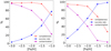 |
Fig. 4 Completeness, success rate, and contamination of the stars that were selected from below the dashed-dotted (left panel) and dotted line (right panel). The stars were selected from a dereddened flux-ratio plane. |
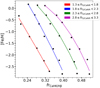 |
Fig. 5 Best fits to the frCaHK/Hβ-[Fe/H] pairs. The different line colors convey the frG/CaNIR range of applicability. |
Coefficients of the best fit.
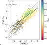 |
Fig. 6 Metallicity estimation of a subset of the GALAH-SAGA dataset. The points that have a black circle around them are located below the black-dotted line in the flux-ratio plane (Fig. 3). The color-coding reflects the effective temperature of the stars. We plotted the inferred and reference [Fe/H] on the x- and y-axis respectively. |
4 OBA stars
OBA stars are young hot stars that can present emission lines in their spectra. When OB stars are highly reddened, they can appear as K-type stars. Hence, good reddening values are essential to tell them apart from metal-poor FGK stars. Also, young or accreting stars can show emission lines at various spectral regions, including the Ca H&K absorption lines. Consequently, the emission in the Ca II H&K lines results in a net weak absorption line that masks these stars as metal poor. Therefore, we wished to test to which degree those stars are expected to contaminate a selected metal-poor candidate sample.
We selected a random subset of 200 stars from the OBA stars’ golden sample4. From those, 193 stars have an externally calibrated BP/RP spectrum, and 173 have a blending fraction β ≤ 0.5. We dereddened the externally calibrated spectra as described in Sec. 2.2 and subsequently computed the flux ratios. In Fig. 7, we plot the flux ratios of the OBA golden sample subset. In order to show the effect of extinction, which depends on the color excess rather than on the flux ratios, we used logarithmic axes. The effect of extinction is indicated with an arrow (orange arrow), where its nock and point represent the flux ratios before and after dereddening, respectively, for E(B − V) ≈ 0.3 mag. As can be seen, none of the 173 stars appear in the region of the flux-ratio plane where the metal-poor stars are frequently found (Fig. 3). However, due to the fact that the location of the stars on the flux-ratio plane depends on the extinction, we caution the reader that highly reddened OBA stars with underestimated color-excess values could appear in the region of metal-poor stars (yellow area in Fig. 7) and hence contaminate the sample of metal-poor stars selected via this method.
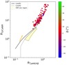 |
Fig. 7 Flux ratios of OBA stars. The solid and dotted lines represent Cutoff1 and Cutoff2, respectively, while the yellow shaded area designates the region that is populated by very metal-poor stars (see Fig. 3). The color-coding indicates the Galactic Latitude b of each star. As can be seen, most of the stars are located on the Galactic plane (| b |≤ 10°). The orange arrow illustrates the effect of extinction for a color excess E(B − V) ≈ 0.3 mag. The nock and the point of the arrow represent the flux ratios before and after dereddening, respectively. |
5 Observational metal-poor star candidate verification
In order to verify our metal-poor candidate selection method as well as the metallicity estimation presented herein, we selected a sample of stars from Gaia DR3 that had not been observed before. We opted to select fairly bright giant stars in order to achieve a good enough signal-to-noise ratio (S/N) for the purpose of deriving precise [Fe/H]. Further, the location of the telescope to be used was known beforehand; hence we used the following selection criteria: G = 12–13 mag, Ra = 16–02 h, Dec = 00° to +20°, | b |> 20°, and β ≤ 0.5, which rendered 90 798 stars. We then computed the flux ratios. From the 90 798 stars, we chose those with flux ratios of 1 ≤ frG/CaNIR ≤ 5, which left us with 70 509 stars. Next, we selected all the stars below a more stringent cut than Cutoff2, which is a line that is shifted parallel to Cutoff2 by 0.1+frCaHK/Hβ. This cutoff left us with 77 stars, of which ten had already been observed in high resolution, and their metallicities are, or will be, in the literature. It is worth noting that all ten of the stars that appear in literature are metal poor. The reason we used a more stringent cut was that there is a clear correlation between the inferred metallicity and the position of the star on the flux-ratio plane. We opted to observe candidates with the lowest predicted metallicities, as if we had used Cutoff2, most of the stars above the more stringent cutoff would not have made it into the final target list due to the higher estimated [Fe/H]inf. We show the distribution of the inferred [Fe/H]inf for metal-poor candidates that were located between Cutoff2 and our chosen cutoff in Fig. A.1. Finally, we estimated the [Fe/H] for the remaining 67 stars, and our final target list was comprised of 32 stars with [Fe/H]inf ≤ −2.35, of which we managed to observe 26. Of the 35 stars that were not included in the target list, eight of them were outside the metallicity inference range (frG/CaNIR > 3.3). The distribution of the inferred metallicities for the remaining 27 metal-poor candidates that were not included in the final target list is shown in Fig. A.2.
5.1 Observations and metallicity determinations
The targets were observed at the McDonald Observatory with the Harlan J. Smith 2.7 m telescope and the TS23 echelle spectrograph (Tull et al. 1995). The spectra were obtained using a 1.2″ slit and 1x1 binning, yielding a resolving power of R ~ 60,000 and covering a wavelength range of 3600–10 000 Å. The 26 stars were observed over four nights in August 2023. The data was reduced using standard IRAF packages (Tody 1986, 1993), including correction for bias, flat-field, and scattered light. Table 2 lists the Gaia DR3 id, right ascension, declination, Heliocentric Julian Date (HJD), exposure times, the S/N per pixel at 5000 Å and heliocentric radial velocities. The heliocentric radial velocities were determined via cross-correlation with a spectrum of the standard star HD 182488 (Vhel = −21.2 km s−1; Soubiran et al. (2018)) obtained on the same run.
We determined the stellar parameters (Teff, log g, [Fe/H], and υt) for the observed stars from a combination of photometry and equivalent width (EW) measurements of Fe <sc>I</sc> and Fe <sc>II</sc> lines and using the software smhr5 (Casey 2014) to run the radiative transfer code MOOG6 (Sneden 1973; Sobeck et al. 2011), assuming local thermodynamical equilibrium. We used one dimensional plane-parallel α-enhanced ([α/Fe] = +0.4) stellar model atmospheres computed from the ATLAS9 grid (Castelli & Kurucz 2003) and line lists from linemake7 (Placco et al. 2021). Solar abundances were taken from Asplund et al. (2009), and Teff for the stars was determined from dereddened Gaia G, BP, RP (Anders et al. 2022; Gaia Collaboration 2018), and 2MASS K magnitudes (Cutri et al. 2003) using the color-Teff relations from Mucciarelli et al. (2021). For the K magnitudes, we used the extinction coefficient from McCall (2004). The log g was then determined by requiring ionization equilibrium between the Fe <sc>I</sc> and Fe <sc>II</sc> lines and υt by requiring no correlation of the Fe <sc>I</sc> line abundances with reduced EW. Finally, the [Fe/H]spec of the stars was taken as the mean abundances of the Fe I lines, and the uncertainties are the standard deviation of these. The final stellar parameters are listed in Table 2.
5.2 Results
The stellar parameters of the observed stars are shown in Table 2. As the parameters show, all observed stars are metal-poor FGK stars. The uncertainty in our metallicity inference is ![$\[\sigma_{[\mathrm{Fe} / \mathrm{H}]_ \mathrm{inf}} \sim 0.31\]$](/articles/aa/full_html/2024/07/aa48885-23/aa48885-23-eq8.png) , which agrees with the uncertainty in deriving metallicities for the GALAH-SAGA sample (
, which agrees with the uncertainty in deriving metallicities for the GALAH-SAGA sample (![$\[\sigma_{[\mathrm{Fe} / \mathrm{H}]_ \mathrm{inf}} \sim 0.36\]$](/articles/aa/full_html/2024/07/aa48885-23/aa48885-23-eq9.png) ), as described above. Figure 8 shows [Fe/H]inf versus the spectroscopic-determined [Fe/H]spec. Further, 100% of the observed stars are very metal-poor, 58% have [Fe/H] < −2.5, and 8% are EMP. Lastly, we did not have any contamination from OBA stars, which agrees with our finding in Sec. 4.
), as described above. Figure 8 shows [Fe/H]inf versus the spectroscopic-determined [Fe/H]spec. Further, 100% of the observed stars are very metal-poor, 58% have [Fe/H] < −2.5, and 8% are EMP. Lastly, we did not have any contamination from OBA stars, which agrees with our finding in Sec. 4.
6 Catalog of stellar [Fe/H]
For the purpose of providing the community with a catalog of metallicities, we used the following criteria from The Milky Way Halo High-Resolution Survey (Christlieb et al. 2019) of the 4-meter Multi-Object Spectroscopic Telescope (4MOST) (De Jong et al. 2019) combined with the criteria developed for this work to select stars from Gaia DR3: | b | > 10°, 0.15 mag ≤ (BP − RP)0 < 1.1 mag, blending index β ≤ 0.5, 1.3 ≤ frG/CaNIR ≤ 3.3, and E(B − V) ≤ 1.5 mag. These criteria yielded 10 861 062 stars, for which we estimated the metallicity. We note that 225 498 stars in this catalog have [Fe/H]inf < − 2. 0. Further, in our catalog, 2236 stars have [Fe/H]inf < − 5. 0, which suggests that these stars probably have emission lines rather than being metal-poor. We cross-matched the stars of our catalog that have [Fe/H]inf < − 2. 0 with the Gaia OBA golden sample (European Space Agency (ESA) & DPAC Consortium 2022), and we found that 104 of the stars are indeed OBA stars. Out of those OBA contaminants, eight have an estimated metallicity [Fe/H]inf < −5.0 in the catalog. A sample of the catalog is shown in Table 3.
Stellar parameters and observation log of observed metal-poor candidates.
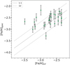 |
Fig. 8 [Fe/H]inf versus [Fe/H]spec. The solid gray line is the 1 to 1 line, and the dashed gray line designates the 1σ uncertainty ( |
![$\[\sigma_{[\mathrm{Fe} / \mathrm{H}]_{\text {spec }}}\]$](/articles/aa/full_html/2024/07/aa48885-23/aa48885-23-eq11.png)
7 Comparison to other catalogs
As already described in the introduction, many studies have taken advantage of the wealth of information encapsulated in the Gaia BP/RP spectra and have provided to the community catalogs of stellar atmospheric parameters. Specifically, the catalogs of Andrae et al. (2023b) and Martin et al. (2023) have been shown to work very well in the metal-poor regime. We used the GALAH-SAGA verification sub-dataset (Fig. 6) to compare the metallicities we estimated versus those of Andrae et al. (2023b) and Martin et al. (2023). The [Fe/H]inf we estimated for this sub-dataset are independent of the fitting procedure. Figure 9 shows the performance of each catalog. At first glance, it is clear that the catalog of Martin et al. (2023) performs better in the metal-poor regime than ours and that of Andrae et al. (2023b). However, the difference in accuracy of the inferred metallicities in all three catalogs is comparable. Specifically for [Fe/H]ref < −2, the iron abundances of Martin et al. (2023) and Andrae et al. (2023b) have σ ~ 0.39 and are 0.1 dex better than ours. For [Fe/H]ref < −3, the standard deviation of the estimated metallicities in all three catalogs is the same, that is, ~0.36 dex. In the metal-rich regime, our metallicities have uncertainties that are ~0.2 dex higher than those of the other two catalogs, whose performance is similar, σ ~ 0.24 dex.
8 Summary
We applied the metal-poor star candidate selection recipe described in Paper I (Xylakis-Dornbusch et al. 2022) to Gaia DR3 BP/RP spectra. In order to do so, we updated the selection method. Specifically, instead of using the effective temperature and surface gravity information, we only used the flux ratios, frG/CaNIR and frCaHK/Hβ, determined in Paper I to estimate the metallicity of the stars. We addressed the extinction by means of dereddening the spectra before computing the flux ratios, and we found that the method can be applied to stars with color excesses E(B − V) ≤ 1.5. We then used BP/RP spectra through a crossmatch between Gaia DR3 and GALAH DR3 as well as with the SAGA database to validate the selection method. We were able to estimate the [Fe/H] solely with the use of the flux ratios, with an uncertainty of ![$\[\sigma_{[\mathrm{Fe} / \mathrm{H}]_{\mathrm{inf}}} \sim 0.36\]$](/articles/aa/full_html/2024/07/aa48885-23/aa48885-23-eq12.png) dex. Next, we assessed to which degree OBA stars could contaminate a metal-poor candidate sample selected via the method described herein. We found that it is not very likely as long as one has a high level of color excesses at their disposal to perform the dereddening of the spectra. Following this, we selected stars from Gaia DR3 via our updated selection procedure for spectroscopic validation. We observed 26 stars, of which 100% had [Fe/H] < −2.0, 58% had [Fe/H] < −2.5, and 8% had [Fe/H] < −3.0. We inferred the metallicites for this sample of stars prior to observations with an uncertainty
dex. Next, we assessed to which degree OBA stars could contaminate a metal-poor candidate sample selected via the method described herein. We found that it is not very likely as long as one has a high level of color excesses at their disposal to perform the dereddening of the spectra. Following this, we selected stars from Gaia DR3 via our updated selection procedure for spectroscopic validation. We observed 26 stars, of which 100% had [Fe/H] < −2.0, 58% had [Fe/H] < −2.5, and 8% had [Fe/H] < −3.0. We inferred the metallicites for this sample of stars prior to observations with an uncertainty ![$\[\sigma_{[\mathrm{Fe} / \mathrm{H}]_{\mathrm{inf}}} \sim 0.31\]$](/articles/aa/full_html/2024/07/aa48885-23/aa48885-23-eq13.png) dex. Finally, we assembled a catalog of metallicities for 10 861 062, of which 225 498 have [Fe/H]inf < −2.0.
dex. Finally, we assembled a catalog of metallicities for 10 861 062, of which 225 498 have [Fe/H]inf < −2.0.
Sample of the catalog of metallicities.
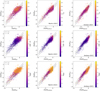 |
Fig. 9 Comparison of our derived metallicities with those from the Andrae et al. (2023b) (XGBOOST) and Martin et al. (2023) (CaHKsynth) catalogs. Top (from left to right): Metallicities of our, XGBOOST, and CaHKsynth catalogs are plotted, respectively, for the GALAH-SAGA validation dataset ([Fe/H]ref). The color-coding reflects the effective temperature of the stars. Middle and bottom: same as the top panels but the color-coding depicts the color excess and surface gravity, respectively. The solid black line shows the 1–1 line, while the dashed lines show a σ = 0.36 dex uncertainty. |
Acknowledgements
We thank the anonymous referee for their comments, which helped improve this manuscript. This work was funded by the Deutsche Forschungsgemeinschaft (DFG, German Research Foundation) – Project-ID 138713538 – SFB 881 (“The Milky Way System”, subproject A04). This research was supported by the Australian Research Council Centre of Excellence for All Sky Astrophysics in 3 Dimensions (ASTRO 3D), through project number CE170100013. This work was supported by computational resources provided by the Australian Government through the National Computational Infrastructure (NCI) under the National Computational Merit Allocation Scheme and the ANU Merit Allocation Scheme (project y89). TXD acknowledges support from the Heidelberg Graduate School for Physics (HGSFP). TTH acknowledges support from the Swedish Research Council (VR 2021-05556). This work made use of the Third Data Release of the GALAH Survey (Buder et al. 2021). The GALAH Survey is based on data acquired through the Australian Astronomical Observatory, under programs: A/2013B/13 (The GALAH pilot survey); A/2014A/25, A/2015A/19, A2017A/18 (The GALAH survey phase 1); A2018A/18 (Open clusters with HERMES); A2019A/1 (Hierarchical star formation in Ori OB1); A2019A/15 (The GALAH survey phase 2); A/2015B/19, A/2016A/22, A/2016B/10, A/2017B/16, A/2018B/15 (The HERMES-TESS program); and A/2015A/3, A/2015B/1, A/2015B/19, A/2016A/22, A/2016B/12, A/2017A/14 (The HERMES K2-follow-up program). We acknowledge the traditional owners of the land on which the AAT stands, the Gamilaraay people, and pay our respects to elders past and present. This paper includes data that has been provided by AAO Data Central (https://www.datacentral.org.au). This work has made use of data from the European Space Agency (ESA) mission Gaia (https://www.cosmos.esa.int/gaia), processed by the Gaia Data Processing and Analysis Consortium (DPAC, https://www.cosmos.esa.int/web/gaia/dpac/consortium). Funding for the DPAC has been provided by national institutions, in particular the institutions participating in the Gaia Multilateral Agreement. This work has made use of the Python package GaiaXPy, developed and maintained by members of the Gaia Data Processing and Analysis Consortium (DPAC) and in particular, Coordination Unit 5 (CU5), and the Data Processing Centre located at the Institute of Astronomy, Cambridge, UK (DPCI).
Appendix A Additional figures
We present additional figures that are described in Section 5. We show the inferred metallicity distribution of the candidate metal-poor stars that are located on the flux-ratio plane between Cutoff2 and the more stringent cut we used to select stars for observations. Lastly, we show the metallicity distribution of the metal-poor candidates below the stringent cutoff not included in the target list.
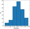 |
Fig. A.1 Distribution of [Fe/H]inf for metal-poor candidates located between Cutoff2 and the cutoff we used to select candidates for observations. |
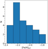 |
Fig. A.2 Distribution of [Fe/H]inf of the 27 metal-poor candidates that were not included in the final target list. |
References
- Abdurro’uf, Accetta, K., Aerts, C., et al. 2022, ApJS, 259, 35 [NASA ADS] [CrossRef] [Google Scholar]
- Anders, F., Khalatyan, A., Queiroz, A. B. A., et al. 2022, A&A, 658, A91 [NASA ADS] [CrossRef] [EDP Sciences] [Google Scholar]
- Andrae, R., Fouesneau, M., Sordo, R., et al. 2023a, A&A, 674, A27 [CrossRef] [EDP Sciences] [Google Scholar]
- Andrae, R., Rix, H.-W., & Chandra, V. 2023b, ApJS, 267, 8 [NASA ADS] [CrossRef] [Google Scholar]
- Asplund, M., Grevesse, N., Sauval, A. J., & Scott, P. 2009, ARA&A, 47, 481 [NASA ADS] [CrossRef] [Google Scholar]
- Bailer-Jones, C. A. L., Andrae, R., Arcay, B., et al. 2013, A&A, 559, A74 [NASA ADS] [CrossRef] [EDP Sciences] [Google Scholar]
- Bailer-Jones, C. A. L., Rybizki, J., Fouesneau, M., Mantelet, G., & Andrae, R. 2018, AJ, 156, 58 [Google Scholar]
- Beers, T. C., & Christlieb, N. 2005, ARA&A, 43, 531 [NASA ADS] [CrossRef] [Google Scholar]
- Bellazzini, M., Massari, D., De Angeli, F., et al. 2023, A&A, 674, A194 [NASA ADS] [CrossRef] [EDP Sciences] [Google Scholar]
- Bonifacio, P., Caffau, E., & Molaro, P. 2000a, A&AS, 145, 473 [NASA ADS] [CrossRef] [EDP Sciences] [Google Scholar]
- Bonifacio, P., Monai, S., & Beers, T. C. 2000b, AJ, 120, 2065 [Google Scholar]
- Buder, S., Sharma, S., Kos, J., et al. 2021, MNRAS, 506, 150 [NASA ADS] [CrossRef] [Google Scholar]
- Cardelli, J. A., Clayton, G. C., & Mathis, J. S. 1989, ApJ, 345, 245 [Google Scholar]
- Casey, A. R. 2014, PhD thesis, Australian National University, Canberra, Australia [Google Scholar]
- Castelli, F., & Kurucz, R. L. 2003, in Modelling of Stellar Atmospheres, 210, eds. N. Piskunov, W. W. Weiss, & D. F. Gray, A20 [Google Scholar]
- Chen, T., & Guestrin, C. 2016, in Proceedings of the 22nd ACM SIGKDD International Conference on Knowledge Discovery and Data Mining, KDD ’16 (ACM) [Google Scholar]
- Christlieb, N., Battistini, C., Bonifacio, P., et al. 2019, The Messenger, 175, 26 [NASA ADS] [Google Scholar]
- Cunningham, E. C., Hunt, J. A. S., Price-Whelan, A. M., et al. 2024, ApJ, 963, 95 [NASA ADS] [CrossRef] [Google Scholar]
- Cutri, R. M., Skrutskie, M. F., van Dyk, S., et al. 2003, VizieR Online Data Catalog: II/246 [Google Scholar]
- De Angeli, F., Weiler, M., Montegriffo, P., et al. 2023, A&A, 674, A2 [NASA ADS] [CrossRef] [EDP Sciences] [Google Scholar]
- De Jong, R. S., Agertz, O., Berbel, A. A., et al. 2019, The Messenger, 175, 3 [NASA ADS] [Google Scholar]
- European Space Agency (ESA) & DPAC Consortium 2022, Gaia DR3 source IDs of O, B, and A-type stars, https://doi.org/10.17876/gaia/dr.3/59 [Google Scholar]
- Fitzpatrick, E. L. 1999, PASP, 111, 63 [Google Scholar]
- Fouesneau, M., Frémat, Y., Andrae, R., et al. 2023, A&A, 674, A28 [NASA ADS] [CrossRef] [EDP Sciences] [Google Scholar]
- Gaia Collaboration (Prusti, T., et al.) 2023, A&A, 595, A1 [Google Scholar]
- Gaia Collaboration (Babusiaux, C., et al.) 2018, A&A, 616, A10 [NASA ADS] [CrossRef] [EDP Sciences] [Google Scholar]
- Gaia Collaboration (Vallenari, A., et al.) 2023, A&A, 674, A1 [NASA ADS] [CrossRef] [EDP Sciences] [Google Scholar]
- Green, G. 2018, J. Open Source Softw., 3, 695 [NASA ADS] [CrossRef] [Google Scholar]
- Katz, D., Sartoretti, P., Guerrier, A., et al. 2023, A&A, 674, A5 [NASA ADS] [CrossRef] [EDP Sciences] [Google Scholar]
- Li, H., Aoki, W., Matsuno, T., et al. 2022, ApJ, 931, 147 [NASA ADS] [CrossRef] [Google Scholar]
- Martin, N. F., Starkenburg, E., Yuan, Z., et al. 2023, A&A submitted [arXiv:2308.01344] [Google Scholar]
- McCall, M. L. 2004, AJ, 128, 2144 [Google Scholar]
- Montegriffo, P., De Angeli, F., Andrae, R., et al. 2023, A&A, 674, A3 [NASA ADS] [CrossRef] [EDP Sciences] [Google Scholar]
- Mucciarelli, A., Bellazzini, M., & Massari, D. 2021, A&A, 653, A90 [NASA ADS] [CrossRef] [EDP Sciences] [Google Scholar]
- Placco, V. M., Sneden, C., Roederer, I. U., et al. 2021, RNAAS, 5, 92 [NASA ADS] [Google Scholar]
- Riello, M., De Angeli, F., Evans, D. W., et al. 2021, A&A, 649, A3 [NASA ADS] [CrossRef] [EDP Sciences] [Google Scholar]
- Rix, H.-W., Chandra, V., Andrae, R., et al. 2022, ApJ, 941, 45 [NASA ADS] [CrossRef] [Google Scholar]
- Schlafly, E. F., & Finkbeiner, D. P. 2011, ApJ, 737, 103 [Google Scholar]
- Schlafly, E. F., Meisner, A. M., & Green, G. M. 2019, ApJS, 240, 30 [Google Scholar]
- Schlegel, D. J., Finkbeiner, D. P., & Davis, M. 1998, ApJ, 500, 525 [Google Scholar]
- Skrutskie, M. F., Cutri, R. M., Stiening, R., et al. 2006, AJ, 131, 1163 [NASA ADS] [CrossRef] [Google Scholar]
- Sneden, C. A. 1973, PhD thesis, University of Texas, Austin, USA [Google Scholar]
- Sobeck, J. S., Kraft, R. P., Sneden, C., et al. 2011, AJ, 141, 175 [NASA ADS] [CrossRef] [Google Scholar]
- Soubiran, C., Jasniewicz, G., Chemin, L., et al. 2018, A&A, 616, A7 [NASA ADS] [CrossRef] [EDP Sciences] [Google Scholar]
- Starkenburg, E., Martin, N., Youakim, K., et al. 2017, MNRAS, 471, 2587 [NASA ADS] [CrossRef] [Google Scholar]
- Suda, T., Katsuta, Y., Yamada, S., et al. 2008, PASJ, 60, 1159 [NASA ADS] [Google Scholar]
- Suda, T., Yamada, S., Katsuta, Y., et al. 2011, MNRAS, 412, 843 [NASA ADS] [Google Scholar]
- Suda, T., Hidaka, J., Aoki, W., et al. 2017, PASJ, 69, 76 [Google Scholar]
- Tody, D. 1986, SPIE Conf. Ser., 627, 733 [Google Scholar]
- Tody, D. 1993, ASP Conf. Ser., 52, 173 [NASA ADS] [Google Scholar]
- Tull, R. G., MacQueen, P. J., Sneden, C., & Lambert, D. L. 1995, PASP, 107, 251 [NASA ADS] [CrossRef] [Google Scholar]
- Wang, C., Huang, Y., Yuan, H., et al. 2022, ApJS, 259, 51 [NASA ADS] [CrossRef] [Google Scholar]
- Xylakis-Dornbusch, T., Christlieb, N., Lind, K., & Nordlander, T. 2022, A&A, 666, A58 [NASA ADS] [CrossRef] [EDP Sciences] [Google Scholar]
- Yamada, S., Suda, T., Komiya, Y., Aoki, W., & Fujimoto, M. Y. 2013, MNRAS, 436, 1362 [Google Scholar]
- Yao, Y., Ji, A. P., Koposov, S. E., & Limberg, G. 2024, MNRAS, 527, 10937 [Google Scholar]
- Zhang, X., Green, G. M., & Rix, H.-W. 2023, MNRAS, 524, 1855 [NASA ADS] [CrossRef] [Google Scholar]
Software available at https://gaia-dpci.github.io/GaiaXPy-website/, https://doi.org/10.5281/zenodo.7566303
All Tables
All Figures
|
Fig. 1 Kiel diagram of the dataset. |
| In the text | |
|
Fig. 2 Histogram of the reddening distribution of our dataset. |
| In the text | |
|
Fig. 3 Flux ratios of raw (left panel) and dereddened (right panel) fluxes from Gaia BP/RP spectra. The color-coding reflects the metal-licity of the stars of the dataset we used. Below the dashed-dotted and dotted lines are the flux-ratio areas where stars with [Fe/H] ≤ −1 and [Fe/H] ≤ −2, respectively, are primarily found. |
| In the text | |
|
Fig. 4 Completeness, success rate, and contamination of the stars that were selected from below the dashed-dotted (left panel) and dotted line (right panel). The stars were selected from a dereddened flux-ratio plane. |
| In the text | |
|
Fig. 5 Best fits to the frCaHK/Hβ-[Fe/H] pairs. The different line colors convey the frG/CaNIR range of applicability. |
| In the text | |
|
Fig. 6 Metallicity estimation of a subset of the GALAH-SAGA dataset. The points that have a black circle around them are located below the black-dotted line in the flux-ratio plane (Fig. 3). The color-coding reflects the effective temperature of the stars. We plotted the inferred and reference [Fe/H] on the x- and y-axis respectively. |
| In the text | |
|
Fig. 7 Flux ratios of OBA stars. The solid and dotted lines represent Cutoff1 and Cutoff2, respectively, while the yellow shaded area designates the region that is populated by very metal-poor stars (see Fig. 3). The color-coding indicates the Galactic Latitude b of each star. As can be seen, most of the stars are located on the Galactic plane (| b |≤ 10°). The orange arrow illustrates the effect of extinction for a color excess E(B − V) ≈ 0.3 mag. The nock and the point of the arrow represent the flux ratios before and after dereddening, respectively. |
| In the text | |
|
Fig. 8 [Fe/H]inf versus [Fe/H]spec. The solid gray line is the 1 to 1 line, and the dashed gray line designates the 1σ uncertainty ( |
| In the text | |
|
Fig. 9 Comparison of our derived metallicities with those from the Andrae et al. (2023b) (XGBOOST) and Martin et al. (2023) (CaHKsynth) catalogs. Top (from left to right): Metallicities of our, XGBOOST, and CaHKsynth catalogs are plotted, respectively, for the GALAH-SAGA validation dataset ([Fe/H]ref). The color-coding reflects the effective temperature of the stars. Middle and bottom: same as the top panels but the color-coding depicts the color excess and surface gravity, respectively. The solid black line shows the 1–1 line, while the dashed lines show a σ = 0.36 dex uncertainty. |
| In the text | |
|
Fig. A.1 Distribution of [Fe/H]inf for metal-poor candidates located between Cutoff2 and the cutoff we used to select candidates for observations. |
| In the text | |
|
Fig. A.2 Distribution of [Fe/H]inf of the 27 metal-poor candidates that were not included in the final target list. |
| In the text | |
Current usage metrics show cumulative count of Article Views (full-text article views including HTML views, PDF and ePub downloads, according to the available data) and Abstracts Views on Vision4Press platform.
Data correspond to usage on the plateform after 2015. The current usage metrics is available 48-96 hours after online publication and is updated daily on week days.
Initial download of the metrics may take a while.