| Issue |
A&A
Volume 685, May 2024
|
|
|---|---|---|
| Article Number | A105 | |
| Number of page(s) | 11 | |
| Section | Celestial mechanics and astrometry | |
| DOI | https://doi.org/10.1051/0004-6361/202348378 | |
| Published online | 15 May 2024 | |
Secular evolution of resonant planets in the coplanar case
Application to the systems HD 73526 and HD 31527
Departamento de Astronomía, Instituto de Física, Facultad de Ciencias,
UdelaR, Iguá 4225,
Montevideo
11400,
Uruguay
e-mail: This email address is being protected from spambots. You need JavaScript enabled to view it.
; This email address is being protected from spambots. You need JavaScript enabled to view it.
Received:
24
October
2023
Accepted:
18
January
2024
Abstract
Aims. We study the secular evolution of two planets in mutual deep mean-motion resonance (MMR) in the planar elliptic three-body problem framework for different mass ratios. We do not consider any restriction in the eccentricity of the inner planet e1 or in the eccentricity of the outer planet e2.
Methods. The method we used is based on a semi-analytical model that consists of calculating the averaged resonant disturbing function numerically. It is assumed for this that all the orbital elements (except for the mean longitudes) of both planets are constant on the resonant timescale. In order to obtain the secular evolution inside the MMR, we make use of the adiabatic invariance principle, assuming a zero-amplitude resonant libration. We constructed two phase portraits, called the ℋ1 and ℋ2 surfaces, in the three-dimensional spaces (e1, Δϖ, σ) and (e2, Δϖ, σ), where Δϖ is the difference between the planetary longitude of perihelia and σ is the critical angle. These surfaces, which are related through the angular moment conservation, allow us to find the apsidal corotation resonances (ACRs) and to predict the secular evolution of e1, e2, Δϖ, and σ (libration center).
Results. While studying the 1:1, 2:1, 3:1, and 3:2 MMR, we found that large excursions in eccentricity can exist in some particular cases. We compared the secular variations of e1, e2, Δϖ, and σ predicted by the model with a numerical integration of the exact equations of motion for different mass ratios. We obtained good matches. Finally, the model was applied to study the secular evolution of the resonant exoplanet systems HD 73526 and HD 31527. They both have a pair of planets and are very close to the deep MMR condition. In the first system, we found that the pair of planets that constitutes the system evolves in a symmetrical ACR, whereas in the second system, we found that planets c and d, which are in an unusual 16:3 MMR, are close to an ACR, but outside its dynamical region, where Δϖ circulates.
Key words: methods: numerical / celestial mechanics / planets and satellites: dynamical evolution and stability
© The Authors 2024
 Open Access article, published by EDP Sciences, under the terms of the Creative Commons Attribution License (https://creativecommons.org/licenses/by/4.0), which permits unrestricted use, distribution, and reproduction in any medium, provided the original work is properly cited.
This article is published in open access under the Subscribe to Open model. This email address is being protected from spambots. You need JavaScript enabled to view it. to support open access publication.
1 Introduction
The long-term dynamical evolution of planetary systems is defined by what is called their secular dynamics. Some planetary systems are occasionally known to be in mean-motion resonance (MMR), which means that their orbital periods are related in a simple way. The secular dynamics of planetary systems within MMR are generally very different from those outside MMR (Beaugé & Michtchenko 2003; Callegari et al. 2004; Batygin & Morbidelli 2013).
Methods for studying the secular dynamics of planetary systems within an MMR must initially contemplate and correctly reproduce the dynamics of the MMR. Some methods for planetary systems in MMR have been developed using analytical methods (Batygin & Morbidelli 2013; Quillen & French 2014), some were pure numerical studies (Haghighipour et al. 2003), and semi-analytical methods were also proposed (Michtchenko et al. 2008; Gallardo et al. 2021).
The secular evolution of planetary systems within MMRs is a more challenging problem (Batygin & Morbidelli 2013). The restricted problem is a simpler case, that is, a particle that is perturbed by an unperturbed planet. In our first paper (Pons & Gallardo 2022), we proposed a method for following the secular dynamics of a particle in deep resonance (i.e., zero libration amplitude) with a planet. In this paper, we generalize the method to the study of a two-planet system in deep MMR, allowing us to obtain the long-term evolution of the planetary system without restrictions on the eccentricity.
This work is organized as follows. Section 2 describes the theoretical framework, starting with the Hamiltonian formalism, the calculation formulae for the equilibrium points, and a brief description of the invariant adiabatic principle that allows the application of the model on secular timescales. Then, Sect. 3 describes the method we used to apply the model in the most generic and comprehensive way. There, we recall the definition and construction of the phase-space graphical representation we call ℌ surface. Finally, we describe some nomenclature that we used to distinguish and classify the apsidal corrota-tion resonances (ACRs). Section 4 presents the most interesting results. This section is divided into two subsections, the first of which presents the generic results found for 1:1, 2:1, 3:1, and 3:2 MMRs, and the second subsection contains the results we achieved by applying the model to two real exoplanetary systems. In Sect. 5, we present our conclusions.
2 Theoretical framework
2.1 Semi-analytical theory
As is commonly used, index 1 is reserved for the inner and index 2 for the outer planet. This means that a1 ≤ a2. Index 0 is reserved for the star. The method we describe in this work is valid for coplanar orbits of planets in deep MMR with arbitrary masses. In order to obtain some simplified expressions below, we assume that m1,2 << m0.
Following the model developed by Gallardo et al. (2021), we can express the canonical elements of the planets in a coplanar configuration as follows:
 (1)
(1)
where βi = m0mi/(m0 + mi) is the reduced mass, µi = k2(m0 + mi), ai is the ith planet semi-major axis, ei is the eccentricity, and k is the gravitational Gauss constant. With these variables, the Hamiltonian takes the next form,
 (2)
(2)
where R is the disturbing function, which can be expressed in the following way:
 (3)
(3)
Here, ri, vi are the planetary position and velocities in the Poincare reference system. The nonperturbative Hamiltonian is given by the term ℌ0 = H + R.
Our next step is to introduce the so-called critical angle σ = k1λ1 − k2 λ2 + (k2 − k1 )ϖ1. In order to do so, we apply a canonical transformation (see Appendix A) and obtain the following set of canonical variables:
 (4)
(4)
This transformation also introduces the variable ∆ϖ = ϖ1 − ϖ2, which is useful for studying the ACRs in planetary systems (Beaugé et al. 2003; Michtchenko et al. 2008).
To conclude the basis of our theoretical development, we calculate the averaged disturbing function 𝓡 (see Appendix A) following the approach given in Gallardo (2020), that is, we make an average in λ2 assuming that on the resonant timescale (which is longer than the timescale on which the average is performed) a1, a2, e1, e2, and ∆ϖ remain constant. This is a good approximation as long as the eccentricities are not too close to 0, because the closer they are to 0, the larger the longitudes of the perihelion change rate.
After the averaging, the Hamiltonian no longer depends on λ2. Therefore, I2 becomes a constant of motion, correlating the evolution of the semi-major axis. Additionally, when we apply D’Alembert rules to a generic argument of the form ϕ = k1λ1 + k2λ2 + k3ϖ1 + k4ϖ2, it can be demonstrated that 𝓡 depends on σ and ∆ϖ, but not on ϖ2, implying that 𝓚2 is another constant of motion. Based on these arguments, the Hamiltonian takes the following form:
 (5)
(5)
where all the values before the semicolon are variables, and all values after the semicolon are considered fixed parameters. These dependences of the resonant Hamiltonian variables are valid on secular timescales.
2.2 Equilibrium points
Under the assumption of deep MMR condition, the two semi-major axis are constant, that is, L1 and L2 are also constant (see Sect. 2.3). In addition, on resonant timescales, as we previously stated, e1, e2, and ∆ϖ can also be considered constant, that is, 𝓚1 and 𝓚2 are constant. This allows us to write that
 (6)
(6)
where I1 = I1nom (where nom stands for nominal, which refers to the values for the exact resonance, given by Eq. (8)), and the remaining values after the semicolon are considered fixed parameters, at least on the resonant timescale. We consider I1 to be a variable in the nonperturbative term, but a constant in the perturbative term. This manipulation does not change the results and simplifies the search for the equilibrium point.
To obtain the equilibrium points under these further assumptions, we used the canonical equations. Therefore, we have that the equilibrium points must satisfy the following conditions:
 (7)
(7)
The first equation leads to n1k1 = n2k2, where ni describes the planetary mean motions. This is the deep resonant condition, which is equivalent to the following formula:
 (8)
(8)
where for a given a2, a1 is defined by the masses and by the MMR k2:k1 . We refer to this value as the nominal semi-major axis of the resonance.
The second equation indicates that all the equilibrium points are located in the extrema of the 𝓡(σ) function. In particular, it can be demonstrated (see Appendix A) that the stable equilibrium points occur in the minima of this function. We assume that a minimum occurs in σn. Therefore, we can say that there is an stable equilibrium point in (I1, σ) = (I1nom, σn). In resonant dynamics, the stable equilibrium points are also known as libra-tion centers. In general, for a given set of (a1, a2, e1, e2, ∆ϖ), N ≥ 1 libration centers (I1nom, σn) can exist with n = 1…N. For better graphical representations, we occasionally use an alternative for the critical angle, which is defined as follows:
 (9)
(9)
A priori, all libration centers are valid. Nevertheless, when a close encounter between the planets occurs, the evolution can become unstable, leading to strong changes in the orbital elements, including ai. This implies that the MMR is broken. In order to dismiss these stable equilibrium points in the encounter condition, we use Hill’s criteria. Consequently, we disregard a libration center when the following condition is met:
 (10)
(10)
where RHill is the planetary Hill radius, which is defined as follows (Gladman 1993):
 (11)
(11)
For practical use, we chose in general a ξ value from 3 to 4, depending on the particular studied case. A more complete analysis of ξ values can be found in Gallardo et al. (2021).
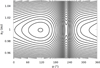 |
Fig. 1 Averaged resonant Hamiltonian contour curves in plane (a2, σ) in 3:1 MMR for a system with m1 = m2, e1 = 0,47, e2 = 0,38, and ∆ϖ = 84°. |
2.3 Secular model
With the purpose of deriving a model that is applicable to secular timescales, we used the adiabatic invariant principle. In the celestial mechanics context, in particular, in planetary dynamics, this principle states that as long as the variations in ei and ∆ϖ are slow enough, a quantity J exists that is related to faster variables (I1 and σ). This variable remains constant in time. This quantity is known as the adiabatic invariant and is defined as follows:
 (12)
(12)
This definition can be interpreted as the enclosed area inside one of the curves of the Hamiltonian level shown in Fig. 1. The mathematical details of which exactly mean that the variations in ei and ∆ϖ are slow enough can be found in Henrard (1993). In simple terms, we assumed that ei and ∆ϖ change much more slowly (i.e., adiabatically) than I1 and σ.
For practical reasons, we assumed the ideal case of J = 0, as in Pons & Gallardo (2022). This implies that the area of the enclosed curve in the (I1 ,σ) plane is 0. In other words, we are located exactly in the libration center. In this situation, the planetary resonant angles librate around the equilibrium value, but with null resonant amplitude, which describes the deep MMR hypothesis we mentioned in Sect. 2.1.
The value of a given libration center σn can change as a consequence of ei and ∆ϖ variations (we recall Eqs. (6) and (7)) that are present in the secular evolution. When no encounter occurs, the adiabatic invariant principle ensures that the system continues in a deep MMR condition.
3 Method
3.1 AMD conservation
Since we have that 𝓚2 is a constant of motion and L1 is assumed constant (because of the deep MMR hypothesis), we conclude that −(Γ1 + Γ2) is also constant. This is the quantity known as angular momentum deficit (AMD), which is defined as follows (Laskar 1997):
 (13)
(13)
Petit et al. (2017) concluded that in the presence of MMR, there is no guarantee that AMD is conserved. This is mainly due to the chaos that emerges when an MMR overlap occurs, particularly in high-eccentricity domains. We assumed that there is no MMR overlapping, which is reasonable in the deep-resonance hypothesis. In other words, we assumed that AMD is conserved even in a MMR.
3.2 Eccentricity domain
If the AMD is conserved, then the following quantity is also conserved:
 (14)
(14)
This quantity becomes the angular momentum of the system when m1,2 << m0 (Michtchenko et al. 2008). Regardless of the case, 𝒜𝓜 always has the same functional form, which is
 (15)
(15)
where  are constants because they only depend on the masses and semi-major axis (which are constant because of the deep MMR hypothesis). It is convenient to define a normalized 𝒜𝓜 as follows:
 (16)
(16)
where 𝒜𝓜max = C1 + C2, and η = C2/C1 is a new parameter we defined. With some simple operations, we obtained
 (17)
(17)
where the last equality is valid only when m1,2 << m0. In this condition, the functional form of 𝒜𝓜norm only depends on the planetary mass ratio and on the MMR in which the masses are locked. Figure 2 shows an example of the 𝒜𝓜norm function and its contour curves. These curves allow a rapid identification of the eccentricity domains, that is, the possible variation ranges of e1 and e2.
In order to inclusively and generically study the secular dynamics of resonant coplanar planets with eccentric orbits, we assumed 𝒜𝓜norm and η as free parameters. A priori, a double sweep in these two parameters might be performed. Nevertheless, in the context of planetary dynamics, we considered a predefined set of MMRs and a set of mass ratios that determined the values for η. On the one hand, the MMR set comprised the most typical and stronger resonances, which are the 2:1, 3:2, 3:1, and 1:1 MMR. For the ratio m2/m1, we considered the values 1/20, 1/5, 1, 5, and 20. From the combination of these two sets, we obtained 20 different values for η that ranged from 0.5 to almost 30. On the other hand, the 𝒜𝓜norm values were chosen (after η was defined) after an inspection of the contour curves, with the aim of selecting the cases for which a higher eccentricity excursion appeared possible. This condition was usually met for 𝒜𝓜norm values between 0.7 to 0.95. We present the most interesting cases hereafter studying all those that resulted from our selection criteria.
After 𝒜𝓜norm was fixed, the value of one eccentricity determined that of the other. For instance, for a value of e1, e2 is given by the formula below,
![Mathematical equation: ${e_2} = \sqrt {1 - {{\left[ {\left( {1 + {\eta ^{ - 1}}} \right){\cal A}{{\cal M}_{{\rm{norm }}}} - {\eta ^{ - 1}}\sqrt {1 - e_1^2} } \right]}^2}} .$](/articles/aa/full_html/2024/05/aa48378-23/aa48378-23-eq19.png) (18)
(18)
This equation allows drawing two restrictions. The first restriction emerges just from the fact that the term inside the radicals must be positive. Therefore,
 (19)
(19)
The second restriction arises when we inspect the term inside the straight parentheses in expression (18). This term must be also positive because if it is not, the second term in Eq. (16) would be negative. For this reason, we have
 (20)
(20)
These two limiting conditions for the eccentricity variation ranges are useful in the next section, when we detail the method we used to explore the phase space.
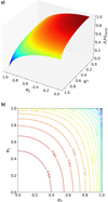 |
Fig. 2 Normalized angular momentum function 𝒜𝓜norm(e1, e2) for 2:1 MMR with m2 = m1. (a) Three-dimensional plot of 𝒜𝓜norm(e1, e2). (b) 𝒜𝓜norm(e1, e2) contour curves with numerical values above the curves. |
3.3 ℌ surfaces
Exploiting the fact that we work with conservative systems, we constructed some phase portraits that are very useful because they contain the constant Hamiltonian contour curves. When a system has more than one degree of freedom, these phase portraits are constructed considering one coordinate and its conjugate momenta as variables and the rest as parameters. In our case, the averaged Hamiltonian has three degrees of freedom a priori, which translates into six variables that essentially are a1, a2, e1, e2, ϖ1, and ϖ2. On the one hand, as a result of the deep MMR condition, a1 and a2 were assumed constant, and as we mentioned previously, 𝓡 depends on Am and σ (not on ϖ1 and ϖ2 separately). On the other hand, AM conservation allows us to establish a relation between e1 and e2. Therefore, we have essentially three variables of interest to understand the secular evolution in the resonant context, which are ei (where the index i takes the value 1 or 2), ∆ϖ, and σ. For the three variables, we used the graphical representation developed by Pons & Gallardo (2022). This representation allows us to build one single phase portrait that contains all the information of the secular evolution of the system instead of several bidimensional phase portraits with one of the three variables as a parameter. The single phase portrait containing all the information is called 𝓗 surface.
Pons & Gallardo (2022) introduced the 𝓗 surface for the restricted case of the coplanar and resonant three-body problem. In the present research, we need two 𝓗 surfaces, one for each planet. Consequently, one surface is associated with the variables (e1, ∆ϖ, σ), and the other surface with (e2, ∆ϖ, σ). We call these phase portraits surface 𝓗1 and surface 𝓗2. They are related through the 𝒜𝓜 conservation because this condition relates e1 with e2 (we recall expression (15)). As a consequence, the topology of the two surfaces is the same, but they can vary somewhat in size or scale. For this reason, it is usually sufficient to study one of them to understand the system evolution qualitatively.
3.4 Apsidal corotation resonances
In terms of secular evolution, there are two possible behaviors for the angular variable Am. The first behavior is circulation, where ∆ϖ eventually takes on all the possible values for an angular variable and essentially maintains the same sign as the time derivative. Alternatively, ∆ϖ can librate (or oscillate) around a certain value. In this last case, the two planets are in ACR (Beaugé et al. 2003; Zhou et al. 2004). If this libration has null amplitude, the angle between each the line of the apsides of each orbit is fixed and the two eccentricities also remain unchanged. The situation in which each orbit is frozen with respect to the other persists until some external mechanism removes the planets from the exact ACR point.
The ACRs are classified into two groups: symmetric ACRs, and the asymmetric ACRs. The symmetric ACRs occur when ∆ϖ is 0° or 180°. In asymmetric ACRs, ∆ϖ takes the remaining possible angular values. This ACR distinction is very frequently used in the literature. Is reasonable that asymmetric ACR have double multiplicity because of the geometrical symmetry of the problem, as we explain next. When the orientation of one orbit with respect to the other implies that the relative position between them is frozen on secular timescales, then the evolution should be the same when we consider a new configuration of the orientation, making an axial symmetry with respect to the symmetry of the apsis lines. Moreover, the planetary position in the orbit should also be symmetrical to the line of aspsis. The mathematical counterpart of these statements is that when M is the mean anomaly, when an ACR exists in (∆ϖ, M1) = (∆ϖα, M1α) (we assumed M2 = 0°), then another ACR exists in (∆ϖ, M1) = (−∆ϖα, −M1α). With some simple operations, the same holds for the critical angle, that is, when the first ACR has σ = σα, then the other ACR has σ = −σα. A numerical example would be that when an ACR exists in ∆ϖ = 45° and σ = 60°, then another asymmetric ACR must exist in ∆ϖ= 360 − 45 = 315° and σ = 360 − 60 = 300° (here we summed 360° just to work with positive values). In order to simplify the ACR count, we always refer to a group of two ACRs as one asymmetric ACR.
We introduce another criterion below to classify ACRs in the framework of resonant dynamics. ACR type I or ACRI are ACRs with a fixed libration center on the secular timescale. Conversely, ACR type II or ACRII are ACRs with a changing libration center on secular timescale (in all studied cases, this change was always of a circulation type, but there is no reason a priori that prevents it from having a librational-type change in the nominal value of the ACR). In this case, the exact ACR may coincide with the edge of an 𝓗 surface. This implies that a system in an exact ACRII cannot possibly maintain invariant J because it is too close to the edge of the 𝓗 surface (Pons & Gallardo 2022).
3.5 Numerical integrations
To perform numerical integrations, we made use of the Mer-curius algorithm included in the Rebound Python package, which is a hybrid symplectic integrator that is very similar to Mercury (Chambers 1999). It is basically composed of a WHFast algorithm that switches over smoothly to IAS15 whenever a close encounter occurs.
4 Results and discussion
4.1 General results
Without losing generality, we fixed some variables to explore the phase space. For the rest of the work, we have a2 = 1 au and a larger planet with mass mi = 1 MJ.
With the aim of testing and validating the model, we compared every phase portrait presented in this paper with numerical integrations of the exact equations of motion. A small correction was sometimes required to the initial value for a1 given by Eq. (8) in order to ensure the deep MMR condition. This is mainly due to the short-term perturbations and to the law of structure (Ferraz-Mello 1988), which can slightly modify the resonant nominal semi-major axis. The MMR we studied first is presented below. In some of the integrations, we had to implement these corrections to ensure the zero-amplitude condition in the resonant librations.
4.1.1 MMR 2:1
In panel a of Fig. 3, we show two examples of 𝓗 surfaces, both regarding a planetary system locked in 2:1 MMR with 𝒜𝓜norm = 0.9. The first system is a planetary system with m2/m1 = 0.2. In this case, there are two topologically separated surfaces in the phase portrait. When this occurs, we name them subsurfaces. One of the subsurfaces has a constant libration center (θ = 0°) and an ACRI in (e2, ∆ϖ, θ) = (0.88, 180°, 0°). The contour curves of the constant Hamiltonian are plotted in black, and the five numerical integrations run to test the model are shown in red (some initial a1 values were modified up to 7% from the nominal value to obtain the deep MMR condition). Two integrations were required in the case of apsidal corotation resonance, and three were required with a circulating ∆ϖ.
The other subsurface contains an asymmetric ACRI located near ∆ϖ= θ = 0° (see the red marker in panel b of Fig. 3) and for a lower eccentricity value. In this particular case, the subsurface was filtered to remove areas in which a close encounter might occur. In one of these encounter zones lay another asymmetric ACRI. However, as expected, numerical integrations with initial conditions in this zone resulted in a chaotic evolution. Similar to the other subsurface, we show in colors five 1 kyr numerical integrations, four of which are in ACR condition (but around the two close ACR points) and the remaining one is in a ∆ϖ circulating condition. This last integration shows a great e2 excursion of at least 0.6 (green curve).
The second case presented here for the MMR 2:1 is a system with m2/m1 = 1. Figure 3b shows the resulting 𝓗1 surface. Here, four ACR type I are distributed in two subsurfaces. Due to the circularity of the angular variables, it seems to be more than two. Notwithstanding, there are only two topologically separated subsurfaces. This time, nine numerical integrations were performed to compare with the model. Most of them were evolutions around an ACR, except for one (yellow curve), with a circulating ∆ϖ. The assymetric ACR with an integation in green is in a quasi-encounter situation because at this point |r2 − r1| ≃ 4RHill. This integration is stable, but for a displacement from the ACR initial conditions, the evolution remains stable for 400 yr at most and then shows an irregular behavior.
We recall that three topological types of constant 𝓗 curves are possible in these surfaces: closed ones with a librating ∆ϖ (ACR condition), closed ones with a circulating ∆ϖ, and open curves (Pons & Gallardo 2022). The last type of curves implies a breach of the invariance principle that might hamper the comparison between the model and the numerical experiments and might in some cases lead to chaotic behavior. All the initial conditions of the numerical integrations shown here correspond to the first two groups of curves. The yellow curve is at the limit of being in a closed curve. If the initial e1 were increased slightly, the evolution changes drastically turning into a chaotic behavior because an open curve family lies on the surface.
We found that the model contour curves and the numerical integrations in all the cases presented so far agree well. This is not a strictly mathematical proof that the model is correct, but it contributes to validating the model.
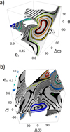 |
Fig. 3 Phase portraits for MMR 2:1 and 𝒜𝓜norm = 0.9. (a) 𝓗2 surface for a system with m2/m1 = 0.2. The ten numerical integrations run for 10 kyr are plotted in colors (some areas of the surface were removed for clarity). (b) 𝓗1 surface for a system with m2/m1 = 1. The nine numerical integrations run for 1 kyr are shown. |
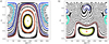 |
Fig. 4 𝓗1 (e1, ∆ϖ) contour curves for the 3:2 MMR for two different systems. (a) First system: m2/m1 = 1 and 𝒜𝓜norm = 0.95. (b) Second system: m2/m1 = 5 and 𝒜𝓜norm = 0.9. In both panels, the numerical integrations are drawn in color. The red crosses indicate the initial condition in each case. |
4.1.2 MMR 3:2
In this section, we present two examples in MMR 3:2. The first example consists of a planetary system with m2/m1 = 1 and 𝒜𝓜norm = 0.95. We focused on the secular evolution of e1 and ∆ϖ and consequently disregarded the evolution of the libration center. This was achieved by projecting the 𝓗1 surface onto the (e1, ∆ϖ) plane. The result of this operation is shown in Fig. 4. In particular, panel a of the figure shows the evolution of the system. Two symmetric ACRs are visible. One is located in ∆ϖ= 180° and the other in ∆ϖ= 0°. The last ACR is type II and is placed inside the encounter zone, and therefore, the contour curves in the proximity of the ACR are missing. In this case in particular, surface areas where |r2 − r1 | < 4.5RHill were removed. The evolution in an encounter zone in general is related to abrupt variations in the semi-major axis (which obviously disrupt the resonant condition) and strong changes in eccentricity, which can lead to a collision with the star or to an ejection from the system. In between the two ACRs lies a transition zone where ∆ϖ circulates.
The second system is characterized by m2/m1 = 5 and 𝒜𝓜norm = 0.9. In this case, the dynamical structure is more complex, as shown in Fig. 4b. It shows four symmetric ACRs, three of which are type I, and the remaining ACR is type II. The transition areas between ACRs seem to be distorted because 𝓗1 overlaps slightly with itself. This constitutes a practical problem when a projection is intended.
The numerical integration and the model contour curves in the two systems again agree well. In these examples, eccentricity excursions up to 0.4 at least can occur.
4.1.3 MMR 3:1
As in the previous MMRs, we present two examples for the 3:1 MMR as well. The phase-space structure is shown in Fig. 5. Panel a shows the phase portrait of a system with two equal-mass planets and 𝒜𝓜norm = 0.8. The resulting 𝓗1 surface is similar to the surface shown in Fig. 3a because in both cases, a symmetric ACRI and an asymmetric ACRI lie close to ∆ϖ= σ = 0°. They differ basically in the position of the eccentricity value.
The second example consists of a system with m2/m1 = 0.2 and 𝒜𝓜norm = 0.99. This time, there is an asymmetric ACRI and, for lower e1 values, a symmetric ACRII around which the libration center circulates on secular timescales.
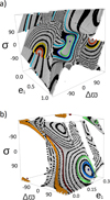 |
Fig. 5 Phase portraits for MMR 3:1. (a) 𝓗1 surface for a system with m2/m1 = 1 and 𝒜𝓜norm = 0.8. The ten numerical integrations run for 10 kyr are plotted in colors. (b) 𝓗1 surface for a system with m2/m1 = 0.2 and 𝒜𝓜norm = 0.99. The five numerical integrations run for 1 kyr are shown. |
4.1.4 MMR 1:1
From all the cases investigated in this MMR, we present the most interesting, which consists of a system with m2 = m1 and 𝒜𝓜norm = 0.9. In this case, there are three subsurfaces with negligible libration center variation, that is, which are essentially planes located at σ ~ 0°, σ ~ 120° and σ ~ 240°. We therefore present just the Hamiltonian contour curves projected onto the (ei, ∆ϖ) domain. On the one hand, in Fig. 6a, we show the contour curves of the case σ ~ 120° , where two asymmetric ACRI lie. We only show this subsurface, but the other sub-urface around σ ~ 240°, has a similar aspect, but is flipped symmetrically with respect to the ∆ϖ= 0° axis. This ACR distribution completely satisfies the explanation given in Sect. 3.4 for the pair multiplicity in all asymmetric ACRs. On the other hand, in Fig. 6b, we show a stable symmetric ACRI (the other one is in encounter condition). These five ACRs correspond to the classical Lagrangian solutions L3, L4, and L5 and to the two points mentioned as anti-Lagrangian points in Giuppone et al. (2010, see Table 1 of that work). There, the authors carried out a very complete research in co-orbital planetary motion, where they explored the entire ACR families for different m2/m1 values.
4.2 Real exoplanetary systems
After investigating the secular dynamics of coplanar resonant three-body systems with a generic approach, we explored the exoplanet database1 to find examples of resonant planet pairs with the aim of applying the model to them. Our intention was to focus on systems that might be in or near the deep MMR condition and with at least one planet with moderate to high eccentricity. In order to meet these criteria, we disregarded systems with a resonant offset (Charalambous et al. 2022) larger than 2%. Additionally, we filtered the database and selected systems with at least one planet with e > 0.2 and with a low uncertainty in their determination (∆e < 0. 05). After we searched the database, we found 22 exoplanet pairs. Most of them were analyzed, and we finally selected two of the more interesting systems. The first system is in a very common resonance, but in a deep MMR condition. The second system is in a very rare MMR and also very close to the deep MMR condition.
For a real exoplanet system locked in a k2 : k1 MMR, we calculated the 𝒜𝓜norm from its planetary masses, semi-major axes, and eccentricities. The procedure of the 𝓗 surface construction was then analogous to the generic case. Finally, a numerical integration of the real system was carried out, and the result was compared directly with the 𝓗 surface contour curves.
For a given system, the initial conditions used for the numerical integration were obtained from the orbital elements for which observational data were fit. In the following sections, the corresponding paper is referenced for each analyzed system. At the moment of setting up the numerical integration, some adjustments to the initial conditions were needed for a more straightforward comparison with our model. On the one hand, our model focuses in the relative orientation of the orbits, that is, it considers ∆ϖ to describe the orientation. We therefore assumed ϖ2 = 0° and calculated ϖ1 = ϖ1i − ϖ2i, where variables with the subindex i refer to the data obtained from the original paper.
On the other hand, we also redefined the reference zero time by imposing M2 = 0°. This implies that M1 = (τ2i − τ1i) * (360°/P1), where P1 is the orbital period of the inner planet, and τ is the time of periapsis passage. For each system, we finally summarized the orbital elements in a table where we also compare the libration center value σ given by the model with the real value σint given by the orbital elements of the system, in order to be quantitatively aware of how far the system is from being in deep MMR.
4.2.1 System HD 73526
This system possess two confirmed exoplanets that lie almost exactly in the 2:1 MMR (Wittenmyer et al. 2014). The resonant offset is precisely 0.343%. Table 1 lists the orbital elements of the system members, and Fig. 7 shows the 𝓗1 surface compared with a numerical integration (green curve) of the system that uses as initial condition the orbital elements of the real exoplanet.
This example is outstanding because the system is found to be almost in the deep MMR hypothesis assumed by our model.
The real critical angle value is just 4° away from the center of libration (see the footnote of Table 1). To correctness of the model is confirmed by the numerical integration, which matches one of the constant 𝓗 curves from the phase space.
This system is evolving around an ACRI located in (∆α,σα) = (0°, 0°). This ACR appears to be rather usual in the 2:1 MMR (we recall Fig. 3), and due to the topology of the contour curves, some local maxima appear in the eccentricity excursions in the proximity of ∆ϖ ± 90°.
In this case, e1 evolves around 0.35 with a secular amplitude of approximately 0.2 (see Fig. A.1). The secular evolution of the center of libration has a certain amplitude (~ 90°), and its evolution its related to ∆ϖ and to the secular evolution of the eccentricities. This is explained, for instance, by the numerical integration in the time domain, which clearly shows that the secular frequency of all the variables is the same. This is coherent with the shape of the contour curve in which the system evolves.
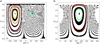 |
Fig. 6 𝓗2(e2, ∆ϖ) contour curves in the 1:1 MMR for a system with m2/m1 = 1 and 𝒜𝓜norm = 0.9. (a) The first projection shows a near planar subsurface with σ ~ 120°. (b) The second projection shows a near planar subsurface with σ ~ 0° .In both panels, the nine numerical integrations are drawn in colors. The red crosses indicate the initial condition in each case. |
Exoplanet elements in system HD 73526 (Wittenmyer et al. 2014), whose host star mass is m0 = 1.014 M⊙.
4.2.2 System HD 31527
System HD 31527 is composed of three exoplanets whose orbital elements are summarized in Table 2. According to Gallardo et al. (2021), planets c and d are in a very uncommon MMR, the 16:3 MMR. In this case, we show the projection of surface 𝓗1 in Fig. 8 since the three-dimensional representation is extremely complex.
This is an interesting case because the secular evolution of the system is really close to the a phase-space separatrix that defines whether the system is in the ACR condition. Currently, e1 = 0.03, but in the future, it way reach values that are higher by one magnitude, regardless of whether it is in the ACR condition (see Fig. A.2).
The secular frequency relation between the orbital elements and the critical angle contrast with the system HD 73526 because in this case, for each secular period of ∆ϖ and the eccentricities, there are seven secular periods of the center of libration. This is closely related to the complexity of the 𝓗 surface (which we do not show).
We clarify that the numerical integration for this system was performed considering planets c and d alone. When we compare them with the numerical integration results shown in Gallardo et al. (2021), who considered planet b, there is a difference in the behaviour of ∆ϖ. Specifically, they obtained that ∆ϖ usually oscillates with some eventual circulations, while we obtained that it circulates in general.
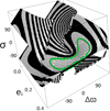 |
Fig. 7 𝓗1 surface compared to a 10 kyr numerical integration (green curve) of the HD 73526 extrasolar system. The orbital elements are listed in Table 1. |
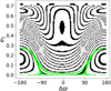 |
Fig. 8 𝓗1 surface projection compared to a 100 kyr numerical integration (green curve) of the HD 31527 extrasolar system. The orbital elements are listed in Table 2. The red cross indicates the initial conditions. |
Exoplanet elements in system HD 31527 (Gallardo et al. 2021), whose host star mass is m0 = 0.96 M⊙.
5 Conclusions
The main conclusion of our work is that we successfully extended the resonant prescription in Gallardo et al. (2021) by applying the method constructed in Pons & Gallardo (2022). In that work, we studied the secular evolution of resonant motions in the framework of an elliptical restricted planar three-body problem. This model allowed us to visualize the phase space in a three-dimensional phase portrait we call 𝓗 surface. This phase portrait provided us with the secular evolution information of e1, e2, ∆ϖ, and σ (or θ). This has several advantages, the most important of which is the capability of encountering exhaustively all the families (or subsurfaces) of resonant evolution that can exist. It is also useful to distinguish a resonant motion with a circulating libration center from a nonresonant motion, where the critical angle circulates on resonant timescales.
We divided the study cases into two groups, the general cases, and the real cases. In the first group, we chose the most common MMRs, which are the 2:1, 3:2, 3:1, and 1:1 MMR. This last MMR, also known as co-orbital motion, is interesting because not every model is capable of describing it. We showed the two most interesting results obtained after exploring several generic systems for each MMR. This uncovered the great complexity that can exist in phase space, and also the high-eccentricity excursions that in some conditions can occur on secular timescales.
We presented two real exoplanet systems in different evolving conditions. First, system HD 73526, which is in an ACRI condition where e1 presents relatively low excursions, but with a moderately high absolute value. This could imply that some other mechanism has excited its eccentricity to such high values, and then, the system encountered a stable condition to continue its evolution.
The other real system we analyzed is system HD 31527, which is in a veryy rare 16:3 MMR and also very close to the strange condition in which it alternates between being in and out of an ACR. In this case, e1 evolves between low and moderate values, whereas e2 remains almost unchanged at a high value.
Because there is no encounter between the planets and they are in a deep MMR condition, the numerical integrations agreed with the model in all cases we studied, which is remarkable. A small correction in initial semi-major axis was sometimes required in order to be in the deep MMR condition. Another important detail that ensured that the deep MMR resonant condition (and therefore, the adiabatic invariant principle) was not broken were the initial conditions for the systems, so that they lay in a closed-contour curve on the 𝓗 surface.
Acknowledgements
The completion of this work was possible not only by the authors’ willingness and determination but also by the support of the CSIC – UdelaR since this was done in the CSIC I+D 2022 “Dinámica Secular y Resonante en Sistemas Planetarios” project context. We also want to mention the valuable corrections and comments given by Jérémy Couturier that help us significantly improve the quality of this article.
Appendix A Mathematical developments
A.1 Canonical transformation
In this section, we outline that the transformation from variables 1 to variables 4 is canonical.
There are several ways to prove whether a given transformation is canonical. We verified this by confirming whether the matrix 𝕄 associated with the transformation satisfied the symplectic condition.
This matrix the Jacobian of the new variables with respect to the old ones. Therefore, it is easy to see that
 (A.1)
(A.1)
In the context of Hamiltonian mechanics, the matrix 𝕄 satisfies the symplectic condition if (Goldstein 1987)
 (A.2)
(A.2)
where 𝕁 is an antisymmetric matrix, defined as follows:
 (A.3)
(A.3)
Here, 𝕆4x4 represents the null matrix, and 𝕀4x4 represents the identity matrix. Both are 4x4 matrices.
Equation A.2 states that the transformation (represented by the matrix 𝕄) preserves the symplectic structure. This means that after the transformation is performed, the canonical Hamil-tonian equations are still valid. For the sake of brevity, we do not show the detailed calculations here that prove the fulfillment of the condition A.2.
A.2 Averaged disturbing function
The third term in equation 2 was averaged to obtain the function 𝓡, the calculation of which was carried out following the approach adopted by Gallardo (2006, 2019, 2020),
 (A.4)
(A.4)
We assumed that during k1 revolutions of the outer planet (and therefore, k2 revolutions of the inner planet), ai, ei, and ∆ϖ remain constant, which is reasonable because the variations in these elements tend to be much more slowly than those of σ (Gallardo et al. 2021). For this calculation, we set a1 to the nominal value given by equation 8. The function R represents the instantaneous disturbing function defined in equation 3.
The relation λ1(λ2, σ) was obtained from Equation 9, which represents the resonant condition2.
A.3 Stable equilibrium points
We demonstrate that stable solutions3 occur at the local minima of the disturbing function. To do this, we followed the idea of small oscillations that was used, for example, in Gallardo (2020).
The idea is to consider small displacements of the equilibrium points on the resonant timescale. Let  be an equilibrium point, that is, values that satisfy the equations 7. We define the small displacements as
  and s = σ − σ0. It is easy to see that
 (A.5)
(A.5)
where in the last equality of each equation, we introduce the compact notation for partial derivatives.
We performed a first-order expansion of the functions 𝓗σ(I1,σ) and  . The result expressed in terms of the variables S and s in matrix form is
 (A.6)
(A.6)
For the equilibrium point  to be stable, the eigenvalues of the matrix in equation A.6 must be purely imaginary. Therefore, we proceeded to calculate the characteristic polynomial of Q,
 (A.7)
(A.7)
The eigenvalues are given by the roots of the characteristic polynomial. We proceeded to compute them and imposed the stability condition
 (A.8)
(A.8)
We recall the expression for the Hamiltonian (Eq. (6)) and have
 (A.9)
(A.9)
Therefore, the only way for λ2 < 0 to hold is if 𝓡σσ > 0. This corresponds to positive concavity in the perturbing function, in other words, the condition for a local minimum. Using this procedure, we can conclude that if 𝓡σσ < 0 (local maximum), then the evolution of that equilibrium point is unstable.
A.4 Time evolution of real exoplanet examples
In this section we report the results of numerical integrations of the two real exoplanet systems in the time domain.
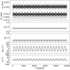 |
Fig. A.1 Orbital element evolution in the time domain for exoplanet system HD 73526. |
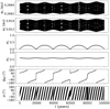 |
Fig. A.2 Orbital element evolution in the time domain for exoplanet system HD 31527. This integration was computed considering only the planets involved in the MMR. σ librates around a long-term circulating libration center. |
References
- Batygin, K., & Morbidelli, A. 2013, A&A, 556, A28 [NASA ADS] [CrossRef] [EDP Sciences] [Google Scholar]
- Beaugé, C., & Michtchenko, T. A. 2003, MNRAS, 341, 760 [Google Scholar]
- Beaugé, C., Ferraz-Mello, S., & Michtchenko, T. A. 2003, ApJ, 593, 1124 [Google Scholar]
- Callegari, N., J., Michtchenko, T. A., & Ferraz-Mello, S. 2004, Celest. Mech. Dyn. Astron., 89, 201 [NASA ADS] [CrossRef] [Google Scholar]
- Chambers, J. E. 1999, MNRAS, 304, 793 [Google Scholar]
- Charalambous, C., Teyssandier, J., & Libert, A. S. 2022, MNRAS, 514, 3844 [NASA ADS] [CrossRef] [Google Scholar]
- Ferraz-Mello, S. 1988, in Long-term Dynamical Behaviour of Natural and Artificial N-body Systems, ed. A. D. Roy, 245 [CrossRef] [Google Scholar]
- Gallardo, T. 2006, Icarus, 184, 29 [Google Scholar]
- Gallardo, T. 2019, Icarus, 317, 121 [NASA ADS] [CrossRef] [Google Scholar]
- Gallardo, T. 2020, Celest. Mech. Dyn. Astron., 132, 9 [Google Scholar]
- Gallardo, T., Beaugé, C., & Giuppone, C. 2021, A&A, 646, A148 [NASA ADS] [CrossRef] [EDP Sciences] [Google Scholar]
- Giuppone, C. A., Beaugé, C., Michtchenko, T. A., & Ferraz-Mello, S. 2010, MNRAS, 407, 390 [NASA ADS] [CrossRef] [Google Scholar]
- Gladman, B. 1993, Icarus, 106, 247 [Google Scholar]
- Goldstein, H. 1987, Mecánica clásica (Reverté) [Google Scholar]
- Haghighipour, N., Couetdic, J., Varadi, F., & Moore, W. B. 2003, ApJ, 596, 1332 [NASA ADS] [CrossRef] [Google Scholar]
- Henrard, J. 1993, The Adiabatic Invariant in Classical Mechanics, eds. C. K. R. T. Jones, U. Kirchgraber, & H. O. Walther (Berlin, Heidelberg: Springer Berlin Heidelberg), 117 [Google Scholar]
- Laskar, J. 1997, A&A, 317, L75 [NASA ADS] [Google Scholar]
- Michtchenko, T. A., Beaugé, C., & Ferraz-Mello, S. 2008, MNRAS, 387, 747 [NASA ADS] [CrossRef] [Google Scholar]
- Petit, A. C., Laskar, J., & Boué, G. 2017, A&A, 607, A35 [NASA ADS] [CrossRef] [EDP Sciences] [Google Scholar]
- Pons, J., & Gallardo, T. 2022, MNRAS, 511, 1153 [NASA ADS] [CrossRef] [Google Scholar]
- Quillen, A. C., & French, R. S. 2014, MNRAS, 445, 3959 [NASA ADS] [CrossRef] [Google Scholar]
- Wittenmyer, R. A., Tan, X., Lee, M. H., et al. 2014, ApJ, 780, 140 [Google Scholar]
- Zhou, L.-Y., Lehto, H. J., Sun, Y.-S., & Zheng, J.-Q. 2004, MNRAS, 350, 1495 [NASA ADS] [CrossRef] [Google Scholar]
Formally, the condition is that σ librates.
In this context, we refer to stable solutions as oscillatory solutions with a constant amplitude.
All Tables
Exoplanet elements in system HD 73526 (Wittenmyer et al. 2014), whose host star mass is m0 = 1.014 M⊙.
Exoplanet elements in system HD 31527 (Gallardo et al. 2021), whose host star mass is m0 = 0.96 M⊙.
All Figures
|
Fig. 1 Averaged resonant Hamiltonian contour curves in plane (a2, σ) in 3:1 MMR for a system with m1 = m2, e1 = 0,47, e2 = 0,38, and ∆ϖ = 84°. |
| In the text | |
|
Fig. 2 Normalized angular momentum function 𝒜𝓜norm(e1, e2) for 2:1 MMR with m2 = m1. (a) Three-dimensional plot of 𝒜𝓜norm(e1, e2). (b) 𝒜𝓜norm(e1, e2) contour curves with numerical values above the curves. |
| In the text | |
|
Fig. 3 Phase portraits for MMR 2:1 and 𝒜𝓜norm = 0.9. (a) 𝓗2 surface for a system with m2/m1 = 0.2. The ten numerical integrations run for 10 kyr are plotted in colors (some areas of the surface were removed for clarity). (b) 𝓗1 surface for a system with m2/m1 = 1. The nine numerical integrations run for 1 kyr are shown. |
| In the text | |
|
Fig. 4 𝓗1 (e1, ∆ϖ) contour curves for the 3:2 MMR for two different systems. (a) First system: m2/m1 = 1 and 𝒜𝓜norm = 0.95. (b) Second system: m2/m1 = 5 and 𝒜𝓜norm = 0.9. In both panels, the numerical integrations are drawn in color. The red crosses indicate the initial condition in each case. |
| In the text | |
|
Fig. 5 Phase portraits for MMR 3:1. (a) 𝓗1 surface for a system with m2/m1 = 1 and 𝒜𝓜norm = 0.8. The ten numerical integrations run for 10 kyr are plotted in colors. (b) 𝓗1 surface for a system with m2/m1 = 0.2 and 𝒜𝓜norm = 0.99. The five numerical integrations run for 1 kyr are shown. |
| In the text | |
|
Fig. 6 𝓗2(e2, ∆ϖ) contour curves in the 1:1 MMR for a system with m2/m1 = 1 and 𝒜𝓜norm = 0.9. (a) The first projection shows a near planar subsurface with σ ~ 120°. (b) The second projection shows a near planar subsurface with σ ~ 0° .In both panels, the nine numerical integrations are drawn in colors. The red crosses indicate the initial condition in each case. |
| In the text | |
|
Fig. 7 𝓗1 surface compared to a 10 kyr numerical integration (green curve) of the HD 73526 extrasolar system. The orbital elements are listed in Table 1. |
| In the text | |
|
Fig. 8 𝓗1 surface projection compared to a 100 kyr numerical integration (green curve) of the HD 31527 extrasolar system. The orbital elements are listed in Table 2. The red cross indicates the initial conditions. |
| In the text | |
|
Fig. A.1 Orbital element evolution in the time domain for exoplanet system HD 73526. |
| In the text | |
|
Fig. A.2 Orbital element evolution in the time domain for exoplanet system HD 31527. This integration was computed considering only the planets involved in the MMR. σ librates around a long-term circulating libration center. |
| In the text | |
Current usage metrics show cumulative count of Article Views (full-text article views including HTML views, PDF and ePub downloads, according to the available data) and Abstracts Views on Vision4Press platform.
Data correspond to usage on the plateform after 2015. The current usage metrics is available 48-96 hours after online publication and is updated daily on week days.
Initial download of the metrics may take a while.