| Issue |
A&A
Volume 681, January 2024
|
|
|---|---|---|
| Article Number | A34 | |
| Number of page(s) | 9 | |
| Section | Astrophysical processes | |
| DOI | https://doi.org/10.1051/0004-6361/202347258 | |
| Published online | 05 January 2024 | |
Dissecting the emission from LHAASO J0341+5258: Implications for future multiwavelength observations
1
Astronomy & Astrophysics Group, Raman Research Institute, C. V. Raman Avenue, 5th Cross Road, Sadashivanagar, Bengaluru, 560080 Karnataka, India
e-mail: agnibha@rri.res.in
2
Saha Institute of Nuclear Physics, A CI of Homi Bhabha National Institute, Kolkata, 700064 West Bengal, India
Received:
22
June
2023
Accepted:
7
September
2023
Context. The Large High Altitude Air Shower Observatory (LHAASO) has detected multiple ultra-high-energy (UHE; Eγ ≥ 100 TeV) gamma-ray sources in the Milky Way Galaxy, which are associated with Galactic “PeVatrons” that accelerate particles up to PeV (=1015 eV) energies. Although supernova remnants (SNRs) and pulsar wind nebulae (PWNe), as source classes, are considered the leading candidates, further theoretical and observational efforts are needed to find conclusive proof that can confirm the nature of these PeVatrons.
Aims. The aim of this work is to provide a phenomenological model to account for the emission observed from the direction of LHAASO J0341+5258, an unidentified UHE gamma-ray source observed by LHAASO. Further, we also aim to provide the implications of our model in order to support future observations at multiple wavelengths.
Methods. We analyzed 15 yr of Fermi-LAT data to find the high-energy (HE; 100 MeV ≤ Eγ ≤ 100 GeV) GeV gamma-ray counterpart of LHAASO J0341+5258 in the 4FGL-DR3 catalog. We explain the spectrum of the closest 4FGL source, 4FGL J0340.4+5302, by a synchro-curvature emission formalism. We explored the escape-limited hadronic interaction between protons accelerated in an old, now invisible SNR and cold protons inside associated molecular clouds (MCs) and leptonic emission from a putative TeV halo in an effort to explain the multiwavelength (MWL) spectral energy distribution (SED) observed from the LHAASO source region.
Results. The spectrum of 4FGL J0340.4+5302 is explained well by the synchro-curvature emission, which, along with its point-like nature, indicates that this object is likely a GeV pulsar. A combined lepto-hadronic emission from SNR+MC and TeV halo scenarios explains the MWL SED of the LHAASO source. In addition, we find that leptonic emission from an individual TeV halo is also consistent with the observed MWL emission. We discuss possible observational avenues that can be explored in the near future and predict the outcome of those observational efforts from the model explored in this paper.
Key words: radiation mechanisms: non-thermal / pulsars: general / gamma rays: general / ISM: supernova remnants
© The Authors 2024
 Open Access article, published by EDP Sciences, under the terms of the Creative Commons Attribution License (https://creativecommons.org/licenses/by/4.0), which permits unrestricted use, distribution, and reproduction in any medium, provided the original work is properly cited.
This article is published in open access under the Subscribe to Open model. Subscribe to A&A to support open access publication.
1. Introduction
The nature and emission mechanism of Galactic PeVatrons have become a matter of intense debate after the detection of more than a dozen ultra-high-energy (UHE) gamma-ray sources in the Milky Way Galaxy by LHAASO (Cao et al. 2021a) since it became operational in 2020 April (Cao 2010). In addition, successful operations by Tibet-ASγ and the High-Altitude Water Cherenkov (HAWC) have ushered in the era of UHE gamma-ray astronomy (Abeysekara et al. 2020; Amenomori et al. 2019). Although most of these sources are unidentified, it has been proposed that both supernova remnants (SNRs) associated with dense molecular clouds (MCs), that is SNR+MC systems, and pulsar wind nebulae (PWNe)/TeV halo systems have the necessary energetics to be the PeVatrons associated with UHE gamma-ray sources. After Crab PWN was confirmed to be a PeVatron (Cao et al. 2021b), the PWN interpretation of PeVatrons began to be heavily favored. However, recent efforts have suggested that even if a powerful pulsar is present in the vicinity of a UHE gamma-ray source, it is not guaranteed that the corresponding PWN is a PeVatron (De Sarkar et al. 2022b). Furthermore, detailed studies also dictated that SNRs associated with dense MCs are viable candidates for being PeVatrons (De Sarkar & Gupta 2022; De Sarkar 2023; Abe et al. 2023). Future observational studies by the Cherenkov Telescope Array (CTA; Cherenkov Telescope Array Consortium 2019) and the Southern Wide-field Gamma-ray Observatory (SWGO; Albert et al. 2019) will be crucial in confirming the nature and emission of PeVatrons.
In this paper, we provide a phenomenological model to explain the MWL emission from the direction of an unidentified UHE gamma-ray source, LHAASO J0341+5258, reported by Cao et al. (2021c). This source was detected at the best-fit position of right ascension (RA) = 55.34° ± 0.11°, and declination (Dec) = 52.97° ± 0.07°, with a significance of 8.2σ above 25 TeV. Cao et al. (2021c) reported that the LHAASO source is spatially extended, where the extension of the source was estimated to be σext = 0.29° ±0.06°, with a TSext (≡2 log(ℒext/ℒPS)) of ∼13. No apparent energetic pulsar or SNR was found near the LHAASO source. However, using multiline CO observations (12CO and 13CO) of the region performed as part of the Milky Way Imaging Scroll Painting (MWISP) project (Su et al. 2019), dense MCs were found to partially overlap with the LHAASO source. Previously, scenarios including leptonic emission from pulsar halo (Cao et al. 2021c), hadronic interaction between SNR and MCs (Cao et al. 2021c), and injection of particles from past explosions (Kar & Gupta 2022) were explored, but none of these models explained the MWL SED entirely. Our simple model is designed to provide a feasible MWL emission mechanism to explain the observed MWL SED associated with LHAASO J0341+5258, while accounting for the disappearance of a possible SNR at the present day. We also aim to explain the presence of a TeV halo associated with a putative, energetic GeV pulsar within the LHAASO source extent.
In Sect. 2, we discuss the results obtained from this work. In Sect. 2.1, we present the results of a Fermi-LAT data analysis of the probable GeV counterpart of the LHAASO source, 4FGL J0340.4+5302. In Sect. 2.2, we then provide the basic formalism of the synchro-curvature radiation that has been used to explain the spectrum of the 4FGL source. In Sects. 2.3 and 2.4, the models considering the hadronic interaction in the SNR+MC system and the leptonic interaction in the putative TeV halo are discussed, respectively. Finally, we discuss overall results of our study in Sect. 3, and provide conclusions in Sect. 4.
2. Results
2.1. Fermi-LAT data analysis
We analyzed 15 yr (2008 August 4–2023 May 1) of PASS 8 Fermi-LAT data in the energy range of 0.1–500 GeV using Fermipy1 version 1.2.0 (Wood et al. 2017). To avoid contamination from the Earth’s albedo gamma rays, the events with a zenith angle of greater than 90° were excluded from the analysis. The instrument response function, Galactic diffuse emission template (galdiff), and isotropic diffuse emission template (isodiff) used in this analysis are “P8R3_SOURCE_V3”, “gll_iem_v07.fits”, and “iso_P8R3_SOURCE_V3_v1.txt”, respectively. We used the latest 4FGL catalog, 4FGL-DR3, to study the GeV counterpart of LHAASO J0341+5258 (Abdollahi et al. 2022).
We considered a circular region of interest (ROI) with a radius of 20°, of which the center coincides with the centroid of the LHAASO source, in order to extract the data from the Fermi-LAT website2. Within that ROI, we considered a rectangular region of 15° ×15° positioned at the centroid of the LHAASO source. Galdiff, isodiff, and all of the 4FGL sources within that rectangular region were included in the data analysis. The normalization parameters of the 4FGL sources, within 5° angular extent of the LHAASO source centroid, including all of the parameters of galdiff and isodiff, were kept free during the data analysis. Previously undetected point sources in the vicinity of the LHAASO source, with a minimum TS value of 25 and a minimum separation of 0.3° between any two point sources, were explored using the source-finding algorithm of Fermipy. However, no plausible point sources relevant to this case were found in the spatial proximity of the LHAASO source. A maximum-likelihood analysis was performed to ascertain the best-fit values of the spatial and spectral parameters of the relevant 4FGL sources, as well as those of galdiff and isodiff. With the exception of 4FGL J0340.4+5302, which is the probable GeV counterpart of the LHAASO source, the other 4FGL sources, as well as galdiff and isodiff, were considered as background and were therefore subtracted during the analysis. The data analysis procedure discussed above is similar to that followed in De Sarkar et al. (2022a).
Cao et al. (2021c) analyzed 4FGL-DR2 data and found the same GeV counterpart 4FGL J0340.4+5302 within the extension of LHAASO J0341+5258. We rechecked the properties of the 4FGL source with updated 4FGL-DR3 data to ascertain the localization, extension, and spectrum of the source. The 4FGL source was located at RA = 55.135° ± 0.013° and Dec = 53.083° ± 0.011° with a significance of 64.61σ, 0.154° away from the centoid of the LHAASO source. Similarly to Cao et al. (2021c), we found the spectrum of the 4FGL source to be significantly curved (TScurve ≡ 2 log(ℒLP/ℒPL) ∼ 325.74) and well-fitted by a log-Parabola spectrum, that is, dN/dE ∝ (E/Eb)−αLP − βLP log(E/Eb), with best-fit spectral parameters of αLP = 3.106 ± 0.047, βLP = 0.483 ± 0.033, and Eb = 0.541 GeV, and a corresponding energy flux of ∼5.447 × 10⁻¹¹ erg cm−2 s−1 in the energy range of 0.1–500 GeV. The source extension was checked with a RadialDisk model. The 95% confidence level upper limit of the extension of the 4FGL source was found to be σdisk ≤ 0.29°, with TSext of ∼15.08 (3.88σ), indicating that the 4FGL source is a point-like source. Due to the point-like extension and the curved spectral signature associated with the 4FGL source, we propose that 4FGL J0340.4+5302 is possibly a pulsar emitting in the GeV gamma-ray range, which agrees with the conclusions of Cao et al. (2021c).
2.2. Synchro-curvature emission from a putative pulsar
To test the GeV pulsar interpretation of the 4FGL source, we explored the synchro-curvature emission formalism, which was previously used to explain GeV gamma-ray emission from pulsars (Cheng & Zhang 1996; Kelner et al. 2015). The GeV gamma-ray emission from energetic pulsars has been conventionally explained by two general mechanisms: (a) curvature emission, where the radiation is produced by relativistic electron–positron pairs streaming along the curved magnetic field lines with a radius of curvature, and (b) synchrotron emission, where the radiation is produced by the same pairs gyrating around a straight magnetic field line. Although both of these emission mechanisms explain the GeV gamma-ray emission from pulsars well, in a realistic scenario, it can be clearly understood that the relativistic charged particles streaming along the curved magnetic field lines must also spiral around them. Consequently, rather than proceeding in either the curvature or the synchrotron radiation modes, an intermediate emission scenario termed the synchro-curvature radiation, should be considered the general radiation mechanism responsible for the gamma rays observed from GeV pulsars (for further details, see Cheng & Zhang 1996; Viganò et al. 2015a). Hence, in this work, we try to explain the spectrum of the 4FGL source with the synchro-curvature process, which is assumed to take place in the outer gap of the pulsar magnetosphere. In this section, we outline the governing equations relevant to the synchro-curvature radiation formalism. For a detailed discussion on the topic, we refer readers to Cheng & Zhang (1996), Viganò & Torres (2015), Viganò et al. (2015a,b).
The particles spiraling around a curved magnetic field with a radius of curvature rc and magnetic field B emit photons with a characteristic energy of
where Γ is the relativistic Lorentz factor, α is the pitch angle (angle between B and v), and ℏ (≈1.0546 × 10⁻²⁷ cm2 g s−2 K−1) is the reduced Planck’s constant. The gyro-radius (or Larmor radius) rgyr and the factor Q2 are given by
![$$ \begin{aligned}&Q_2^2 = \frac{\cos ^4 \alpha }{r_{\rm c}^2}\left[1 + 3\xi + \xi ^2 + \frac{r_{\rm gyr}}{r_{\rm c}} \right], \end{aligned} $$](/articles/aa/full_html/2024/01/aa47258-23/aa47258-23-eq3.gif)
where me is the electron rest mass, and c is the velocity of light. The synchro-curvature parameter ξ is given by
The power radiated by a single particle per unit energy at a given position is given by
![$$ \begin{aligned} \frac{\mathrm{d} P_{\rm sc}}{\mathrm{d} E} = \frac{\sqrt{3} e^2 \Gamma { y}}{4 \pi \hbar r_{\rm eff}}\left[(1+z)F({ y}) - (1-z)K_{2/3}({ y}) \right], \end{aligned} $$](/articles/aa/full_html/2024/01/aa47258-23/aa47258-23-eq5.gif)
where
where E is the photon energy, Kn are the modified Bessel functions of the second kind of index n, and the effective radius is given by
By integrating Eq. (5) in energy, we get the total synchro-curvature power radiated by a single particle:
where the synchro-curvature correction factor gr is given by
![$$ \begin{aligned} g_{\rm r} = \frac{r_{\rm c}^2}{r_{\rm eff}^2} \frac{\left[1 + 7(r_{\rm eff} Q_2)^{-2}\right]}{8 (Q_2 r_{\rm eff})^{-1}}\cdot \end{aligned} $$](/articles/aa/full_html/2024/01/aa47258-23/aa47258-23-eq11.gif)
We further obtained the details of the trajectories of the charged particles by numerically solving their equations of motion:
In this equation, the relativistic momentum (with the velocity assumed to be constant at v = c) of the charged particles, p (= ), is directed toward
  , and the constant accelerating electric field, E||, is directed toward
  , that is, tangential to the curved magnetic field lines. Breaking down the equations of motion into parallel (p|| = p cos α) and perpendicular (p⊥ = p sin α) components, we get
Equations (13) and (14) are numerically solved to determine the evolution of the Lorentz factor Γ, sin α, and synchro-curvature parameter ξ along the trajectory of motion.
Similar to Viganò et al. (2015a), we calculate the average synchro-curvature radiation spectrum throughout the trajectory using the equation
where the integration limits have been chosen to be the distance depicting the injection point of the particles (x = 0), and the maximum distance up to which the spectrum can be emitted (x = xmax). Furthermore, the effective weighted particle distribution function, which takes into account the depletion of the number of emitting particles directed toward the observer at a distance x from their injection point, is given by the following equation (Viganò et al. 2015a):
where N0, the normalization of the effective particle distribution, is such that  , and x0 is the length scale of the same.
The model discussed above is based on the dynamics of relativistic lepton pairs that move along curved magnetic field lines in an acceleration region of the pulsar magnetosphere. We performed this calculation whilst considering three free parameters:
-
The electric field parallel to the magnetic field, E|| (V m−1), which is assumed to be constant throughout the acceleration region. We varied this parameter within the range log(E|| (V m−1)) = 6.5–9.5 (Viganò & Torres 2015). The accelerating electric field explains the energy peak of the synchro-curvature spectrum.
-
The length scale, x0/rc, which depicts the spatial extent of the emitting region for injected particles. We varied this parameter within the range x0/rc = 0.001 − 1 (Viganò & Torres 2015). The variation of this parameter determines the low-energy slope of the spectrum.
-
The overall normalization parameter, N0, which depicts the total number of charged particles in the acceleration region, whose radiation is directed toward the observer. The overall normalization N0 has been varied to explain the spectrum of the 4FGL source. We varied this parameter within the range of N0 = 1026–1034 particles (Viganò & Torres 2015).
The remaining parameters are considered to be fixed following Viganò et al. (2015a), that is, magnetic field B = 106 G, radius of curvature rc = 108 cm, and maximum distance of the emitting region xmax = rc = 108 cm. Two coupled ordinary differential equations, Eqs. (13) and (14), are numerically solved simultaneously to evaluate the evolution of the Lorentz factor Γ, the pitch angle in terms of sin α, and the synchro-curvature parameter ξ. To solve these equations, we typically set the initial values for the Lorentz factor and the pitch angle to Γin = 103 and αin = 45° (Viganò et al. 2015a). We note that although the magnetic field can be ideally parameterized as a function of the timing properties and the magnetic gradient (Viganò & Torres 2015; Viganò et al. 2015b), because of our lack of knowledge regarding those parameters in this case, we consider the magnetic field to be constant at a value consistent with that explored by Viganò et al. (2015a).
Figure 1 shows the evolution of the Lorentz factor Γ (panel a), the pitch angle α (panel b), and the synchro-curvature parameter ξ (panel c), as well as the model spectrum plotted against the SED data points of the 4FGL source (panel d). The values of the free parameters considered in this model to explain the SED of 4FGL J0340.4+5302 are log(E|| (V m−1)) = 7.113, x0/rc = 0.15, and N0 = 1.3 × 1031 particles, where the distance to the pulsar was assumed to be 1 kpc (Cao et al. 2021c). From panel d of Fig. 1, it can be seen that the synchro-curvature emission model explains the SED of the 4FGL source quite well, which in turn indicates that 4FGL J0340.4+5302 indeed shows spectral features typical of a GeV pulsar. Detection of pulsed emission from this source in radio and gamma rays would confirm its nature in the future.
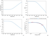 |
Fig. 1. Outputs of the synchro-curvature model. Here, we show the evolution of (a) Lorentz factor Γ, (b) pitch angle α, and (c) synchro-curvature parameter ξ. In panel d, the model spectrum is plotted against the SED data points obtained from Fermi-LAT analysis of 4FGL J0340.4+5302. |
2.3. Emission from the SNR+MC association
In this section, we discuss the full model and the relevant parameters of the hadronic interaction model, in which gamma rays are produced from the inelastic p–p interaction between protons accelerated in the shock front of an old, now invisible shell-type SNR and the cold protons residing in the MCs surrounding the SNR. We used the open-source code GAMERA3 (Hahn 2016) to calculate the gamma-ray SED from the hadronic p–p interaction. For a detailed discussion on the formalism, we refer readers to De Sarkar & Gupta (2022), De Sarkar (2023), Fujita et al. (2009), Ohira et al. (2010), and Makino et al. (2019).
The model assumes that a supernova (SN) explosion occurred inside a tenuous, spherical cavity surrounded by dense MCs. After the explosion, following the initial free-expansion phase, the SNR enters the adiabatic Sedov-Taylor phase, during which the time evolution of the shock velocity and shock radius is given by the following relations (De Sarkar & Gupta 2022; Fujita et al. 2009):
and
where we assume an initial shock velocity of vi = 109 cm s−1, and an SNR age and radius at the onset of the Sedov phase of tSedov ≈ 210 yr and RSedov ≈ 2.1 pc, respectively. The cosmic ray (CR) protons are accelerated through diffusive shock acceleration (DSA) at the shock front. We adopt an escape-limited scenario of proton acceleration (Ohira et al. 2010), where these accelerated protons need to escape a geometrical confinement region around the shock front – produced by strong magnetic turbulence – in order to participate in gamma-ray production after the shock front collides with the surrounding MCs. The distance of the outer boundary of this confinement region (escape boundary) from the center of the cavity, that is, the escape radius, is given by

where κ (≈0.04) is defined by the relation lesc = κRsh, where lesc is the radial distance of the escape boundary from the shock front (Ohira et al. 2010; Makino et al. 2019).
It has previously been assumed that the acceleration of protons stops at the time of collision t = tcoll, which is when the escape radius is equal to the distance of the MC surface from the cavity center (i.e., Resc(tcoll)≈Rsh(tcoll) = RMC) (Fujita et al. 2009). Therefore, only the protons that have been accelerated before the collision and possess sufficient energy to escape the escape boundary will take part in producing UHE gamma rays. This threshold energy of proton escape can be given by the phenomenological relation (Makino et al. 2019; Ohira et al. 2012)
where αSNR signifies the evolution of the escape energy during the Sedov phase (Makino et al. 2019). We note that in this case, it has been assumed that the protons get accelerated up to a maximum energy of  eV (knee energy) at the onset of the Sedov phase (Gabici et al. 2009). We consider αSNR as a free parameter, and
  , where
  is the minimum energy of the escaped proton population. The spectrum of the escaped proton population is given by the following equation (Ohira et al. 2010):
![$$ \begin{aligned} N_{\rm esc}(E_{\rm p}) \propto E_{\rm p}^{-[s + (\beta /\alpha _{\rm SNR})]} \propto E_{\rm p}^{-p_{\rm SNR}}, \end{aligned} $$](/articles/aa/full_html/2024/01/aa47258-23/aa47258-23-eq28.gif)
where β = 3(3–s)/2 (Makino et al. 2019), assuming the thermal leakage model of CR injection (Ohira et al. 2010). For s = 2, as is expected from DSA, we find β = 1.5. We note that the minimum energy (Eq. (20)) and the spectral shape (Eq. (21)) of the escaped proton population, as well as the gamma-ray production from the hadronic p–p interaction (Kafexhiu et al. 2014), are all estimated at the collision time t = tcoll. In the present work, we phenomenologically varied the value of the free parameter αSNR and chose this to be αSNR = 1.5. Considering the chosen value of αSNR, our model indicates that the expanding SNR shock collided with the surrounding dense MCs at an age of tcoll ∼ 6.1 × 10³ yr. At time t = tcoll, the radius and the velocity of the SNR shock front were found to be Rsh(tcoll)∼20.27 pc (which is also equal to RMC at the time of collision), and vsh(tcoll)∼1.3 × 108 cm s−1, respectively. Following the collision, the escaped proton population – accelerated until the collision epoch – enters the MC medium to produce gamma rays through hadronic p–p interactions. The minimum energy of this escaped proton population is found to be  TeV, calculated using Eq. (20) for the choice of the parameter αSNR, whereas, as discussed above, the maximum energy is given by
  TeV. Furthermore, using values of s, β, and αSNR, we calculate a spectral index of pSNR = 3.0 for the escaped proton population, and the corresponding spectral shape was given by Eq. (21). We find the total energy budget of the escaped proton population required to explain the gamma-ray SED to be WSNR ∼ 1.7 × 1046 erg, where the number density inside the MC medium and the SNR+MC source distance are assumed to be nMC ∼ 50 cm−3 and d = 1 kpc, respectively, following Cao et al. (2021c).
At t = tcoll, the shock can be assumed as a shell with a radius of Rsh(tcoll) (=RMC) centered at the cavity. At t > tcoll, the shock enters the momentum-conserving, snow-plow phase and continues to expand inside the MC medium. If the radius of the shell inside the MC medium is Rshell, then its time evolution inside the MCs can be estimated by solving the momentum conservation equation (Fujita et al. 2009; De Sarkar & Gupta 2022):
![$$ \begin{aligned}&\frac{4\pi }{3}\left[n_{\rm MC} (R_{\rm shell}(t)^3 - R_{\rm sh}(t_{\rm coll})^3) + n_{\rm cav}R_{\rm sh}(t_{\rm coll})^3\right]\dot{R}_{\rm shell}(t)\nonumber \\&{=}~\frac{4\pi }{3}n_{\rm cav}R_{\rm sh}(t_{\rm coll})^3 v_{\rm sh}(t_{\rm coll}), \end{aligned} $$](/articles/aa/full_html/2024/01/aa47258-23/aa47258-23-eq31.gif)
with Rshell = RMC at t = tcoll, and with ncav (≈1 cm−3) being the number density inside the cavity. We note that the velocity of the shocked shell inside the MC medium continues to decrease as it continues to expand with time. As a result, if the SNR shocked shell at the current epoch is sufficiently old, its velocity inside the MCs will definitely be comparatively smaller than the internal gas velocity of the MCs. Consequently, the shocked shell inside the MCs will not be detectable as the remains of the shell will become invisible. We use this fact to explain the nondetection of the possible old SNR and to propose a probable current age of the SNR as well. This approach was used to explain the nondetection of the SNR shell in the case of LHAASO J2108+5157 (De Sarkar 2023). We calculate the time evolution of the SNR shocked shell inside the associated MCs using Eq. (22), and find that the SNR, with a final radius of Rsh(tage)∼32.4 pc, has to be tage ∼ 6.2 × 10⁵ yr old for the shock velocity (vsh(tage)∼8 × 105 cm s−1) to be lower than the internal gas velocity of MCs (∼106 cm s−1; Cao et al. 2021c) and for the SNR shell to disappear. The time evolution of the shocked shell is shown in Fig. 2. Please note that we do not consider the total gamma-ray flux produced from the escaped protons when the shock front is within the MC medium, even if the SNR is still in the Sedov phase. The acceleration and escape of protons will depend on the evolution of the confinement region inside the turbulent MC medium, which is poorly understood. Consequently, we have avoided this contribution altogether so as not to complicate our model, as this contribution is expected to be negligible anyway. Moreover, given the low shock velocity, the full ionization of the pre-shock gas does not occur, making the particle acceleration ineffective when the SNR enters the radiative phase. As a result, the corresponding gamma-ray contribution during the radiative phase of the SNR continues to remain insignificant (see De Sarkar 2023, and references therein). We further note that proton diffusion inside the MC medium has been neglected in this model. The average diffusion coefficient inside the dense, strongly turbulent MC medium (≈1025–1026 cm2 s−1; Gabici et al. 2009) is significantly smaller than that measured in the interstellar medium (≈1028 − 1029 cm2 s−1; De Sarkar et al. 2021). The details regarding the suppressed diffusion inside the MCs are uncertain (Dogiel et al. 2015; Xu et al. 2016), and so we exclude this aspect in order to avoid introducing complications in the simple model discussed in this paper. A similar assumption was also considered in the case of LHAASO J1908+0621 (De Sarkar & Gupta 2022) and for LHAASO J2108+5157 (De Sarkar 2023).
 |
Fig. 2. Time evolution of the shocked shell associated with the old SNR inside the surrounding MCs. |
We note that neutrino emission is considered to be evidence of hadronic interaction in any astrophysical source. Therefore, in order to confirm the presence of a hadronic emission mechanism in this particular source, we compared the total neutrino flux expected from hadronic interaction to the sensitivity of the next-generation IceCube-Gen2 neutrino observatory (Aartsen et al. 2021). We find that the neutrino flux is not significant enough to be detected by IceCube-Gen2. We plot the scaled neutrino flux along with IceCube-Gen2 sensitivity in Fig. 3.
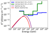 |
Fig. 3. Expected neutrino flux (scaled) against the IceCube-Gen2 sensitivity for two declinations. |
2.4. Emission from the TeV halo
As an energetic pulsar spins down, a wind nebula is created due to the conversion of rotational energy to wind energy, known as the pulsar wind nebula (PWN; Gaensler & Slane 2006). Electron–positron pairs accelerated to ultra-relativistic energies at the termination shock of the wind produce MWL emission because of their interaction with the ambient magnetic field, matter, and radiation fields. As a result, over the years, multiple PWNe have been detected, especially in radio, X-ray, and gamma-ray energy ranges (Gaensler & Slane 2006), and PWNe are considered to be one of the leading candidates for being Galactic PeVatrons (de Oña Wilhelmi et al. 2022). The size of the PWNe can be of the order of 0.1–10 pc, and the associated nebular magnetic field can be estimated to be of the order of 10–1000 μG. PWN is a dynamic source class, which goes through multiple stages of evolution (Giacinti et al. 2020). In the first stage (t < 10 kyr), PWNe can be considered as spherically symmetric systems, in which high-energy leptons are confined by a large magnetic field, and TeV gamma rays are emitted by these leptons. The forward shock of the host SNR expands in the surrounding interstellar medium (ISM), whereas the newly formed reverse shock starts to contract, but does not yet reach the PWN. In the second stage (t = 10–100 kyr), the PWN morphology becomes highly irregular, as at this stage the reverse shock has hit the PWN, thus disrupting it. At this stage, the high-energy leptons escape and propagate inside the surrounding SNR, but not yet in the ISM. In the final stage (t > 100 kyr), the nebula completely disrupts and the host SNR fades away. The high-energy leptons therefore escape into the surrounding ISM, and then slowly diffuse in the strongly turbulent interstellar magnetic field and emit TeV gamma rays in a volume that is much larger than that of the initial PWN.
This extended source class – associated with energetic pulsars – emitting very-high-energy (VHE; 100 GeV ≤ Eγ ≤ 100 TeV) gamma rays, collectively known as the TeV halo, was recently established. These sources shine bright in TeV energies and have a hard spectrum (having an electron injection spectral index of between ∼1.5 and 2.2; Sudoh et al. 2019). TeV halos were first detected by the MILAGRO and HAWC observations of Geminga and PSR B0656+14, where extended TeV gamma-ray emission was discovered surrounding these pulsars from the surface brightness distributions (Abdo et al. 2009; Abeysekara et al. 2017a,b). TeV halos are characterized by a slow diffusion region (e.g., D(Ee) = 4.5 × 1027 (Ee/100 TeV)1/3 cm2 s−1, i.e., 2–3 orders of magnitude smaller than the typical diffusion coefficient of the ISM), with a large spatial extent (rhalo ≈ 20 − 50 pc) (Abeysekara et al. 2017a; Liu 2022). Self-generated CR turbulence or Alfvén waves are popularly considered to be the origin of the slow isotropic diffusion, where a large density gradient of escaped electron–positron pairs near the source induces the growth of small-scale magnetohydrodynamic (MHD) turbulence of the background plasma, otherwise known as the resonant streaming instability. Escaped pairs get trapped by the increased MHD turbulence, which translates into the suppression of the diffusion coefficient. For a comprehensive review, we refer readers to Fang (2022), Liu (2022), and references therein. Separately, multiple models have been proposed to explain the possible origin of TeV halos; namely isotropic, unsuppressed diffusion with the transition from quasi-ballistic propagation (Prosekin et al. 2015), anisotropic diffusion (Liu et al. 2019b), and so on. Further details regarding the origin of the TeV halo are beyond the scope of this paper. Additionally, the magnetic field associated with the TeV halo was also estimated to be at the same level as the average Galactic magnetic field (Sudoh et al. 2019), which is relatively low compared to that observed in PWNe. From X-ray observations, the magnetic field inside the TeV halo of Geminga was constrained to be < 1 μG (Liu et al. 2019a). Therefore, a low estimated magnetic field can also be an important differentiator between the TeV halo and PWN scenarios.
The presence of a putative GeV pulsar 4FGL J0340.4+5302 co-spatial with the LHAASO source region, and the spatially extended gamma-ray emission observed by LHAASO, together suggest the existence of an extended TeV halo emission in the source region. Although it is difficult to ascertain because of the lack of proper distance estimation, in this work, we assume that the putative pulsar 4FGL J0340.4+5302 is associated with the old, invisible SNR, which means that the age of the pulsar is ∼6.2 × 10⁵ yr. From the nondetection of the old SNR and the offset between the LHAASO source centroid and the 4FGL source, it can be posited that the system is old enough to be in the final stage of evolution, where the host SNR has faded away and the corresponding pulsar has been displaced from its original position because of its natal kick velocity (Gaensler & Slane 2006), which makes the TeV halo scenario more plausible.
Consequently, we considered a steady-state relativistic electron population from a putative TeV halo associated with the GeV pulsar and calculated the total leptonic contribution from this source to help explain the MWL SED of the LHAASO source. As a result of slow diffusion inside the TeV halo region, radiative cooling timescales of Ee > 10 TeV leptons that produce TeV gamma rays – that is, ∼104(B/10 μG)−2 (Ee/10 TeV)−1 yr (Giacinti et al. 2020) – are comparatively lower than the escape timescale, which is  yr (Liu 2022). We therefore neglect the effect of lepton escape from the TeV halo source. In a radiation-dominated environment, the inverse-Compton (IC) emission from the accelerated leptons – with a hard spectrum – that escape from the disrupted PWN into the TeV halo can provide a significant contribution to the VHE-UHE gamma-ray regime (Breuhaus et al. 2021). We considered different leptonic cooling mechanisms, such as IC and synchrotron (Baring et al. 1999; Ghisellini et al. 1988; Blumenthal & Gould 1970), to obtain the MWL emission from the parent electron population associated with the TeV halo using GAMERA (Hahn 2016). The synchrotron emission, which is constrained by the X-ray upper limit, should also provide a constraint on the value of the associated magnetic field, which would in turn confirm the TeV halo interpretation of the observed VHE-UHE gamma-ray emission.
To explain the MWL SED of LHAASO J0341+5258, in the present study, we considered two scenarios: (a) a two-zone Lepto-hadronic scenario, where TeV halo emission is used in conjunction with the hadronic emission from the SNR+MC association (see discussion in Sect. 2.3), and (b) a one-zone Leptonic scenario, in which the entire emission is explained by an individual TeV halo, without the presence of any SNR+MC association. We considered the distance of the TeV halo in both cases to be d = 1 kpc. The spectrum of the electron population was assumed to be a simple power law with an exponential cutoff in the form of  exp(
exp( ) for the Lepto-hadronic case, and
  exp(
exp( ) for the Leptonic case. In this case,
  and
and  depict the maximum energy beyond which the rollover in the spectrum ensues. These can also be portrayed as the rollover energy or the cutoff energy of the spectrum. The minimum energy of the electron population was given by the rest-mass energy. We also considered interstellar radiation field following Popescu et al. (2017), and the associated magnetic field in the two cases was fixed by remaining consistent with the X-ray upper limits reported by Cao et al. (2021c).
In both cases, the spectral index of the lepton population was fixed at pLH = pL = 1.5 (Sudoh et al. 2019). For the Lepto-hadronic case, the maximum energy and the energy budget required to explain the MWL SED are  TeV and WLH ∼ 1.5 × 1045 erg, whereas for the Leptonic case these were found to be
  TeV and WL ∼ 1.7 × 1045 erg. The maximum energy estimates in both cases are consistent with the TeV halo scenario, where electrons – with maximum energy ranging from tens to hundreds of TeVs – can be present in the halo region (Liu 2022). The associated magnetic fields, which are constrained by the X-ray upper limits, were estimated to be BLH ≈ 4 μG for the Lepto-hadronic case, and BL ≈ 2.6 μG for the Leptonic case. In both cases, the values of the estimated magnetic fields are well below that typically observed in a standard PWN and are similar to the average value of the Galactic magnetic field in the ISM (2–6 μG), which corroborates the TeV halo interpretation of gamma-ray emission. The model spectrum for (a) Lepto-hadronic and (b) Leptonic cases, along with the data points for the MWL SED of LHAASO 0341+5258 taken from Cao et al. (2021c), are shown in panels a and b of Fig. 4, respectively. As can be seen from the figures, both cases are consistent with the MWL SED and the upper limits obtained up until now.
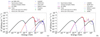 |
Fig. 4. MWL data points, along with the MWL spectra obtained from the two models discussed in this paper, are provided. The (a) Lepto-hadronic model spectrum from combined SNR+MC and TeV halo scenarios, and (b) Leptonic model spectrum from a single TeV halo scenario are plotted against the MWL SED of LHAASO J0341+5258. |
3. Discussion
In this section, we discuss the main implications of the present work in detail. As both the Lepto-hadronic and Leptonic models explain the MWL SED of the LHAASO source, it is difficult to distinguish whether the SNR+MC association or the TeV halo is responsible for the UHE gamma-ray emission observed by LHAASO. Because of the poor angular resolution capability, LHAASO cannot discern the associated PeVatron in the source region. Consequently, VHE gamma-ray observations are required to properly confirm the source contribution from the study of spatial morphology. From Fig. 4, it can be seen that the model spectrum in both cases exceeds the sensitivities of VHE gamma-ray observatories such as CTA north (Cherenkov Telescope Array Consortium 2019), SWGO (Albert et al. 2019), and ASTRI (Vercellone 2023). Therefore, VHE gamma-ray data obtained by these observatories would be crucial to unveiling the nature of the PeVatron and confirming which of these two cases is valid. For example, if the entire emission is due to the leptonic component from a TeV halo, then only a singular emission peak should be observed. On the other hand, if the Lepto-hadronic case is valid, then a double-peaked significance map should be observed in the source region, as it was observed in the case of LHAASO J1908+0621 (De Sarkar & Gupta 2022; Li et al. 2021). Hence, from the study of the spatial morphology using VHE gamma-ray data, it will be possible to confirm the nature of the associated PeVatron in this case.
Although the point-like nature and a curved SED – explained by the synchro-curvature emission – indicate that 4FGL J0340.4+5302 is likely a GeV pulsar, further observations are needed for its confirmation. A blind search for pulsation or periodicity from this source was not possible without an updated ephemeris. Nevertheless, detection of this putative pulsar in radio wavelength would provide us with the necessary information to produce the corresponding ephemeris, which can be used to discover periodicity in the 4FGL source. This conclusion was echoed in the recently published Third Fermi Large Area Telescope Catalog of Gamma-ray Pulsars (Smith et al. 2023). Although no significant variability was observed for 4FGL J0340.2+5302 (variability index 10.45, which is lower than the threshold of 24.7), it is one of four sources with TS > 200, which is undetected beyond 10 GeV, has a significantly curved spectrum that is well fit with a LogParabola function, has a semi-major axes of < 10′ (95% C.L.) of the localization ellipse, and finally, is situated within Galactic latitude |b|< 10°, all of which indicates that this source is suitable for radio searches, and that its origin as a young, energetic pulsar is favorable. These latter authors mention that radio pulsations from this source will confirm its pulsar origin, but none have been reported to date. Moreover, an electron population accelerated in the shock front could also produce HE gamma rays, which might be obscured by the GeV pulsar emission, similar to that observed in LHAASO J1908+0621 (De Sarkar & Gupta 2022). Such leptonic emission was also observed in the case of LHAASO J2108+5157 (De Sarkar 2023). Off-pulse analyses of the putative GeV pulsar – using the updated ephemeris – can be performed to uncover previously undetected emissions from the source region in the HE gamma-ray range (see Li et al. 2021).
In Sect. 2.2, we use the synchro-curvature model to explain the SED of 4FGL J0340.4+5302. Because of a lack of knowledge regarding the timing properties of the 4FGL source, such as the spin period, some of the model parameters (e.g., rc, B) were fixed at values consistent with Viganò et al. (2015a). As the predicted age of the putative GeV pulsar (∼6.2 × 10⁵ yr) is close to that of Geminga (∼3 × 10⁵ yr), we tried to test the consistency of our model by associating the typical parameters of Geminga to the presumptive pulsar discussed in this work. Geminga is a relatively old pulsar with a spin period of P = 0.237 s, ̇P = 1.0975 × 10⁻¹⁴ (Taylor et al. 1993) and a surface magnetic field of BGeminga = 3.3 × 10¹² G (Viganò & Torres 2015). For this choice of the spin period, the radius of the light cylinder can be calculated to be  cm. As is usually supposed, the radius of curvature is half of the radius of the light cylinder, which in this case is rc ∼ 5 × 108 cm. Accordingly, in the outer magnetosphere of the pulsar, where ultrarelativistic electrons and positrons emit GeV photons via the synchro-curvature process, the magnetic field strength will become B ∼ 103 G. We used these typical values of Geminga in the synchro-curvature model discussed in Sect. 2.2, and subsequently tried to explain the SED of 4FGL J0340.4+5302. We find that the required values of the free parameters in this case are log(E|| (V m−1)) = 6.740, x0/rc = 0.07, and N0 = 2 × 1032 particles. One can see that these new values of the free parameters – compatible with the Geminga-like case – are well within the allowed range of parameter values discussed in Sect. 2.2. We further compared the particle number density in this case with the Goldreich-Julian (GJ) density limit (Goldreich & Julian 1969), which gives the lower limit of the plasma density in the neutron star magnetosphere. The GJ particle number density, given by nGJ = 7 × 10⁻² (Bz/P) particles cm−3, depends on the pulsar spin period, magnetic field, and the alignment of the pulsar spin axis with respect to the magnetic field lines (Goldreich & Julian 1969). We use Bz = BGeminga, assuming that near the pulsar surface, the spin axis is essentially aligned with the magnetic field lines, which indicates that the corresponding GJ particle number density is nGJ ≈ 1 × 10¹² particles cm−3, considering the spin period P of Geminga. The particle number density in practical cases should be comparable with or can even greatly exceed nGJ (please see Lyutikov & Gavriil 2006, and references therein), because nGJ essentially indicates the uncompensated charges in the region. With that in mind, we calculate the particle number density for the Geminga-like case discussed above and compare it with the GJ density. The total effective number of particles has been calculated by integrating Eq. (16), assuming a spherical emission volume with a radius of 106 cm. For the total number of charged particles in that emission volume, Ne ≈ 5.6 × 1030 particles, we find a corresponding particle number density of ne ≈ 1.3 × 10¹² particles cm−3. Therefore, assuming an emission volume similar to that of the pulsar, the particle number density of the model (ne) is found to be comparable with the theoretical expectation provided by the GJ limit (nGJ), which reflects the consistency of the model. We note that the particle number is dependent on the position (as indicated by Eq. (16)), and if a larger emission volume is considered, ne will be much smaller than that estimated above. However, the magnetic field will also decrease drastically away from the surface of the pulsar, which means the condition ne ≥ nGJ will continue to hold even if it is considered far away from the surface. As there are uncertainties regarding the distance, spin period, and magnetic field of the putative pulsar, we only aim to provide rough estimates in order to demonstrate the consistency of the synchro-curvature model when Geminga-like parameters are assumed. Future observations – especially in the radio wavelengths – confirming these unknown variables will help to solidify the pulsar origin of the 4FGL source.
Finally, radio observations of the source region are necessary to constrain the synchrotron emission from the TeV halo. The accelerated electron population that was injected inside the MCs can also produce synchrotron emission when interacting with the very strong magnetic field inside the MCs (De Sarkar & Gupta 2022; De Sarkar 2023). Radio upper limits from further observations would also help to constrain the leptonic contribution from the SNR+MC association.
4. Conclusion
In this paper, we discuss the nature and emission of UHE gamma-ray source LHAASO J0341+5258 in a MWL context. Future studies taking into account the appropriate distance corresponding to each source may provide better constraints on the considered model parameters. Nevertheless, the MWL SED observed to date can be satisfactorily explained by both the Lepto-hadronic and Leptonic models considered in this work. Moreover, we consistently show that the GeV counterpart of the LHAASO source, 4FGL J0340.4+5302, is likely a GeV pulsar. Furthermore, we discuss the implications of our model and provide justifications for further observations in multiple wavelengths, which are necessary to confirm the source association and radiation mechanism associated with this enigmatic source.
Acknowledgments
The authors thank the anonymous reviewer for useful suggestions and constructive criticism. A.D.S. thanks Shiv Sethi for the useful discussions.
References
- Aartsen, M. G., Abbasi, R., Ackermann, M., et al. 2021, J. Phys. G Nucl. Phys., 48, 060501 [NASA ADS] [CrossRef] [Google Scholar]
- Abdo, A. A., Allen, B. T., Aune, T., et al. 2009, ApJ, 700, L127 [CrossRef] [Google Scholar]
- Abdollahi, S., Acero, F., Baldini, L., et al. 2022, ApJS, 260, 53 [NASA ADS] [CrossRef] [Google Scholar]
- Abe, H., Abe, S., Acciari, V. A., et al. 2023, A&A, 671, A12 [NASA ADS] [CrossRef] [EDP Sciences] [Google Scholar]
- Abeysekara, A. U., Albert, A., Alfaro, R., et al. 2017a, Science, 358, 911 [NASA ADS] [CrossRef] [Google Scholar]
- Abeysekara, A. U., Albert, A., Alfaro, R., et al. 2017b, ApJ, 843, 40 [Google Scholar]
- Abeysekara, A. U., Albert, A., Alfaro, R., et al. 2020, Phys. Rev. Lett., 124, 021102 [NASA ADS] [CrossRef] [Google Scholar]
- Albert, A., Alfaro, R., Ashkar, H., et al. 2019, arXiv e-prints [arXiv:1902.08429] [Google Scholar]
- Amenomori, M., Bao, Y. W., Bi, X. J., et al. 2019, Phys. Rev. Lett., 123, 051101 [NASA ADS] [CrossRef] [Google Scholar]
- Baring, M. G., Ellison, D. C., Reynolds, S. P., Grenier, I. A., & Goret, P. 1999, ApJ, 513, 311 [NASA ADS] [CrossRef] [Google Scholar]
- Blumenthal, G. R., & Gould, R. J. 1970, Rev. Mod. Phys., 42, 237 [Google Scholar]
- Breuhaus, M., Hahn, J., Romoli, C., et al. 2021, ApJ, 908, L49 [NASA ADS] [CrossRef] [Google Scholar]
- Cao, Z. 2010, Chin. Phys. C, 34, 249 [Google Scholar]
- Cao, Z., Aharonian, F. A., An, Q., et al. 2021a, Nature, 594, 33 [NASA ADS] [CrossRef] [Google Scholar]
- Cao, Z., Aharonian, F., An, Q., et al. 2021b, Science, 373, 425 [Google Scholar]
- Cao, Z., Aharonian, F., An, Q., et al. 2021c, ApJ, 917, L4 [NASA ADS] [CrossRef] [Google Scholar]
- Cheng, K. S., & Zhang, J. L. 1996, ApJ, 463, 271 [NASA ADS] [CrossRef] [Google Scholar]
- Cherenkov Telescope Array Consortium (Acharya, B. S., et al.) 2019, Science with the Cherenkov Telescope Array (World Scientific Publishing Co. Pte. Ltd.) [Google Scholar]
- de Oña Wilhelmi, E., López-Coto, R., Amato, E., & Aharonian, F. 2022, ApJ, 930, L2 [CrossRef] [Google Scholar]
- De Sarkar, A. 2023, MNRAS, 521, L5 [CrossRef] [Google Scholar]
- De Sarkar, A., & Gupta, N. 2022, ApJ, 934, 118 [NASA ADS] [CrossRef] [Google Scholar]
- De Sarkar, A., Biswas, S., & Gupta, N. 2021, J. High Energy Astrophys., 29, 1 [NASA ADS] [CrossRef] [Google Scholar]
- De Sarkar, A., Roy, N., Majumdar, P., et al. 2022a, ApJ, 927, L35 [NASA ADS] [CrossRef] [Google Scholar]
- De Sarkar, A., Zhang, W., Martín, J., et al. 2022b, A&A, 668, A23 [NASA ADS] [CrossRef] [EDP Sciences] [Google Scholar]
- Dogiel, V. A., Chernyshov, D. O., Kiselev, A. M., et al. 2015, ApJ, 809, 48 [NASA ADS] [CrossRef] [Google Scholar]
- Fang, K. 2022, Front. Astron. Space Sci., 9, 1022100 [NASA ADS] [CrossRef] [Google Scholar]
- Fujita, Y., Ohira, Y., Tanaka, S. J., & Takahara, F. 2009, ApJ, 707, L179 [NASA ADS] [CrossRef] [Google Scholar]
- Gabici, S., Aharonian, F. A., & Casanova, S. 2009, MNRAS, 396, 1629 [Google Scholar]
- Gaensler, B. M., & Slane, P. O. 2006, ARA&A, 44, 17 [Google Scholar]
- Ghisellini, G., Guilbert, P. W., & Svensson, R. 1988, ApJ, 334, L5 [NASA ADS] [CrossRef] [Google Scholar]
- Giacinti, G., Mitchell, A. M. W., López-Coto, R., et al. 2020, A&A, 636, A113 [NASA ADS] [CrossRef] [EDP Sciences] [Google Scholar]
- Goldreich, P., & Julian, W. H. 1969, ApJ, 157, 869 [Google Scholar]
- Hahn, J. 2016, GAMERA – A New Modeling Package for Non-Thermal Spectral Modeling, 917 [Google Scholar]
- Kafexhiu, E., Aharonian, F., Taylor, A. M., & Vila, G. S. 2014, Phys. Rev. D, 90, 123014 [Google Scholar]
- Kar, A., & Gupta, N. 2022, ApJ, 926, 110 [NASA ADS] [CrossRef] [Google Scholar]
- Kelner, S. R., Prosekin, A. Y., & Aharonian, F. A. 2015, AJ, 149, 33 [Google Scholar]
- Li, J., Liu, R.-Y., de Oña Wilhelmi, E., et al. 2021, ApJ, 913, L33 [NASA ADS] [CrossRef] [Google Scholar]
- Liu, R.-Y. 2022, Int. J. Mod. Phys. A, 37, 2230011 [NASA ADS] [CrossRef] [Google Scholar]
- Liu, R.-Y., Ge, C., Sun, X.-N., & Wang, X.-Y. 2019a, ApJ, 875, 149 [NASA ADS] [CrossRef] [Google Scholar]
- Liu, R.-Y., Yan, H., & Zhang, H. 2019b, Phys. Rev. Lett., 123, 221103 [Google Scholar]
- Lyutikov, M., & Gavriil, F. P. 2006, MNRAS, 368, 690 [NASA ADS] [CrossRef] [Google Scholar]
- Makino, K., Fujita, Y., Nobukawa, K. K., Matsumoto, H., & Ohira, Y. 2019, PASJ, 71, 78 [CrossRef] [Google Scholar]
- Ohira, Y., Murase, K., & Yamazaki, R. 2010, A&A, 513, A17 [NASA ADS] [CrossRef] [EDP Sciences] [Google Scholar]
- Ohira, Y., Yamazaki, R., Kawanaka, N., & Ioka, K. 2012, MNRAS, 427, 91 [Google Scholar]
- Popescu, C. C., Yang, R., Tuffs, R. J., et al. 2017, MNRAS, 470, 2539 [NASA ADS] [CrossRef] [Google Scholar]
- Prosekin, A. Y., Kelner, S. R., & Aharonian, F. A. 2015, Phys. Rev. D, 92, 083003 [NASA ADS] [CrossRef] [Google Scholar]
- Smith, D. A., Bruel, P., Clark, C. J., et al. 2023, ApJS, accepted [arXiv:2307.11132] [Google Scholar]
- Su, Y., Yang, J., Zhang, S., et al. 2019, ApJS, 240, 9 [Google Scholar]
- Sudoh, T., Linden, T., & Beacom, J. F. 2019, Phys. Rev. D, 100, 043016 [NASA ADS] [CrossRef] [Google Scholar]
- Taylor, J. H., Manchester, R. N., & Lyne, A. G. 1993, ApJS, 88, 529 [NASA ADS] [CrossRef] [Google Scholar]
- Vercellone, S. 2023, arXiv e-prints [arXiv:2302.10000] [Google Scholar]
- Viganò, D., & Torres, D. F. 2015, MNRAS, 449, 3755 [CrossRef] [Google Scholar]
- Viganò, D., Torres, D. F., Hirotani, K., & Pessah, M. E. 2015a, MNRAS, 447, 1164 [CrossRef] [Google Scholar]
- Viganò, D., Torres, D. F., Hirotani, K., & Pessah, M. E. 2015b, MNRAS, 447, 2631 [Google Scholar]
- Wood, M., Caputo, R., Charles, E., et al. 2017, Int. Cosm. Ray Conf., 301, 824 [NASA ADS] [CrossRef] [Google Scholar]
- Xu, S., Yan, H., & Lazarian, A. 2016, ApJ, 826, 166 [Google Scholar]
All Figures
|
Fig. 1. Outputs of the synchro-curvature model. Here, we show the evolution of (a) Lorentz factor Γ, (b) pitch angle α, and (c) synchro-curvature parameter ξ. In panel d, the model spectrum is plotted against the SED data points obtained from Fermi-LAT analysis of 4FGL J0340.4+5302. |
| In the text | |
|
Fig. 2. Time evolution of the shocked shell associated with the old SNR inside the surrounding MCs. |
| In the text | |
|
Fig. 3. Expected neutrino flux (scaled) against the IceCube-Gen2 sensitivity for two declinations. |
| In the text | |
|
Fig. 4. MWL data points, along with the MWL spectra obtained from the two models discussed in this paper, are provided. The (a) Lepto-hadronic model spectrum from combined SNR+MC and TeV halo scenarios, and (b) Leptonic model spectrum from a single TeV halo scenario are plotted against the MWL SED of LHAASO J0341+5258. |
| In the text | |
Current usage metrics show cumulative count of Article Views (full-text article views including HTML views, PDF and ePub downloads, according to the available data) and Abstracts Views on Vision4Press platform.
Data correspond to usage on the plateform after 2015. The current usage metrics is available 48-96 hours after online publication and is updated daily on week days.
Initial download of the metrics may take a while.