| Issue |
A&A
Volume 680, December 2023
|
|
|---|---|---|
| Article Number | A93 | |
| Number of page(s) | 10 | |
| Section | Astrophysical processes | |
| DOI | https://doi.org/10.1051/0004-6361/202346913 | |
| Published online | 15 December 2023 | |
Constraining the magnetic field geometry of the millisecond pulsar PSR J0030+0451 from joint radio, thermal X-ray, and γ-ray emission
1
Université de Strasbourg, CNRS, Observatoire astronomique de Strasbourg, UMR 7550, 67000 Strasbourg, France
e-mail: jerome.petri@astro.unistra.fr
2
IRAP, CNRS, 9 avenue du Colonel Roche, BP 44346, 31028 Toulouse Cedex 4, France
3
Laboratoire de Physique et Chimie de l’Environnement et de l’Espace, Université d’Orléans/CNRS, 45071 Orléans Cedex 02, France
4
Observatoire Radioastronomique de Nançay, Observatoire de Paris, Université PSL, Université d’Orléans, CNRS, 18330 Nançay, France
5
LUTH, Observatoire de Paris, Université PSL, Université Paris Cité, CNRS, 92195 Meudon, France
6
E.A. Milne Centre for Astrophysics, University of Hull, Cottingham Road, Kingston-upon-Hull HU6 7RX, UK
7
Centre of Excellence for Data Science, Artificial Intelligence and Modelling (DAIM), University of Hull, Cottingham Road, Kingston-upon-Hull HU6 7RX, UK
8
LESIA, Observatoire de Paris, Université, PSL, CNRS, Sorbonne Université, Université de Paris, 5 place Jules Janssen, 92195 Meudon, France
9
Institute of Radio Astronomy of NAS of Ukraine, 4 Mystetstv St., 61002 Kharkiv, Ukraine
10
Onsala Space Observatory, Chalmers University of Technology, Onsala, Sweden
11
SKA Observatory, Jodrell Bank, Lower Withington, Macclesfield SK11 9FT, UK
12
Department of Physics and Astronomy, University of the Western Cape, Bellville, Cape Town 7535, South Africa
Received:
16
May
2023
Accepted:
5
September
2023
Context. With the advent of multi-wavelength electromagnetic observations of neutron stars – spanning many decades in photon energies – from radio wavelengths up to X-rays and γ-rays, it has become possible to significantly constrain the geometry and the location of the associated emission regions.
Aims. In this work, we use results from the modelling of thermal X-ray observations of PSR J0030+0451 from the Neutron Star Interior Composition Explorer (NICER) mission and phase-aligned radio and γ-ray pulse profiles to constrain the geometry of an off-centred dipole that is able to reproduce the light curves in these respective bands simultaneously.
Methods. To this aim, we deduced a configuration with a simple dipole off-centred from the location of the centre of the thermal X-ray hot spots. We show that the geometry is compatible with independent constraints from radio and γ-ray pulsations only, leading to a fixed magnetic obliquity of α ≈ 75° and a line-of-sight inclination angle of ζ ≈ 54°.
Results. We demonstrate that an off-centred dipole cannot be rejected by accounting for the thermal X-ray pulse profiles. Moreover, the crescent shape of one spot is interpreted as the consequence of a small-scale surface dipole on top of the large-scale off-centred dipole.
Key words: stars: neutron / pulsars: individual: PSR J0030+0451 / stars: rotation / magnetic fields / gamma rays: stars / X-rays: stars
© The Authors 2023
 Open Access article, published by EDP Sciences, under the terms of the Creative Commons Attribution License (https://creativecommons.org/licenses/by/4.0), which permits unrestricted use, distribution, and reproduction in any medium, provided the original work is properly cited.
This article is published in open access under the Subscribe to Open model. Subscribe to A&A to support open access publication.
1. Introduction
Millisecond pulsars (MSPs) are old neutron stars whose spin periods (∼1–30 ms) find their origin in the recycling scenario, during which angular momentum is transferred to the neutron star via the accretion of matter from a companion star. These objects are also known to exhibit complex radio pulse profiles associated with strong variations in their polarisation position angle (PPA; Yan et al. 2011). This must be contrasted with young pulsars. These latter show much more regular variation in the PPA, which is well described by the rotating vector model (RVM; Radhakrishnan & Cooke 1969) because of the emission region occurring at higher altitude in an almost dipole magnetic field geometry (Mitra 2017). The irregular behaviour of MSPs is probably related to the small size of the light cylinder and therefore to strong deviation from the dipole field. This behaviour may also be related to the low altitude of the emission, where the multi-polar components still make a non-negligible contribution compared to the dipole component (Pétri 2019).
Nevertheless, multi-wavelength observations are able to put some constraints on the magnetic configuration of MSPs. For instance, a joint modelling of the radio and γ-ray pulsed emission provides tight constraints on the geometry of a centred dipole for young pulsars (Pétri & Mitra 2021), and this can also be supported by good-quality radio polarisation data when available. For MSPs, such constraints are looser, because the RVM cannot explain the PPA. This is likely due to small-scale magnetic field loops close to the surface, which affect the radio pulse profile and polarisation angle. However, as shown by Benli et al. (2021), phase-aligned γ-ray pulse profile fitting can be used to extract the magnetic obliquity α of a pulsar and the line-of-sight inclination angle ζ.
As radio and γ-ray photons originate from well above the stellar surface, that is, at around several tens or hundreds of stellar radii, we do not expect these methods to allow us to disentangle the surface magnetic field structure. For example, for the pulsar studied in this paper, PSR J0030+0451, rotating at a period of P = 4.87 ms, the light-cylinder radius is about rL ≈ 232 km, corresponding to more than 19 times the neutron star radius of R ≈ 12 km. Thermal X-ray pulse profile modelling appears to be a more promising tool with which to explore the surface magnetic field. In recent years, the launch of the Neutron Star Interior Composition Explorer (NICER) mission led to a breakthrough in the modelling of thermal X-ray pulsations. One of the first targets of this mission was the MSP PSR J0030+0451, which shows two prominent X-ray pulses separated by almost half a period. A careful and detailed analysis of this signal allowed us to constrain the mass and radius of the neutron star (Riley et al. 2019; Miller et al. 2019) by fitting the thermal X-ray pulses with a model of stellar surface hot spots. This work also presented several possible shapes for the two hot spots responsible for the emission. One of the spots deviates significantly from a circular shape and more closely resembles a crescent, implying a strong non-dipolar surface magnetic field. It should be noted that other good fits were found independently by another group (Miller et al. 2019), implying three possible hot spots. These spots are thought to be heated by particles accelerated to relativistic energies in the pulsar magnetosphere before impacting the region where the magnetic field lines meet the neutron star surface (Sznajder & Geppert 2020, see also Bauböck et al. 2019; Salmi et al. 2020) and should therefore be related to the magnetic field structure and plasma flow within the neutron star magnetosphere. Before the NICER era, Ruderman (1991), and more recently Bogdanov et al. (2008), suggested the presence of an off-centred dipole to fit the X-ray pulse profile. However, this seems insufficient to fully account for the recent NICER results, because some quadrupolar components also seem to be required. Bilous et al. (2019) make a comparison between the expectations from the NICER observations about the geometry of the magnetic moment and the inclination of the line of sight and the findings of older works, such as Johnson et al. (2014). In the outer gap model of Johnson et al. (2014), the line-of-sight inclination angle was found to be about ζ = 68° ±1°, whereas Riley et al. (2019) found ζ = 53.9° (+6.3° , − 5.7° ) for PSR J0030+0451.
From a theoretical point of view, several groups attempted to connect these observations to their results from neutron star magnetosphere simulations. For instance, Kalapotharakos et al. (2021) used an off-centred dipole+quadrupole field structure to reproduce the polar cap shapes as well as the radio and γ-ray light curves. Following the same idea, Carrasco et al. (2023) performed general-relativistic force-free simulations of a centred dipole magnetic field only, introducing non-standard emission regions based on the current density hitting the surface in order to model the thermal X-ray radiation for four NICER MSPs (PSR J0437−4715, PSR J1231−1411, PSR J2124−3358, and PSR J0030+0451). In this model, no off-centred dipole or multi-poles are required. This also contrasts with the findings of Chen et al. (2020), who modelled a magnetic field geometry including an off-centred dipole+quadrupole to reproduce the polar cap shape found by the NICER Collaboration. However, in order to efficiently produce pair cascading close to the surface, it is known that small curvature radii are required, that is, one to two orders of magnitude smaller than for the dipole. These smaller radii can be achieved by adding a small-scale dipole anchored in the neutron star crust (Gil et al. 2002). Solving for the magnetic field topology is certainly one of the most difficult and central remaining problems in neutron star physics (Pétri 2019).
In this paper, we show that a large-scale off-centred magnetic dipole configuration is compatible with PSR J0030+0451 multi-wavelength observations. We show that the joint radio and γ-ray pulse profile modelling leads independently to the same conclusion as the thermal X-ray pulse profile fitting. The dominant magnetic field structure is consistent with an off-centred dipole and the peculiar hot-spot crescent shape can be attributed to a small-scale dipole localised in the vicinity of one pole. Section 2 summarises the multi-wavelength data used in the present study and our analysis technique. Section 3 describes the method used to deduce the magnetic field structure from the location of a hot spot. We present a discussion of the results in Sect. 4 before concluding in Sect. 5.
2. Multi-wavelength pulse profile data sets
2.1. Radio pulse profiles
2.1.1. NRT
The Nançay Radio Telescope (NRT) is a meridian telescope equivalent to a 94 m parabolic dish located at the Nançay Radio Observatory near Orléans, France. Since the early 2000s, PSR J0030+0451 has been routinely observed with the NRT for timing purposes, with an average cadence of about ten observations per month and with the bulk of the observations conducted at a central frequency near 1.4 GHz.
As mentioned in Sect. 2.3, the γ-ray pulse profile for PSR J0030+0451 used in this work was taken from the Second Fermi Large Area Telescope Catalog of γ-ray Pulsars, hereafter 2PC (Abdo et al. 2013). For the γ-ray analysis of PSR J0030+0451, a pulsar timing solution for the pulsar constructed using NRT data was used. The timing solution was built by analysing data recorded with the Berkeley-Orléans-Nançay (BON) pulsar backend between October 2004 and August 2011. The corresponding 1.4 GHz BON pulse profile shown in Fig. 1 and the timing solution can be retrieved from the 2PC archive of auxiliary files1.
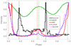 |
Fig. 1. Time lags between peaks in the different wavelengths. Radio pulse profiles are in red for NRT, in dashed blue for LOFAR, and in dotted magenta for NenuFAR, while thermal X-ray profiles are in green, and Fermi/LAT profiles are in black. The dashed coloured vertical lines show the phase of the peak flux of each pulse. |
The NICER X-ray data analysed as part of this work were recorded more recently, as further described in Sect. 2.2. We therefore used NRT data to build another timing solution for PSR J0030+0451, contemporaneous with the NICER data. The radio data considered in this new analysis were recorded with the Nançay Ultimate Pulsar Processing Instrument (NUPPI) backend (a version of the Green Bank Ultimate Pulsar Processing Instrument designed for the NRT), which replaced the BON backend as the principal pulsar timing instrument in operation at Nançay in August 2011. We used pulsar timing data recorded between August 2011 and April 2022. Although the two pulsar timing solutions described in this Section were obtained by analysing data from the same telescope, the two timing solutions were obtained from two separate analyses; therefore, the two ephemerides did not necessarily assume a common reference phase for the radio pulse profiles. We compared the BON and NUPPI reference profiles to determine the offset between the two reference phases. This phase offset of ∼0.056 was added to the NICER photon phases in order for the radio, X-ray, and γ-ray pulse profiles to share a common phase reference.
2.1.2. LOFAR
We also observed J0030+0451 using the international LOw Frequency ARray (LOFAR) station SE607 in Onsala, Sweden. LOFAR is fully described in Stappers et al. (2011) and van Haarlem et al. (2013). LOFAR stations have two different frequency bands: we used the HBA band, for which the station consists of 96 antenna tiles. Each of these tiles is made up of 16 dual-polarisation antenna elements. For each tile, an analogue sum is performed. The tile signals are then digitised and added numerically to form a coherent beam. For this project, we recorded data between 110.0 and 187.9 MHz. We refolded the LOFAR observations using the NUPPI timing solution, except for the dispersion measure, for which we directly calculated one DM value per LOFAR observation. We combined 168 observations recorded between 2019 and 2023, correcting for time-dependent DM variations.
2.1.3. NenuFAR
We also observed J0030+0451 using the new low-frequency radio telescope NenuFAR (New extension in Nançay upgrading LOFAR; see Zarka et al. 2015, 2020). NenuFAR is a compact phased array and interferometer formed of hexagonal groups of 19 dual-polarisation antennas called mini-arrays. It is located in Nançay, and operates in the 10–85 MHz frequency range. We used the dedicated pulsar instrumentation UnDysPuTeD and associated software LUPPI. This latter is based on NUPPI, and is designed to dedisperse and fold pulsar observations in real time, with up to four bands of 37.5 MHz simultaneously (Bondonneau et al. 2021). NenuFAR is an array of antennas that has been rolled out in several construction phases since the start of its observations in 2019. Observations in 2019–2022 used 56 mini-arrays, and observations in 2022–2023 used 80 mini-arrays, of which a minimum of 75 are active at any point; that is, ≥1425 antennas in total, allowing for sensitive observations (Pétri et al. 2023). We recorded data between 20.3 and 84.3 MHz; in the final analysis, we only kept data above 42 MHz as scattering started to considerably affect the profile shape at the lowest frequencies. We refolded the NenuFAR observations using the NUPPI timing solution, except for the DM value, for which the value determined directly from the NenuFAR observations is considerably more precise owing to the low-frequency coverage of NenuFAR. We combined 95 observations, correcting for time-dependent DM variations. We then added a constant phase offset to the NenuFAR observations to correct for different instrumental delays between NenuFAR and NUPPI.
J0030+0451 is among the twelve MSPs detected by NenuFAR, see Bondonneau et al. (2021, and in prep.). The NenuFAR profile of the pulsar differs from that obtained by NRT, but the two profiles are of comparable width. Furthermore, our observations are compatible with the radio emission detected by NenuFAR and NRT being emitted at the same rotational phase as the pulsar.
2.2. Thermal X-ray pulse profile with NICER data
The thermal X-ray pulse profile was obtained from NICER observations of PSR J0030+0451. We used all available data from 2017-07-24 20:36:00 to 2022-02-12 15:10:00, corresponding to ObsIDs 1060020101 to 4060020619. To process the data, we employed the standard recipes with nicerl2 (from NICERDAS v9 distributed with HEASOFT 6.30 and NICER calibration file v20210707). Furthermore, we used the NICERsoft2 suite to perform additional filtering, with the following criteria beyond the default ones. We excluded detector #34, which is known to be particularly noisy; we excluded portions of the NICER orbit during which the Earth magnetic cut-off rigidity was lower than 1.5 GeV c−1 at the satellite’s location. We also restricted the data to observing times when the space weather index KP was lower than 5, and when undershoot was lower than 200 c s−1 (see the NICER Data analysis threads3 for detailed description of these filtering criteria).
The NICERsoft package was also used to merge the event files into a single event file. Finally, we also performed a count rate cut on the merged event file, first when detector #14 (also known to be intermittently noisy) had a count rate above 1 c s−1 (with 8-s time bins), and second when the total count rate (all remaining detectors) was larger than 6 c s−1, in order to remove generally noisy time intervals remaining after the filtering described above. The phases of all events were calculated with the photonphase task of the PINT package4, and using the NUPPI ephemeris, including a phase offset of ∼0.056, as described in Sect. 2.1.
Given the relative faintness of thermal X-ray emission of MSPs compared to the background level of NICER observations, we also calculated the optimal energy range that maximises the detection of the pulsations (see Guillot et al. 2019 for the description of this optimisation). This energy range will vary from pulsar to pulsar, and depends on the spectral shape of the pulsar, the energy range where the NICER effective area is the largest, and on the overall background spectral shape of the observations (which can vary depending on the strength of the various background components). For PSR J0030+0451, we find an optimal energy range of 0.28–1.46 keV, giving a detection significance of 223 sigma. The pulse profile is shown in Fig. 1.
2.3. γ-ray pulse profile
Similar to the BON radio pulse profile for PSR J0030+0451 displayed in Fig. 1, the γ-ray pulse profile was taken from the 2PC auxiliary files archive. The profile, also displayed in Fig. 1, was constructed as part of the preparation of 2PC by analysing γ-ray photons recorded by the Fermi Large Area Telescope (LAT) between 2008 August 4 and 2011 August 4. We selected γ-ray photons with reconstructed energies from 0.1 to 100 GeV and phase-folded them with the BON ephemeris for PSR J0030+0451 as described in Sect. 2.1.
3. Determination of the pulsar magnetic field
Based on the radio and γ-ray data, Pétri (2011) previously investigated the geometry of the dipole magnetic field of PSR J0030+0451 with the striped wind model, relying on the split monopole configuration introduced by Bogovalov (1999). More recently, Benli et al. (2021) used the force-free magnetosphere solution for the special class of millisecond pulsars. In the latter work, the best-fit parameters were found to be around α = 70° and ζ = 60°, where α is the magnetic obliquity and ζ is the line-of-sight inclination angle relative to the spin axis. In the following section, we re-explore these results, showing several possible configurations for the joint radio and γ-ray light-curve fitting. We then constrain the off-centred position of the dipole from the location and shape of the thermal X-ray hot spot.
3.1. Dipole geometry from joint radio and γ-ray modelling
The light-curve fitting procedure was explained in depth by Benli et al. (2021) and Pétri & Mitra (2021). We simply recall that the two main characteristics to be adjusted are the γ-ray peak separation Δ and the phase lag between the first γ-ray peak and the peak of the radio profile δ. To very good approximation, with an error of less than 1%, Pétri (2011) showed that this relation is

For PSR J0030+0451, the second Fermi pulsar catalogue (Abdo et al. 2013) reports a value for the phase separation between the two γ-ray peaks of Δ = 0.450, and a γ-ray lag of the first γ-ray peak with respect to the peak of the radio profile of δ = 0.146. Additionally, the NICER Collaboration reports a value of ζ = 54° (Riley et al. 2019). This would imply an obliquity of α = 78°, which is not far from the independent γ-ray light-curve fitting performed by Benli et al. (2021), who found α = 70°. Using the input from the thermal X-ray detailed in Sect. 3.2, we were also looking for solutions of the γ-ray light curves by constraining the line-of-sight inclination to ζ = 54° or to ζ = 50° as given by the NICER Collaboration.
To find a good fit to the data, we minimise a kind of reduced  value, which is defined as
where N is the number of data points, ν = N − 2 the degree of freedom,  the observed γ-ray flux,
  the predicted γ-ray flux, and σi the uncertainties in the gamma-ray flux. There are two parameters to adjust, the magnetic obliquity and the inclination of the line of sight. The most important characteristics of our model are the γ-ray peak separation Δ and the γ-ray lag δ. Our model does not produce off-pulse emission. Therefore, we select only the phase intervals containing the two peaks, as shown in the grey boxes in Fig. 2. All light curves are plotted in arbitrary units, applying a normalisation such that the peak value in each energy band is unity. The best values for the parameters α and ζ and the shift in phase ϕs are those minimising the
  . Two possible fits are shown in Fig. 2 and agree reasonably well between radio, γ-rays, and the geometry constrained from thermal X-rays. We found α = 75° and ζ = 54° for the upper panel and α = 70° and ζ = 60° for the lower panel. These results rely on a centred dipole, and therefore entail the assumption that the radio and γ-ray emission emanate from high altitude, where the perturbation of surface fields and the off-centering of the large-scale dipole become imperceptible due to the faster decrease in these components with distance. We next show how to determine the close region field structure, where the off-centred position of the large-scale dipole is crucial for the thermal surface emission.
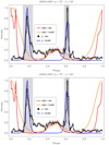 |
Fig. 2. Some fits for the radio and γ-ray light curves of PSR J0030+0451. The parameters used are α = 75° and ζ = 54° in the top panel and α = 70° and ζ = 60° in the bottom panel. The grey boxes show the phase intervals used for the γ-ray fit. |
3.2. Off-centred dipole geometry from thermal X-rays
We constrain the geometry of the off-centred large-scale dipole from both the location and size of the two polar caps – which are deduced from the NICER observations of Riley et al. (2019) and Miller et al. (2019) – and the half-opening angles of the cones subtending their rims. Figure 3 highlights the geometry and shows the relevant angles and axes. Let us assume that the centre of the northern polar cap is located at the point N with spherical coordinates (R, θn, ϕn) and the position vector given by Rn = R n and similarly for the southern polar cap at point S with coordinates (R, θs, ϕs) and a position vector Rs = R s, where R is the neutron star radius. Here, n and s are therefore unit vectors pointing towards the centre of the hot spots. Let us also denote the unit vector joining both polar cap centres by

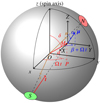 |
Fig. 3. Geometry of the off-centred dipole, showing the location of the hot spots N and S and the angles defined in the text (α, δ, β). |
The obliquity of the magnetic dipole is therefore given by projection onto the rotation axis ez according to
We choose the solution corresponding to α ∈ [0, π/2]. The minimal distance of the line joining N and S to the centre of the neutron star is given by
This point on the segment NS is denoted M. Equation (5) gives a lower bound to the distance d from the magnetic dipole moment location to the star centre. Were the dipole located at any other point along the segment joining point N to point S, the distance d between the dipole position M and the centre of the star O would be larger. The angle between the line joining the dipole moment to the star centre and the rotation axis is

where  and
and  . The angle β is the angle between the vector
  projected onto the plane (xOy) – written as
  – and the vector joining S and N, thus n − s or the unit vector t,
The relative angular size difference between the northern and the southern hot spot region helps us to constrain the location of the magnetic dipole along the line joining the two poles N and S. Indeed, knowing the northern and southern polar cap radius, denoted ξn and ξs respectively, their ratio ξn/ξs is related to the distance d between the location of the dipole moment and the centre of the star. For instance, for an aligned rotator, if the dipole is located at the stellar centre, this ratio is equal to unity because both spots are identical. Moreover, using a spherical coordinate system (r, θ, ϕ), the field lines are given by r = λ rLsin2θ with rL = c/Ω the light-cylinder radius, c the speed of light, Ω the stellar spin frequency, and λ a parameter labelling each field line. However, already when the dipole is shifted along the rotation axis, the geometry becomes asymmetrical, and one spot grows while the second shrinks. More quantitatively, the half-opening angle ξ (northern or southern spot) is the solution to the transcendental equation
with a = R/rL and

where θ0 and ϕ0 are the spherical polar colatitude and azimuth of the magnetic moment position, respectively. For an arbitrary location of this magnetic moment, even for an aligned rotator, the polar cap shapes deviate from a circular rim and the axial symmetry is broken. Therefore, we need to solve for the radius at each azimuth ϕ in order to deduce the opening angle ξ for any given ϵ and a. We need to find the roots ξ(ϕ) of Eq. (8). The sign of λ is arbitrary because the solution always shows a symmetry between the north pole and the south pole. For a centred dipole ϵ = 0 and λ = 1,  , as is well known. A similar computation could be done with an orthogonal static rotator. The polar cap shape is then given by Pétri (2018) and depends on the angle ϕ. We do not enter into such complications because accurate determination of the rims would require a full force-free numerical simulation of the magnetosphere, which is too computationally expensive in regard to the number of free parameters to explore. However, the aligned case already provides good insight into the impact of off-centring on the respective sizes of the polar caps.
In the particular case of the millisecond pulsar PSR J0030+0451, the ratio of stellar radius to light-cylinder radius is a = R/rL ≈ 0.055 according to Riley et al. (2019), who found an estimate of its radius  km and its mass
  . The offset value ϵ = d/R required to adjust the relative spot angular sizes for different values of α and ϕ according to Eq. (8) is shown in Fig. 4. Here, θ0 and ϕ0 in the legend are given in units of π/4 for several different values spanning the range [0, π] in steps of k π/4 with k ∈ [0..4]. Because some curves overlap, they are not all shown. A ratio ξs/ξn of larger that 4 requires an offset of as high as ϵ ≳ 0.9. A ratio ξs/ξn equal to unity means that the two spots are of equal size. Figure 4 shows the ratio ξs/ξn in log scale. We notice that this plot is symmetric with respect to the x-axis. Translated into the ratio ξs/ξn, this means that for each value of displacement ϵ there exists a value r1 of the ratio ξs/ξn = r1 with a position of the magnetic moment at (θ1, ϕ1) associated to the inverse ratio ξs/ξn = 1/r1 with a new position of the magnetic moment given by the angles (θ2, ϕ2), which are uniquely related to (θ1, ϕ1). Such symmetry is expected because of the symmetric nature of the magnetic dipole with respect to the inversion between north pole and south pole. These values could differ for a more realistic force-free field, but we also expect large offsets for large differences in spot sizes.
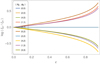 |
Fig. 4. Ratio ξs/ξn of the polar cap half-opening angles of the south and north pole (respectively ξs and ξn) as a function of the fractional offset from the centre ϵ = d/R. The colours correspond to different values of the angles (θ0, ϕ0) in units of π/4. |
The fit parameters of Riley et al. (2019) are summarised in Table 1, which shows some of the models used by these authors. Among others, these are the single temperature+protruding single temperature (ST+PST), the single temperature+eccentric single temperature (ST+EST), the single temperature+concentric single temperature (ST+CST), the single temperature unshared parameters (ST-U), and the concentric dual-temperature unshared parameters (CDT-U). The geometry of the off-centred dipole with (α, β, δ, ϵ) is then deduced and shown in the right columns in the same table.
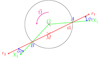 |
Fig. 5. Geometry explaining the time lag between the radio peaks and the X-ray peaks and depicted by the angles ϕ1 and ϕ2. |
Off-centred dipole geometry deduced from the polar cap location after Riley et al. (2019).
Independent constraints from a second group (Miller et al. 2019) are reported in Table 2 for a two-spot and a three-spot model5. The line “3 spot1” considers only the first and second spot and the line “3 spot2” considers the first and third spots to find the geometry of the off-centred dipole. The line “3 mean” interprets the last two hot spots as emanating from the same polar cap where the centre is approximately located halfway between the two spot centres (Θp + Θs)/2 and (ϕp + ϕs)/2 (which is an approximation of the exact middle joining both centres on the sphere). With this assumption, we obtain other parameters that better agree with the two-spot model referred to as ST+PST in Table 1.
Off-centred dipole geometry deduced from the polar cap location after Miller et al. (2019).
3.3. X-ray and γ-ray time lag
Our light-curve fitting procedure relies heavily on the phase-aligned pulse profiles. The most important characteristics of these pulse profiles are the phases of the peaks in γ-ray and X-ray. For the radio pulse profile, we prefer to use the centre of the radio pulse as the reference phase. We think indeed that the centre is more robust, because it relies on a geometrical estimate not related to the flux of the radio emission that can strongly vary between components. We define the centre of the pulse to be at a phase halfway between the phases of 10% of the maximum flux of the corresponding pulse. The three light curves for radio, thermal X-ray, and γ-ray are shown in Fig. 1 with vertical dashed lines depicting the phase of the midpoint at 10% maximum values for each pulse; see the values in Table 3.
Phase location of the first and second peak in radio, X-ray, and γ-ray.
The first X-ray pulse peak arrives slightly before the pulse in the radio pulse profile, whereas the second X-ray peak slightly lags the second radio pulse by a phase difference of about Δϕ ≈ ±0.025. This ordering is compatible with the off-centred dipole geometry because the order of appearance of radio and X-rays is inverted between the north and south pole for polar caps with a simple circular shape. According to Riley et al. (2019) and Miller et al. (2019), even for PSR J0030+0451, for which one pole differs significantly from a circular shape, the inversion in the phase lag between the two wavelengths holds.
The phase lag between the radio peak and the X-ray peak is produced as follows: on one hand, for a circular hot spot on the stellar surface, assuming constant and isotropic emissivity, the maximum X-ray flux is observed when the line of sight, the normal to the centre of the hot spot, and the rotation axis are all coplanar. On the other hand, the radio flux peaks whenever the tangent to the magnetic field line at the emission point lies in the plane defined by the rotation axis and the line of sight. Because the field lines are usually curved and not pointing in the radial direction, we expect a shift in phase between X-rays and radio. The most important factors here are the projection of the magnetic moment and the position vectors of the hot spot centres onto the equatorial plane, that is, the points A and B as shown in Fig. 5. The straight red line corresponds to the projection of the magnetic moment. The two green lines depict the projection of the vector position s and n. The star is rotating anticlockwise. The first radio peak r1 leads the first X-ray peak X1 by a phase shift ϕ1. However, the second radio peak r2 trails the second X-ray peak X2, separated by a phase shift ϕ2. The first and leading radio peak has switched to a second and trailing radio peak. This configuration holds in almost all cases, with the exception being when the projected magnetic axis passes by the origin O. In such a case, the time lag vanishes and the pulse peaks are aligned.
A last important point concerns the phase lag between radio and X-rays, which is not taken into account by the thermal X-ray fitting only. The peaks in X-ray are almost aligned with the centre of the radio pulse (Table 3) with a time lag of only 0.02 − 0.03 in phase.
Figure 6 shows the different locations of the hot spots projected onto the equatorial plane as deduced from Table 1. They all give very similar directions of radio and X-ray emission phase of ϕ1 ≈ 6° and ϕ2 ≈ −10°. Only the ST+PST model produces larger time lags of ϕ1 ≈ 8° and ϕ2 ≈ −26°. The precise values are summarised in Table 4. We highlight the change in sign between ϕ1 and ϕ2 because of the switch from lagging to leading peak. The phase lags in units of the rotation period are of the order ϕ2 ≈ −0.03 and ϕ1 ≈ 0.02, and are in good agreement with the time lag in Fig. 1.
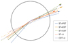 |
Fig. 6. Time lag as expected from the NICER observations. The dashed coloured lines correspond to the direction of the magnetic axis, whereas the solid coloured lines show the direction of the normal for each hot spot, all directions being projected onto the equatorial plane. |
Accurately estimating the expected phase lag requires a more quantitative geometric study of the location of the peak X-ray emission within the hot spot, as well as a careful analysis of aberration, retardation, and magnetic sweep-back effects in the different wavelengths (Phillips 1992). Close to the neutron star, especially for the thermal X-ray emission, light-bending and the Shapiro delay should be included too. However, this is beyond the scope of this work.
Our multi-wavelength analysis and NICER thermal X-ray pulse profile fitting independently lead to a line-of-sight inclination angle of ζ = 54°. As a consequence, we take this value as a robust estimate of ζ. Therefore, from relation (1), we find α ≈ 78°, in accordance with our γ-ray fit of 75°. We then take α ≈ 75° as another robust result.
3.4. Small-scale surface dipole
The two independent groups working on the thermal X-ray pulse profile modelling fitted the hot spot emission with different patches: circular shapes for Riley et al. (2019) or ovals for Miller et al. (2019), with these latter authors finding three possible hot spots. The rim of these polar caps must somehow be related to the surrounding magnetosphere, which is connected to the relativistic plasma flow hitting and heating the surface. It is well known that radio emission physics requires strong curvature field lines to produce sufficient electron–positron pairs and the associated radiation. This can only be achieved by small-scale surface magnetic fields locally dominating the global dipole field, possibly off-centred as discussed for instance by Szary (2013). In this section, we show that a small-amplitude surface magnetic dipole located slightly inside the neutron star crust (at a distance of 0.05 R below the surface) on top of a large-scale off-centred dipole field can lead to polar cap shapes similar to those expected from the NICER observations.
There are several free parameters with which to specify each dipole configuration, making it impossible to explore the full parameter space with high resolution and realistic magnetospheres filled with a pair plasma. Instead, here we only provide a ‘proof of concept’ for this idea, using a static vacuum dipole geometry and neglecting the displacement current. As the components of the total magnetic field (off-centred dipole and small-scale surface dipole) are known, we compute the field line structure by straightforward integration for a sample of representative lines. Each field line crossing the light cylinder is reputed to be part of the open region where the plasma flows (Pétri 2016). Their foot points are connected to the hot spots. Figure 7 shows an example of a two-spot configuration, both poles being located in the southern hemisphere, one with a small, almost circular shape and the other much more elongated and thin, with a crescent shape, as reported in Riley et al. (2019). To obtain these shapes, the parameters used in the figure are as follows: a large-scale magnetic moment inclination angle of α0 = 75° and a position vector (x0, y0, z0) = (0, 0, −0.8) R; a ratio between the small-scale dipole B1 and the large-scale dipole B0 given by B1/B0 = 0.3; a position vector of the small dipole (x1, y1, z1) = (−0.4, −0.6, −0.6) R; and an inclination angle of the small dipole amounting to α1 = 150°. However, we note that the quantitative pictures do not agree as we are not attempting to accurately model the hot spots because of our very restrictive assumptions of an empty and static magnetosphere.
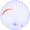 |
Fig. 7. Three-dimensional view of the two hot spots from the south pole. These are produced by a large-scale off-centred dipole and a small-scale surface dipole located close to one magnetic pole. |
4. Discussion
On one hand, joint radio and γ-ray fitting constrains the two important angles, namely the line-of-sight inclination and magnetic dipole moment inclination. On the other hand, thermal X-ray pulse profiles from the surface determine the location of the hot spots and their shape. Combining both approaches in a unified framework would better constrain the priors used in the procedure of thermal X-ray fitting. Indeed, from a theoretical point of view, the heating of the stellar surface seen as hot spots must be connected to the surrounding magnetospheric activity related to pair cascades and particle bombardments. From an observational point of view, the knowledge gained from the γ-ray fitting would pin down the line-of-sight inclination angle and the large-scale dipole obliquity, narrowing the allowed parameter space within which we search with the thermal X-ray pulse profile fitting.
However, a severe limitation to this approach is the number of free parameters to be added to describe the magnetic field topology. We can model the field with for instance two dipoles or a dipole plus some quadrupolar components but the number of free parameters to adjust would be similar. The thermal X-ray hot spot geometry supports the idea of an off-centred dipole locally disturbed by a small-scale dipole on the surface. However, we are far from a precise quantitative picture because this would require the simulation of a large sample of force-free magnetospheres with dipole+dipole fields to span a reasonable range of the space parameter. In the current stage, this is computationally unfeasible, except if the region to search for is already small enough with only a dozen runs to perform.
Oblateness is also neglected in our study; we assumed a perfect spherical body. According to Silva et al. (2021), the perturbation induced by the rotation of a 200 Hz neutron star like PSR J0030+0451 is weak, and the ratio between the equatorial and polar radii is expected to be between 1 and 1.04, which is within the acceptable size limit for the qualitative study performed in this work; see for instance the vacuum and force-free oblate and prolate solutions found by Pétri (2022a,b).
Due to the presence of an interpulse component in its pulse profile, PSR J0030+0451 is assumed to be an approximately orthogonal rotator with a line of sight close to the equatorial plane, that is, ζ ∼ 90°. However, the parameters found by the NICER Collaboration and by our radio/γ-ray fit show that the line of sight is closer to ζ = 54°. This means that the radio beam cone opening angle must be large. Assuming a dipolar magnetic field structure at the radio emission site, we can estimate the emission height. Indeed, the opening angle θem of the emission cone along the magnetic field lines at the surface is (Gangadhara & Gupta 2001):
The north pole is visible only if ζ ∈ [α − θem, α + θem] ≈ [55° ,95° ] which is very close to the lower limit for ζ. For the south pole to become visible, we moreover require that ζ ∈ [π − α − θem, π − α + θem] ≈ [85° ,125° ], which is clearly not the case. In order to reconcile the geometry with observations, the photon emission site for radio has to be shifted to higher altitudes of around rem ≈ 6 R. In this case, the new cone opening angle becomes  . Now the line of sight inclination angle must lie within
 ![$ \zeta \in [\alpha - \theta_{\rm em}^*, \alpha + \theta_{\rm em}^*] \approx [22^{\circ}, 127^{\circ}] $](/articles/aa/full_html/2023/12/aa46913-23/aa46913-23-eq23.gif) and
and ![$ \zeta \in [\pi - \alpha - \theta_{\rm em}^*, \pi - \alpha + \theta_{\rm em}^*] \approx [52^{\circ}, 157^{\circ}] $](/articles/aa/full_html/2023/12/aa46913-23/aa46913-23-eq24.gif) , just on the boundary of the interval to observe the south pole. This altitude would correspond to a significant fraction of the light-cylinder radius of about 6 R/rL ≈ 1/3. Nevertheless, the presence of a small-scale surface dipole could alter the direction of radio emission of the crescent-shaped pole if photons are produced relatively close to the surface, possibly shifting the emission height to lower altitudes and then seen at different phases. This could also change the radio peak separation in our model, where we used a simple centred dipole in Fig. 2. Looking at the width of both radio pulses, they are about 110 − 120°, which means a half-opening angle of the emission cone of about θem ∼ 55 − 60°. This agrees with the above estimate to see both pulses when ζ ≈ 54°. Consequently, there is a convergence towards the fact that the radio emission emanates from high altitude, close to the light cylinder in an almost dipolar region.
, just on the boundary of the interval to observe the south pole. This altitude would correspond to a significant fraction of the light-cylinder radius of about 6 R/rL ≈ 1/3. Nevertheless, the presence of a small-scale surface dipole could alter the direction of radio emission of the crescent-shaped pole if photons are produced relatively close to the surface, possibly shifting the emission height to lower altitudes and then seen at different phases. This could also change the radio peak separation in our model, where we used a simple centred dipole in Fig. 2. Looking at the width of both radio pulses, they are about 110 − 120°, which means a half-opening angle of the emission cone of about θem ∼ 55 − 60°. This agrees with the above estimate to see both pulses when ζ ≈ 54°. Consequently, there is a convergence towards the fact that the radio emission emanates from high altitude, close to the light cylinder in an almost dipolar region.
Inspecting the NenuFAR radio pulse profile in Fig. 1, we observe that the emission in both radio peaks is almost phased-aligned with their NRT counterpart (see Table 3). Moreover, the second radio peak pulse width is comparable to the NRT width and located at the same phases. However, the first peak seems to depart slightly from its NRT counterpart; its width is larger and it leads the high frequency counterpart by 3% in phase. This suggests that both radio bands are produced at approximately the same altitude within the magnetosphere. The same conclusion holds for the LOFAR observations; the widths of the pulses are similar to those seen by NenuFAR, although their shapes differ, especially for the weaker pulse around phase 0.5. More specifically, because of the small size of the light cylinder, which is only rL ≈ 18.3 R, there is indeed not a significant amount of space left to span a vast range in emission height. Moreover, the morphology of the first peak changes at low frequency, highlighting a possible change in the local magnetic field geometry at the altitude where these photons are produced due to the small-scale surface dipole. Indeed, Riley et al. (2019) points out that the first X-ray pulse profile belongs to the crescent-shaped hot spot. In the picture formed from our findings, this is related to a small-scale surface dipole that then also impacts the radio emission properties between the NenuFAR and NRT frequencies.
5. Conclusions
With the increase in sensitivity of telescopes at all wavelengths, the simultaneous fitting of radio, X-ray, and γ-ray light curves of pulsars becomes a very powerful tool with which to constrain the locations of the emission regions, the magnetic dipole obliquity, and the observer line-of-sight inclination angles. For PSR J0030+0451, we show that thermal X-ray pulse profile fitting in conjunction with a joint radio and γ-ray light-curve fitting gives very similar expectations for those angles. This supports the idea that radio and γ-ray emission models for young pulsars apply equally well to recycled millisecond pulsars, even if the presence of multipolar fields could strongly impact the surface emission and to a lesser extent the radio and γ-ray radiation. We find that α ≈ 75° and ζ ≈ 54° are very robust results for the multi-wavelength light curves of PSR J0030+0451.
The above study verifies the consistency between both approaches without exploring a precise description of the magnetic configuration. To go further would require a more quantitative analysis, performing numerical simulations of off-centred force-free dipolar magnetospheres on top of small-scale surface dipoles. Unfortunately, the total number of parameters makes this computationally intractable because of the huge number of configurations to explore. It is therefore compulsory to narrow down the region of interest in the parameter space for each individual pulsar, as done in the present work.
The concomitance between the two independent results in X-ray and radio/γ-ray may simply be a coincidence. But with the ongoing NICER campaign, the number of pulsars with confident hot spot modelling will increase and such a chance occurrence could be rejected with ever increasing confidence. Therefore, our next target is PSR J0740+6620 (Miller et al. 2021; Riley et al. 2021), which shows very similar behaviour to PSR J0030+0451. Results will be discussed in an upcoming paper.
Last, but not least, millisecond pulsars might emit thermal X-rays that are polarised. The recent discussion by Suleimanov et al. (2023) based on a self-consistent atmosphere model in local thermodynamic equilibrium shows that for an unmagnetised neutron star with a hydrogen or carbon atmosphere, the maximum polarisation degree can reach 25% and 40%, respectively. Moreover, it is possible for the X-ray emission to become substantially polarised if multipolar components are present, with magnetic field strength exceeding B ∼ 106 T (see for example spectra and polarisation of magnetised neutron stars in Lloyd 2003). Including polarisation degree and polarisation angle in the analysis could provide two additional dimensions, helping to break the degeneracy in the parameter space and disentangle the surface magnetic field structure. This kind of study would be particularly relevant in the context of future X-ray polarimetry missions with sensitivity of around 0.1–1 keV6.
However, as noted in Miller et al. (2019), the three-spot model is not statistically preferable to the two-spot model; the log-likelihood of the former being only 1.7 higher than that of the latter, which is a difference of smaller than the uncertainties on the log-likelihood. In other words, both models are equally good descriptions of the data.
We note that millisecond pulsars are too faint to be detectable by current X-ray polarimetry observatories, such as the Imaging X-ray Polarimetry Explorer mission (IXPE, Weisskopf et al. 2022), which operates in the 2 − 8 keV range.
Acknowledgments
We are grateful to the referee for helpful comments and suggestions and to David Smith for useful discussions. This work has been supported by the CEFIPRA grant IFC/F5904-B/2018 and ANR-20-CE31-0010 (MORPHER). S.G., N.W. and D.G.C. acknowledge the support of the CNES. We acknowledge the use of the Nançay Data Center computing facility (CDN – Centre de Données de Nançay). The CDN is hosted by the Nançay Radio Observatory in partnership with Observatoire de Paris, Université d’Orléans, OSUC and the CNRS. The CDN is supported by the Region Centre Val de Loire, département du Cher. The Nançay Radio Observatory is operated by the Paris Observatory, associated with the French Centre National de la Recherche Scientifique (CNRS). We acknowledge financial support from the “Programme National de Cosmologie et Galaxies” (PNCG) and “Programme National Hautes Energies” (PNHE) of CNRS/INSU, France. This paper is partially based on data obtained using the NenuFAR radio-telescope. The development of NenuFAR has been supported by personnel and funding from: Nançay Radio Observatory (ORN), CNRS-INSU, Observatoire de Paris-PSL, Université d’Orléans, Observatoire des Sciences de l’Univers en région Centre, Région Centre-Val de Loire, DIM-ACAV and DIM-ACAV+ of Région Ile de France, Agence Nationale de la Recherche. LOFAR, the Low-Frequency Array designed and constructed by ASTRON, has facilities in several countries, that are owned by various parties (each with their own funding sources), and that are collectively operated by the International LOFAR Telescope (ILT) foundation under a joint scientific policy. The observations used in this work were made during ILT time allocated under the long-term pulsar monitoring campaign (projects LC0_014, LC1_048, LC2_011, LC3_029, LC4_025, LT5_001, LC9_039, LT10_014, LC14_012, LC15_009, LT16_007 and LC20_014). We acknowledge support from Onsala Space Observatory for the provisioning of its facilities/observational support. The Onsala Space Observatory national research infrastructure is funded through Swedish Research Council grant No 2019-00208. I.P.K. acknowledges the support of Collége de France by means of “PAUSE–Solidarité Ukraine” and of NAS of Ukraine by a Grant of the NAS of Ukraine for Research Laboratories/Groups of Young Scientists of the NAS of Ukraine (2022–2023, project code “Spalakh”).
References
- Abdo, A. A., Ajello, M., Allafort, A., et al. 2013, ApJS, 208, 17 [Google Scholar]
- Bauböck, M., Psaltis, D., & Özel, F. 2019, ApJ, 872, 162 [CrossRef] [Google Scholar]
- Benli, O., Pétri, J., & Mitra, D. 2021, A&A, 647, A101 [NASA ADS] [CrossRef] [EDP Sciences] [Google Scholar]
- Bilous, A. V., Watts, A. L., Harding, A. K., et al. 2019, ApJ, 887, L23 [NASA ADS] [CrossRef] [Google Scholar]
- Bogovalov, S. V. 1999, A&A, 349, 1017 [Google Scholar]
- Bogdanov, S., Grindlay, J. E., & Rybicki, G. B. 2008, ApJ, 689, 407 [Google Scholar]
- Bondonneau, L., Grießmeier, J.-M., Theureau, G., et al. 2021, A&A, 652, A34 [NASA ADS] [CrossRef] [EDP Sciences] [Google Scholar]
- Carrasco, F., Pelle, J., Reula, O., Viganò, D., & Palenzuela, C. 2023, MNRAS, 520, 3151 [NASA ADS] [CrossRef] [Google Scholar]
- Chen, A. Y., Yuan, Y., & Vasilopoulos, G. 2020, ApJ, 893, L38 [Google Scholar]
- Gangadhara, R. T., & Gupta, Y. 2001, ApJ, 555, 31 [NASA ADS] [CrossRef] [Google Scholar]
- Gil, J. A., Melikidze, G. I., & Mitra, D. 2002, A&A, 388, 235 [NASA ADS] [CrossRef] [EDP Sciences] [Google Scholar]
- Guillot, S., Kerr, M., Ray, P. S., et al. 2019, ApJ, 887, L27 [Google Scholar]
- Johnson, T. J., Venter, C., Harding, A. K., et al. 2014, ApJS, 213, 6 [Google Scholar]
- Kalapotharakos, C., Wadiasingh, Z., Harding, A. K., & Kazanas, D. 2021, ApJ, 907, 63 [NASA ADS] [CrossRef] [Google Scholar]
- Lloyd, D. A. 2003, Ph.D. Thesis, Harvard University, USA [Google Scholar]
- Miller, M. C., Lamb, F. K., Dittmann, A. J., et al. 2019, ApJ, 887, L24 [Google Scholar]
- Miller, M. C., Lamb, F. K., Dittmann, A. J., et al. 2021, ApJ, 918, L28 [NASA ADS] [CrossRef] [Google Scholar]
- Mitra, D. 2017, J. Astrophys. Astron., 38, 52 [NASA ADS] [CrossRef] [Google Scholar]
- Phillips, J. A. 1992, ApJ, 385, 282 [NASA ADS] [CrossRef] [Google Scholar]
- Pétri, J. 2011, MNRAS, 412, 1870 [Google Scholar]
- Pétri, J. 2016, J. Plasma Phys., 82, 635820502 [CrossRef] [Google Scholar]
- Pétri, J. 2018, MNRAS, 477, 1035 [Google Scholar]
- Pétri, J. 2019, MNRAS, 485, 4573 [CrossRef] [Google Scholar]
- Pétri, J. 2022a, A&A, 659, A147 [NASA ADS] [CrossRef] [EDP Sciences] [Google Scholar]
- Pétri, J. 2022b, A&A, 657, A73 [NASA ADS] [CrossRef] [EDP Sciences] [Google Scholar]
- Pétri, J., & Mitra, D. 2021, A&A, 654, A106 [NASA ADS] [CrossRef] [EDP Sciences] [Google Scholar]
- Pétri, J., Guillot, S., Guillemot, L., et al. 2023, Constraining the magnetic field of the millisecond pulsar PSR J0030+0451 from joint radio, thermal X-ray and γ-ray emission. Supplementary Material: List of NenuFAR Observations (version 1.0) (PADC), https://doi.org/10.25935/04q0-t518 [Google Scholar]
- Radhakrishnan, V., & Cooke, D. J. 1969, Astrophys. Lett., 3, 225 [NASA ADS] [Google Scholar]
- Riley, T. E., Watts, A. L., Bogdanov, S., et al. 2019, ApJ, 887, L21 [Google Scholar]
- Riley, T. E., Watts, A. L., Ray, P. S., et al. 2021, ApJ, 918, L27 [CrossRef] [Google Scholar]
- Ruderman, M. 1991, ApJ, 366, 261 [CrossRef] [Google Scholar]
- Salmi, T., Suleimanov, V. F., Nättilä, J., & Poutanen, J. 2020, A&A, 641, A15 [NASA ADS] [CrossRef] [EDP Sciences] [Google Scholar]
- Silva, H. O., Pappas, G., Yunes, N., & Yagi, K. 2021, Phys. Rev. D, 103, 063038 [NASA ADS] [CrossRef] [Google Scholar]
- Stappers, B. W., Hessels, J. W. T., Alexov, A., et al. 2011, A&A, 530, A80 [NASA ADS] [CrossRef] [EDP Sciences] [Google Scholar]
- Suleimanov, V. F., Poutanen, J., Doroshenko, V., & Werner, K. 2023, A&A, 673, A15 [NASA ADS] [CrossRef] [EDP Sciences] [Google Scholar]
- Szary, A. 2013, ArXiv e-prints [arXiv:1304.4203] [Google Scholar]
- Sznajder, M., & Geppert, U. 2020, MNRAS, 493, 3770 [NASA ADS] [CrossRef] [Google Scholar]
- van Haarlem, M. P., Wise, M. W., Gunst, A. W., et al. 2013, A&A, 556, A2 [NASA ADS] [CrossRef] [EDP Sciences] [Google Scholar]
- Weisskopf, M. C., Soffitta, P., Baldini, L., et al. 2022, J. Astron. Telesc. Instrum. Syst., 8, 026002 [NASA ADS] [CrossRef] [Google Scholar]
- Yan, W. M., Manchester, R. N., van Straten, W., et al. 2011, MNRAS, 414, 2087 [NASA ADS] [CrossRef] [Google Scholar]
- Zarka, P., Tagger, M., Denis, L., et al. 2015, 2015 International Conference on Antenna Theory and Techniques (ICATT), 1 [Google Scholar]
- Zarka, P., Denis, L., Tagger, M., et al. 2020, URSI GASS 2020, Session J01 New Telescopes on the Frontier, https://tinyurl.com/ycocd5ly [Google Scholar]
All Tables
Off-centred dipole geometry deduced from the polar cap location after Riley et al. (2019).
Off-centred dipole geometry deduced from the polar cap location after Miller et al. (2019).
All Figures
|
Fig. 1. Time lags between peaks in the different wavelengths. Radio pulse profiles are in red for NRT, in dashed blue for LOFAR, and in dotted magenta for NenuFAR, while thermal X-ray profiles are in green, and Fermi/LAT profiles are in black. The dashed coloured vertical lines show the phase of the peak flux of each pulse. |
| In the text | |
|
Fig. 2. Some fits for the radio and γ-ray light curves of PSR J0030+0451. The parameters used are α = 75° and ζ = 54° in the top panel and α = 70° and ζ = 60° in the bottom panel. The grey boxes show the phase intervals used for the γ-ray fit. |
| In the text | |
|
Fig. 3. Geometry of the off-centred dipole, showing the location of the hot spots N and S and the angles defined in the text (α, δ, β). |
| In the text | |
|
Fig. 4. Ratio ξs/ξn of the polar cap half-opening angles of the south and north pole (respectively ξs and ξn) as a function of the fractional offset from the centre ϵ = d/R. The colours correspond to different values of the angles (θ0, ϕ0) in units of π/4. |
| In the text | |
|
Fig. 5. Geometry explaining the time lag between the radio peaks and the X-ray peaks and depicted by the angles ϕ1 and ϕ2. |
| In the text | |
|
Fig. 6. Time lag as expected from the NICER observations. The dashed coloured lines correspond to the direction of the magnetic axis, whereas the solid coloured lines show the direction of the normal for each hot spot, all directions being projected onto the equatorial plane. |
| In the text | |
|
Fig. 7. Three-dimensional view of the two hot spots from the south pole. These are produced by a large-scale off-centred dipole and a small-scale surface dipole located close to one magnetic pole. |
| In the text | |
Current usage metrics show cumulative count of Article Views (full-text article views including HTML views, PDF and ePub downloads, according to the available data) and Abstracts Views on Vision4Press platform.
Data correspond to usage on the plateform after 2015. The current usage metrics is available 48-96 hours after online publication and is updated daily on week days.
Initial download of the metrics may take a while.