| Issue |
A&A
Volume 673, May 2023
|
|
|---|---|---|
| Article Number | A53 | |
| Number of page(s) | 14 | |
| Section | Extragalactic astronomy | |
| DOI | https://doi.org/10.1051/0004-6361/202244080 | |
| Published online | 04 May 2023 | |
Probing quadratic gravity with the Event Horizon Telescope
1
Department of High Energy Physics/IMAPP, Radboud University, PO Box 9010 6500 GL Nijmegen, The Netherlands
2
Department of Astrophysics/IMAPP, Radboud University, PO Box 9010 6500 GL Nijmegen, The Netherlands
e-mail: This email address is being protected from spambots. You need JavaScript enabled to view it.
3
Department of Mathematics/IMAPP, Radboud University, PO Box 9010 6500 GL Nijmegen, The Netherlands
Received:
21
May
2022
Accepted:
24
November
2022
Abstract
Quadratic gravity constitutes a prototypical example of a perturbatively renormalizable quantum theory of the gravitational interactions. In this work, we construct the associated phase space of static, spherically symmetric, and asymptotically flat spacetimes. We find that the Schwarzschild geometry is embedded in a rich solution space comprising horizonless, naked singularities and wormhole solutions. Characteristically, the deformed solutions follow the Schwarzschild solution up outside of the photon sphere, while they differ substantially close to the center of gravity. We then carry out an analytic analysis of observable signatures accessible to the Event Horizon Telescope, comprising the size of the black hole shadow as well as the radiation emitted by infalling matter. On this basis, we argue that it is the brightness within the shadow region that constrains the phase space of solutions. Our work constitutes the first step towards bounding the phase space of black-hole-type solutions with a clear quantum gravity interpretation based on observational data.
Key words: black hole physics / gravitation / Galaxy: center / techniques: high angular resolution
© The Authors 2023
 Open Access article, published by EDP Sciences, under the terms of the Creative Commons Attribution License (https://creativecommons.org/licenses/by/4.0), which permits unrestricted use, distribution, and reproduction in any medium, provided the original work is properly cited.
This article is published in open access under the Subscribe to Open model. This email address is being protected from spambots. You need JavaScript enabled to view it. to support open access publication.
1. Introduction
General relativity constitutes the benchmark for describing gravitational phenomena. Its predictions have been confirmed in a vast number of experiments ranging from fundamental tests of the equivalence principle over the bending of light, the perihelion advance of mercury, and the Shapiro time delay, up to stellar system tests conducted within binary pulsar systems (Will 2014). In the last decade, the direct detection of gravitational waves emitted during the coalescence of binary black hole systems (Abbott et al. 2016), radio pulsar observations (Wex & Kramer 2020; Kramer et al. 2021), and the image of a black hole shadow (Falcke et al. 2000) taken by the Event Horizon Telescope (EHT) Collaboration (The Event Horizon Telescope Collaboration 2019a) have opened a new era, by extending tests of general relativity into the strong gravity regime. Remarkably, the theory gives accurate predictions for these phenomena as well and there is currently no tension between theoretical forecasts and observations.
From a theoretical perspective, there are compelling arguments that general relativity is not the ultimate theory describing gravity. A simple argument based on quantum field theory in a curved spacetime states that loop corrections involving ordinary matter fields induce new gravitational interactions beyond general relativity. At lowest order in perturbation theory, these terms are four-derivative interactions built from squares of the spacetime curvature tensors. Typically, these corrections are suppressed by the Planck mass and therefore do not affect physics at macroscopic scales. Gravity can then be understood as an effective field theory where general relativity provides the leading terms capturing the low-energy physics.
This argument readily extends to the case where gravity itself is quantized. Starting from general relativity, one finds that the theory is perturbatively nonrenormalizable (’t Hooft & Veltman 1974; Goroff & Sagnotti 1986; van de Ven 1992; Bern et al. 2015). At the same time, the theory can be quantized consistently in the framework of an effective field theory (Donoghue 1994). Again, the leading correction terms encountered along this path are quadratic in the spacetime curvature (Donoghue et al. 2017; Percacci 2017). Investigating the renormalizability of general relativity supplemented by terms that are quadratic in the curvature, it turns out that this quadratic gravity theory is perturbatively renormalizable (Stelle 1977), albeit at the price of introducing additional ghost particles in its spectrum; see Salvio (2018) and Alvarez-Gaume et al. (2016) for recent discussions of this aspect. At the classical level, the boundedness of the Hamiltonian according to the Arnowitt–Deser–Misner (ADM) formalism was demonstrated by Deser & Tekin (2003) and detailed investigations of the classical dynamics suggest that the theory gives rise to a well-posed initial value problem (Noakes 1983; Morales & Santillán 2019; Held & Lim 2021). Implementing ideas developed by Camanho et al. (2016), Edelstein et al. (2021) demonstrated macroscopic causality based on the analysis of the Shapiro time delay in a shockwave background.
With the advent of observation channels probing gravity in the strong gravity regime, it is then natural to ask whether one can detect any imprint of gravitational higher derivative interactions in the observational data. In this work, we investigate this question, analyzing potential signatures of quadratic gravity in the images obtained by the EHT. From the pioneering investigations by Stelle (1978), Holdom (2002), and Lü et al. (2015a,b,c), it is clear that quadratic gravity admits a rich solution space of geometries that behave like a Schwarzschild black hole sufficiently far away from the gravitational center but undergo severe modifications at scales where one would expect the event horizon of the black hole constructed within general relativity (see also Podolský et al. 2020 for a complete classification of possible scaling behaviors as well as exact solutions in quadratic gravity). These geometries comprise naked singularities as well as wormholes. A natural question to ask then is whether shadow observations can constrain the space of asymptotically flat vacuum solutions arising from the quadratic gravity theory.
In 2019, the EHT provided a unique test of general relativity by measuring the shadow size of the astrophysical black hole at the center of the galaxy M 87* (The Event Horizon Telescope Collaboration 2019b). The Kerr solution relates this shadow size to the mass of the observed black hole, which can also be determined by analyzing the motion of stars around it (Gebhardt et al. 2011), thus allowing for a test of general relativity. A common misconception in popularized scientific literature is that the shadow is a direct consequence of the event horizon of the black hole. In truth, it is the impact parameter separating the light rays absorbed by the center of the geometry from the ones going out to infinity that determines its size; also see Bronzwaer & Falcke (2021) for a pedagogical account of the blocking and path-lengthening effects causing the shadow. It is worth mentioning that the region on the image plane that coincides with the shadow is also not completely dark, owing to foreground emission: the brightness of the shadow is simply severely depressed compared to its surroundings, the latter exhibiting a highly increased brightness due to the path-lengthening effect of the photon sphere. The location of the brightness-depressed region turns out to be independent of the astrophysical details of the matter surrounding and illuminating the black hole, as long as one remains in a realistic setting; again see Bronzwaer & Falcke (2021). This is important, because otherwise it would not be possible to test general relativity. When looking at other observables measured by the EHT one therefore has to make sure that the emission model chosen does not influence the observables significantly, otherwise no statements can be made about the theory governing the underlying gravitational physics. With other gravitational theories in mind, it is then interesting to see what features are altered when creating the image using a different underlying gravitational theory, and whether or not these features correspond to observables that allow for gravitational tests. It has already been shown by Psaltis et al. (2020) that the parameters from the Parameterized Post-Newtonian formalism (artificially modifying the black hole metric) can be brought into contact with the EHT observations. Also, constraints for concrete non-Kerr configurations and for general metric parametrizations can be derived (see Kocherlakota & Rezzolla 2020; Rezzolla & Zhidenko 2014; Konoplya et al. 2016; Johannsen & Psaltis 2011; Johannsen 2013; Vigeland et al. 2011). Additionally, Eichhorn & Held (2021a,b) investigated observable imprints on the black hole image as a consequence of general requirements (e.g. regularity). However, for quantum gravity theories in particular, new observational features for the EHT become irrelevant if modifications extend only to the Planck scale. This applies specifically to phenomenologically motivated regular black hole solutions (Nicolini et al. 2019; Bardeen 1968; Hayward 2006; Frolov 2016; Dymnikova 1992; Bonanno & Reuter 2000; Koch & Saueressig 2014; Bonanno et al. 2021; Held et al. 2019; Ashtekar & Bojowald 2006; Gambini & Pullin 2013; Knorr & Platania 2022) where the image of the shadow is almost indistinguishable from the one cast by the classical solutions once realistic parameters are chosen. This suggests that possible signatures visible to the EHT must be associated with modifications of the geometry extending to macroscopic scales.
The rest of this work is organized as follows. We first discuss quadratic gravity and analyze its equations of motion in Sect. 2. In particular, Sect. 2.2 discusses the long-distance behavior and admissible scaling of solutions close to a specific value of the radius r. Section 2.3 then classifies the solutions by means of constructing the phase space. The observational imprints on EHT observations and the used emission model are discussed in Sect. 3. Finally, we discuss several lines of research that we hope to pursue in the near future. We work in units where ℏ = c = G = 1 throughout. We also neglect the nonanalytic terms arising in the quantization of quadratic gravity at the one-loop level, leaving the inclusion of these genuine quantum effects for future work.
2. Black holes in quadratic gravity
We review the key properties of quadratic gravity in Sect. 2.1 before giving a local analysis of its vacuum solutions in Sect. 2.2. The exposition of these sections mainly follows Lü et al. (2015a) where more details may be found. The novel result of this section is the phase space of global, static, spherically symmetric, and asymptotically flat vacuum solutions constructed in Sect. 2.3.
2.1. Quadratic gravity and spherically symmetric solutions
The action for quadratic gravity supplements the Einstein-Hilbert action by terms that are quadratic in the spacetime curvature:
![Mathematical equation: $$ \begin{aligned} S = \frac{1}{16\pi }\int \mathrm{d}^4x \sqrt{-g} \left[\gamma R - \alpha C_{\mu \nu \rho \sigma } C^{\mu \nu \rho \sigma } + \beta R^2 \right]\!. \end{aligned} $$](/articles/aa/full_html/2023/05/aa44080-22/aa44080-22-eq1.gif) (1)
(1)
Here, R and Cμνρσ are the Ricci scalar and the Weyl tensor constructed from the spacetime metric gμν, γ ≡ 1/G, and α, β are two dimensionless coupling constants. The action (1) includes Einstein-Weyl gravity as a special case when setting β = 0. Besides the massless graviton known from general relativity, the action (1) gives rise to a massive spin-two ghost and a massive spin-zero (nonghost) excitation from the first and second quadratic terms, respectively. In principle, one can also add a third term that is quadratic in curvature, the combination E = RμνρσRμνρσ − 4RμνRμν + R2. In four spacetime dimensions, E constitutes the integrand of the Gauss-Bonnet term. As this term is topological, it does not contribute to the equations of motion and will not be considered in the following. Observational bounds on the parameters α and β have been reported by Ghosh et al. (2019).
Varying (1) with respect to the spacetime metric gives the equations of motion
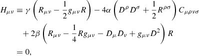 (2)
(2)
where Dμ is the covariant derivative and the symbol Hμν is introduced for convenience. Matter degrees of freedom can be included by adding the standard stress–energy tensor to the right-hand side of this equation. As our work focuses on vacuum solutions, we do not consider this extension. Invariance of the action (1) under general coordinate transformations ensures the generalized conservation law
 (3)
(3)
Furthermore, taking the trace of (2) gives
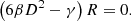 (4)
(4)
For β = 0, this latter relation implies R = 0, stating that vacuum solutions of Einstein-Weyl gravity must have a vanishing Ricci scalar. In the presence of the R2 coupling, this condition is not necessarily true and more general solutions are admissible.
We are interested in the static, spherically symmetric solutions of the system (2). The most general spacetime metric compatible with these requirements can be cast into the form (Hawking & Ellis 2011)
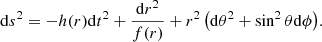 (5)
(5)
The Schwarzschild metric is given by
 (6)
(6)
where M is the ADM mass of the black hole according to Arnowitt, Deser, and Misner (Arnowitt et al. 1959).
In order to determine the functions h(r) and f(r), we substitute the ansatz (5) into the general equations of motion (2). This leads to a set of coupled, nonlinear differential equations. Of those, only two are independent. We select
 (7)
(7)
The angular equations are then fulfilled due to the constraint in Eq. (3). In the following, we focus on the generic case where α ≠ 0, α ≠ 3β, and β ≠ 0. In order to illustrate the differential order of the system (7), we follow Lü et al. (2015a). We first observe that the highest order derivatives appearing in Htt are f(3)(r) and h(4)(r), while Hrr depends on f(2)(r) and h(3)(r). We then define the auxiliary functions
![Mathematical equation: $$ \begin{aligned}&X(r) = \frac{h (\alpha - 3 \beta )}{\left(r (\alpha -3 \beta ) h^\prime -2 h (\alpha + 6 \beta )\right)^2}\nonumber \\&\qquad \quad \times \left[2 h r f^\prime \left(2 h (\alpha +6 \beta ) -r (\alpha -3 \beta ) h^\prime \right)\right.\nonumber \\&\qquad \quad \left. +f \left(12 h^2 (\alpha +6 \beta )-r^2 (\alpha -3 \beta ) (h^\prime )^2-4 h h^\prime r (\alpha -3 \beta )\right)\right]\end{aligned} $$](/articles/aa/full_html/2023/05/aa44080-22/aa44080-22-eq8.gif) (8)
(8)
 (9)
(9)
and introduce the new equations
 (10)
(10)
Clearly, the equations of motion (7) are equivalent to
 (11)
(11)
that is, we have rewritten the previous equations of motion into an equivalent form that is tailored to demonstrating the order of the system. The first equation is of second order in f and third order in h while the second equation is of third order in f and second order in h. Thus, taking the linear combination (10) has reduced the differential order of the vacuum equation by one, which is remarkable because one generally expects fourth-order derivatives on f and h in a theory that is quadratic in curvature. In the present case, locally, solutions of the system (11) are expected to be parameterized by six free parameters.
2.2. Local properties of the solutions
In order to construct the solutions of (11), we start by investigating the admissible asymptotic behaviors for large and small values of r.
2.2.1. Asymptotic flatness
Let us start by analyzing the structure of the solutions for large values of r. In this regime, gravity is expected to be weak. Thus, the asymptotics of the solutions can be obtained analytically by solving the linearized equations of motion obtained by perturbing the metric around flat Minkowski space. Following Bonanno & Silveravalle (2021), this procedure is implemented by writing
 (12)
(12)
Substituting this expression into the nonlinear equations (11) and expanding to first order in ϵ then yields
 (13)
(13)
This system is readily solved using Fourier methods. Introducing the masses of the massive spin-two and spin-zero degrees of freedom,
 (14)
(14)
we obtain, at linear order,
 (15)
(15)
Imposing the condition that the masses m0 and m2 are real restricts the values of the coupling constants to α ≥ 0, β ≥ 0. This choice ensures the absence of oscillating factors in the linearized solution, which are incompatible with asymptotic flatness. It is natural to expect the masses to be much smaller than those of astrophysical black holes. The canonical normalization of the time-coordinate and asymptotic flatness fix the parameters CT = 0 and  , respectively. Thus, for fixed α, β, asymptotically flat solutions comprise a three-dimensional solution space spanned by
  :
:
 (16)
(16)
This expression admits a simple particle physics interpretation: for  , the result for h(r) and f(r) agrees with the Schwarzschild solution. This part is governed by the massless degrees of freedom encoded in general relativity. The quadratic curvature terms lead to Yukawa-type corrections whose fall-off behavior at large distances is controlled by the spin-two mass m2 and spin-zero mass m0, respectively. The corrections to the Schwarzschild metric therefore decrease exponentially as r → ∞, and it is for this reason that they escape the classification with the standard Frobenius method (Saueressig et al. 2021).
For α = 0, β ≠ 0 and β = 0, α ≠ 0, the action integrand (1) reduces to the form R + R2 and R + CμνρσCμνρσ, respectively. From (14), we observe that in these limits the masses diverge, m2 → ∞ and m0 → ∞, respectively, and the corresponding massive degrees of freedom decouple. At the level of (16), this entails that the space of asymptotically flat solutions is spanned by only two free parameters, as either  or
or  drop out of the linearized solution. This can also be inferred from (13), where setting either α = 0 or β = 0 reduces the order of the linearized equations. We also note that the equal mass limit m0 = m2 (corresponding to the special case β = α/3) does not reduce the dimension of the solution space, because the free parameters
  and
and  enter into h(r) and f(r) in the form of two different linear combinations. Below, based on these insights, we analyze the space of vacuum solutions for the generic situation where α ≠ 0 and β ≠ 0.
2.2.2. Admissible scaling behavior for small r
Upon constructing the solutions of the linearized system of equations, we now determine the admissible scaling behaviors as r → 0. Later on, this will serve as a cross-check of the validity of our numerical solutions. We then write h(r) and f(r) as a power series in r, which is referred to as a Frobenius ansatz1:
 (17)
(17)
Here, h0 ≠ 0 and f0 ≠ 0 by definition and the exponents (s, t) capture the short-scale behavior of the solution. We then substitute the expansion (17) into the system of nonlinear equations (11) and determine the admissible values for s and t by analyzing the equations appearing at leading order at r = 0. The consistent values are referred to as analytic classes (s, t)0 where the subscript ‘0’ indicates that the expansion point is r = 0. In this way, we confirm the three solutions covered by Stelle (1977) and Lü et al. (2015a), which we tabulate in the upper half of Table 1. Going to higher powers of r and solving the corresponding equations recursively for the highest coefficients hn, fn contained in them allows us to fix the power series in terms of a set of undetermined coefficients. For the admissible scaling behaviors, the number and choice of free coefficients is then listed in Cols. 4 and 5 of Table 1. Moreover, the scaling behaviors allow us to determine the strength of the curvature singularity by evaluating the Kretschmann scalar RμνρσRμνρσ in the limit r → 0. The results are listed in the sixth column of Table 1, indicating that the naked singularity solutions are more divergent than the Schwarzschild solution.
At this stage, two technical remarks are in order. Firstly, the ansatz (17) covers solutions that have a series expansion at r = 0 only. Solutions that are not analytic at the expansion point would be missed by the scaling classification. Our numerical investigation did not provide evidence for the presence of such solutions, but all of our solutions comply with the scaling behaviors listed in Table 1. Secondly, one still has the freedom of rescaling the time coordinate by an arbitrary constant coefficient. This freedom could, in principle, be used to eliminate h0 from the list of free parameters. However, when constructing global solutions, we used this freedom to impose asymptotic flatness, and so this parameter is kept as a free parameter.
2.2.3. Admissible scaling behavior around a finite radius r0
There are also spacetime solutions in which the asymptotic form of the metric at infinity does not allow a smooth continuation to r = 0. These cases can be investigated by a Frobenius expansion at a finite radial coordinate r0. Similarly to the ansatz (17), one performs a formal power-series ansatz with integer values n:
 (18)
(18)
The possibility of having more general scaling laws including half-integer values for n was discussed by Lü et al. (2015a) but does not play a role in the following. Substituting the ansatz into the nonlinear equations of motion, the admissible values (s, t)r0 and the series coefficients  and
and  (apart from the free parameters spanning the solution space) can be obtained by solving the resulting hierarchy of equations iteratively. The incidental polynomials, appearing at lowest order in this expansion, admit infinite families of solutions:
 (19)
(19)
A specific selection from these solutions, classified by the labels (s, t)r0, is given in the lower half of Table 1. The expansion at a regular point, where both h(r0) and f(r0) are finite, is covered by (s, t)r0 = (0, 0)r0. The horizon appearing in the Schwarzschild solution is encoded in the (s, t)r0 = (1, 1)r0 class. Moreover, we encounter the class (1, 0)r0, in which f(r) vanishes linearly at r0 while h(r) stays finite. These solutions can be associated with wormhole solutions (Lü et al. 2015a).
2.3. Constructing the phase space
Equation (16) gives the parametrization of asymptotically flat solutions in the linearized regime. Fixing γ = 1/G = 1, which states that all dimensionful quantities are measured in Planck units, the solution space is spanned by five parameters: α, β, M,  , and
, and  . Evaluating the expression at ri > 3M then gives initial conditions for the nonlinear equations of motion from which the solution can be integrated inward numerically.
We note that the process of extending the solutions to r > ri is computationally difficult for the following reason. At the linearized level, asymptotically flat solutions span a subspace of the full solution space (15). The additional modes excluded by the asymptotic flatness condition grow exponentially as r increases. This makes the integration procedure unstable: tiny numerical errors can turn on the unstable perturbations, which then grow and drive the solution away from asymptotic flatness. It is clear that this is a technical and not a conceptual problem. Equation (16) guarantees that the asymptotically flat solutions extend to r → ∞. Placing initial conditions further away from the center, it is then simply a question of computational power to extend these conditions inward. Practically, we then chose initial conditions at ri = 3.5M, which we found to be a good working compromise between being in a regime where the Schwarzschild solution is a good approximation and having exponential corrections that remain at a value that can be handled numerically.
By varying the parameters systematically, we identify a number of topologically distinct solutions that can be discriminated according to their scaling behavior close to r = 0 (or their termination point rterm > 0, if applicable). The characteristic features of the resulting classes (Type I, II, and III) are then described below. This discussion is complemented by the representative examples shown in Figs. 1 and 2 arising from the initial conditions listed in Table 2. Following Hernandéz-Lorenzo & Steinwachs (2020), the scaling exponents are found by fitting to the global solutions in the vicinity close to the end point. This procedure introduces a numerical uncertainty. In the case of Type I solutions, the fit is almost perfect with a deviation of less than order 10−3. For Type II and Type III solutions, we commonly observe deviations of approximately 5%. For some Type III examples, such deviations may even increase to 50% in some extreme cases.
 |
Fig. 1. Illustration of the topologically distinct global solutions in quadratic gravity. The solutions are obtained from solving (11) numerically with initial conditions given in Table 2. The top line displays the radial dependence of lnf (blue curve) and lnh (orange curve) for the solutions of (a) Type I, (b) Type II, and (c) Type III. The Schwarzschild solution with M = 10 and an event horizon at r/M = 2 is superimposed as the dashed line. The lower row shows the scaling behavior of the solutions as r → 0 (Type I and Type II) as well as for r − r0 → 0 (Type III) in a double logarithmic presentation. The scaling behaviors are (s, t)0 = ( − 2, 2)0 for Type I, (s, t)0 = ( − 1, −1)0 for Type II, and (s, t)r0 = (1, 0)r0 for Type III. Graphs of the respective power law are superimposed as dashed lines (black for h and orange for f). This links the asymptotically flat, global solutions to the classification of local scaling behaviors identified in Table 1. |
 |
Fig. 2. Refinement of the Type-I classification. The solutions arise from the initial conditions given in Table 2 for objects of mass M = 10. The left panel displays lnf (top, solid) and lnh (bottom, dashed), showing the typical behavior of the Type I solutions given in Fig. 1a. The refinement follows from considering Veff = h(r)/r2, shown in the right panel. For Type Ia solutions, Veff decreases monotonically for r < 3M. For Type Ib solutions, the potential has a stable minimum and Veff(0) < Veff(3M). The characteristic feature for Type Ic solutions is that ∞ > Veff(0) > Veff(3M). |
Initial conditions for the numerical integration procedure generating the representative geometry for each class.
Type I. For these solutions the numerical integration is reliable until r ≈ 0. For r ≳ 2M, the functions h(r) and f(r) essentially follow the Schwarzschild solution, before starting to deviate substantially for r ≲ 2M. At r ≪ 1, the scaling behavior of h(r) and f(r) follows the local expansion with (s, t)0 = ( − 2, 2)0, that is,
 (20)
(20)
where the tilde indicates that the relations hold asymptotically. This constitutes the defining criterion for geometries of Type I. A characteristic example for these solutions is shown in Fig. 1a.
The effective radial potential governing the motion of light rays within the geometry is given by Veff(r) = h(r)/r2 (see Eq. (39) below). The scaling properties (20) then imply that Veff|r = 0 is finite. This suggests a refined classification based on the value h0, controlling the height of Veff at r = 0. From the perspective of observations, it is natural to discriminate the three subclasses displayed in Fig. 2:
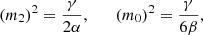
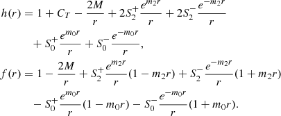
Type II. Similarly to Type I, the numerical integration of this class of solutions is reliable up to very small values r ≈ 0. Again the functions h and f follow the Schwarzschild solution for r > 2M and deviate for r ≤ 2M. The defining property of this class is its characteristic scaling behavior as r → 0,
 (21)
(21)
These solutions therefore belong to the analytic class ( − 1, −1)0, which describes naked singularities (Lü et al. 2015a). An example solution is illustrated in Fig. 1b. In the phase space plot in Fig. 3, Type II is indicated in yellow.
 |
Fig. 3. Several representative β-slices through the phase space. The values for |


Type III. The numerical integration for this solution class terminates at a radius rterm > 2M, at radii slightly larger than the position of the would-be horizon of a Schwarzschild black hole with equal asymptotic mass. Close to the termination point,
 (22)
(22)
meaning that these geometries fall into the analytic class (1, 0)r0. This corresponds to wormhole solutions (Lü et al. 2015a). An example Type III solution is illustrated in Fig. 1c. In the phase space plot in Fig. 3, Type III is indicated in black.
Now that we have a complete classification of the individual phase-space elements, we now proceed to construct the phase space of static, asymptotically flat, and spherically symmetric vacuum solutions in quadratic gravity. As the solution space is spanned by five free parameters, we reduce the complexity of the problem by fixing the asymptotic mass of the solutions, M = 10 in natural units2, and the mass of the massive spin-two degree of freedom, m2 = 1 (equivalently, α = 1/2). As M is accessible via observations in the weak-gravity regime, it is natural to keep this variable fixed while analyzing the solution space. At the same time, keeping α fixed and varying β allows us to investigate the relative impact of the quadratic gravity contributions associated with the massive spin-two and spin-zero degrees of freedom. The remaining three parameters, β,  , and
, and  , are varied to construct representative two-dimensional slices of the phase space. For our purposes, β takes the values (1/3, 1/4, 1/5, 1/6, 13/84, 1/7, 1/8, 1/10, 1/18). For each value of β, we investigate all combinations of the Yukawa amplitudes
  and
and  , taking values in (±10, ±5, ±2, ±1, ±0.5, ±0.2, ±0.1, ±0.05, ±0.02, ±0.01, ±0.005, ±0.002, ±0.001, 0). In total, this results in approximately 104 spacetime geometries.
We then use (16) to impose initial conditions at ri = 3.5M and integrate inwards, identifying the corresponding solution class by matching the numerical result to the analytic scaling behavior close to the termination point. The distribution of the numeric solution classes is visualized in Fig. 3 with the color code in Table 3. This clearly illustrates that quadratic gravity admits a rich phase space of black-hole-type solutions. Notably, the Schwarzschild solution appears for all values α, β and is situated at  ; it constitutes the only solution with an event horizon. This is in agreement with the expectation that there is no infinitesimal deformation of Schwarzschild in the context of quadratic gravity that allows a smooth transition to another solution class (Lü et al. 2015a).
Mapping numeric solution classes to analytic classes.
At this point it is worth highlighting several features of our result. Let us start with the case β = 1/6, which corresponds to the spin-zero and spin-two mass being equal, m2 = m0 = 1. Here, both Yukawa potentials show the same damping and we can realize all types of geometries by dialing  and
and  . Decreasing β leads to an increase in m0. This results in a relative suppression of the spin-zero contributions with respect to those of spin-two. As a consequence, the initial conditions become almost independent of
  , which means that the lines separating different phases turn vertically (cf. the subfigure for β = 1/3). Conversely, increasing β beyond the equal-mass case leads to a relative suppression of the spin-two contribution and the phase space becomes mostly independent of
  . This effect underlies the horizontal stripes obtained at β = 1/18.
We checked the robustness of the phase space classification shown in Fig. 3 by varying the value ri where the initial conditions are imposed. While this results in minor changes in the functions h(r) and f(r), the analytic scaling class of the solutions remains largely unaffected. The small number of cases where the change of ri actually triggers a change in the classification are indicated as white squares. Notably, these appear close to a phase transition line, indicating that our numerical construction is not sufficiently elaborate to associate the point to a specific phase.
An intriguing consequence of the phase space shown in Fig. 3 is that it is actually quite difficult to discriminate general relativity and quadratic gravity based on its static, spherically symmetric, and asymptotically flat solutions. As the Schwarzschild geometry solves both equations of motion, any experiment confirming the validity of this solution can be understood as an experimental verification of both theories. Distinguishing among the two settings is possible if, and only if, an experiment actually detects a deviation from the GR, which could then point towards an alternative geometry appearing in the phase space of quadratic gravity.
Notably, the stability of spacetimes with potentials similar to the ones encountered for the solutions Type Ic and Type II (and potentially also Type Ib) has been discussed in the context of ultracompact objects by Cardoso et al. (2014) and Keir (2016). In this context, it was argued that gravitational wave perturbations could potentially destabilize the geometry. We defer a detailed discussion of such an effect on our geometries to future work.
3. Constraining quadratic gravity through its shadow
In the previous section, we demonstrate that the phase space of static, spherically symmetric, and asymptotically flat solutions appearing in quadratic gravity comes with two sets of free parameters. Firstly, the masses m2 and m0 introduced in Eq. (14) are directly related to the coupling constants associated with the higher derivative interactions. Secondly, the parameters  , with M being the asymptotic mass of the solution, parameterize the solution space for fixed masses (m2, m0). In order to constrain the additional parameters for quadratic gravity through observations, we systematically compute observables from the underlying geometries. As the solutions spanning the phase space are virtually degenerate far away from the gravitational source, the focus is on the strong gravity regime situated within the unstable photon orbit of the geometries. Practically, we limit ourselves to observables, which are accessible by the EHT. The coordinate radius of the outer (unstable) photon orbit is considered in Sect. 3.1. Here we demonstrate that this observable turns out to be virtually identical for the Schwarzschild solution and the geometries associated with naked singularities. Following Bambi (2013) and Shaikh et al. (2019), we then consider the intensity profile of light geodesics originating from radially free-falling, spherically symmetric accreting matter around the gravitational source. Throughout this section, we work in the probe approximation, neglecting matter self-interactions as well as the backreaction of the matter on the geometry.
3.1. Photon rings
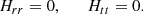
Making the implicit assumption that the radius separating the plunge rays from the rays going out to infinity coincides with the position of the unstable photon sphere, Psaltis et al. (2020) derived that, for spherically symmetric spacetimes, the coordinate radius rsh of the shadow measured by a distant observer depends on the tt-component of the metric. Based on the areal coordinate system used in (5), one finds
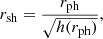 (23)
(23)
where rph is the coordinate radius of the unstable photon orbit, determined from the condition
 (24)
(24)
The angular radius of the photon ring on the sky is then given by θph = rph/D with D the distance to the object. In practise, observations give θph = 42 ± 3 μas (The Event Horizon Telescope Collaboration 2019a).
For the Schwarzschild case (6), one recovers rph = 3M and the coordinate radius of the shadow equates to
 (25)
(25)
We introduce
 (26)
(26)
to measure the deviation of the shadow position as compared to the Schwarzschild case.
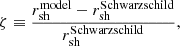
We now turn our attention to the photon ring radius – assuming the linearized solution in (16) still holds – with the aim being to evaluate the deviation parameter ζ for the astrophysical black hole M 87* in mind. Evaluating Eq. (24) for the linearized solution, we obtain, in linear approximation,
 (27)
(27)
For this formula to be valid, one needs the condition 3 mi M ≫ 1 to be satisfied for both relevant masses m0, m2. If the linearized solution is valid near the photon ring, it is also valid outside of it and therefore the linearized solution can also be plugged into Eq. (23) to obtain rsh. Setting, for simplicity,  (or equivalently, for the purposes here, taking β = 0), we have for the shadow radius
 (28)
(28)
We note that, generally, the smaller m2, the bigger the deviation of the shadow radius is compared to the Schwarzschild case. Assuming m2 to be of the order of the Planck mass, say m2 = mpl, and taking M = 2.2 × 1050 mpl as roughly the mass of the black hole M 87*, for the deviation parameter we get
 (29)
(29)
Clearly, for any seemingly realistic values of  , this number is zero for all practical purposes. This serves as a typical example of how small quantum gravity corrections can be, and serves as a direct demonstration that the modifications of the quadratic gravity terms do not (significantly) extend to the photon radius. However, as the modifications do extend to just beyond the would-be horizon, we now discuss another observable that can be seriously affected by the solutions presented in Sect. 2.
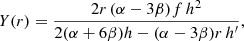
3.2. Intensity profiles from accreting matter
A second observable related to observations by the EHT is the intensity profile of radiation emitted by surrounding matter. In this work, we study this observable based on the optically thin accreting matter model proposed by Bambi (2013). This model has already been used to compare the intensity profiles of a Schwarzschild black hole and a wormhole geometry (Bambi 2013), and subsequently Schwarzschild black holes and naked singularities given by the Joshi-Malafarina-Narayan spacetimes (Shaikh et al. 2019; Kaur et al. 2021), showing that the difference in geometry leads to distinguished features in the intensity profile. The key advantage of this model is that it is sufficiently simple that the intensity profiles can be obtained without numerically expensive ray-tracing techniques. In this way, one can actually evaluate the profiles for a large number of geometries comprising the phase space discussed in Sect. 2.33.
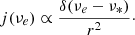
The matter, accreting to the center of gravity, is taken to be spherically symmetric, optically thin, and radially free-falling; it emits monochromatic radiation whose emissivity in the emitter frame per unit volume falls proportional to r−2; see also Falcke et al. (2000):
 (30)
(30)
Here, ν* is the emitted photon frequency in the rest frame of the emitter. We are then interested in the intensity of light detected by an observer at rest situated at a distance D ≫ M from the black hole. Introducing X, Y as the coordinates on the screen of the asymptotic observer, the intensity of photons observed at frequency νobs is given by (Jaroszynski & Kurpiewski 1997)
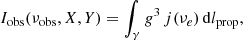 (31)
(31)
where γ denotes the path taken by the photon, g = νobs/νe is the redshift factor, and dlprop is the infinitesimal proper length measured in the rest frame of the emitter. These can be expressed in terms of the 4-momentum of the photon kμ, the 4-velocity of the observer 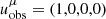 , and the 4-velocity of the accreting matter
  . Starting from (5), and considering a spherically symmetric gas in radial free-fall, the latter is given by
 (32)
(32)
For a photon, the t-component of the 4-momentum kμ is a constant of integration. For radial motion, the r-component can then be obtained from the fact that kμ is light-like, satisfying kμkμ = 0. Using the Euler-Lagrange equations to infer that kt = E and kϕ = L are constants of motion, one has
 (33)
(33)
with b2 ≡ L2/E2 being the impact parameter of the ray. The +(−) sign holds when the photon approaches (moves away from) the center of gravity. The redshift factor is given by
 (34)
(34)
Substituting the explicit expressions for the 4-velocities together with (33) gives
 (35)
(35)
where the sign again refers to photons moving towards (or away from) the center of gravity. Finally, the proper distance  can be evaluated in terms of the 4-momentum of the photon and the redshift factor
 (36)
(36)
Substituting these intermediate results into Eq. (31) and integrating over all frequencies finally gives (Bambi 2013)
 (37)
(37)
For an observer sufficiently far away from the center of gravity, X2 + Y2 = b2 and the right-hand side of (37) depends on the impact parameter b only. Owing to the spherical symmetry of the model, it is then sufficient to calculate the intensity as a function of b only.
In practice, we construct the intensity profiles as follows. The screen, corresponding to the telescope situated far away from the gravitational source, is placed at a coordinate distance ds = 105M away from the center of gravity. Starting from the screen, the light rays are then traced backwards through spacetime. Owing to the spherical symmetry of the geometry, it is sufficient to trace rays within the equatorial plane θ = π/2. For these paths,
 (38)
(38)
are integrals of motion. This allows us to convert the condition for light-like geodesics,  , into a first-order equation determining r(s):
 (39)
(39)
where Veff(r)≡h(r)/r2. Based on the explicit value for b, one distinguishes two types of light rays. If  at some radius r, the photon trajectory γ has a turning point there and continues outward towards infinity. In this case, the total intensity picked up along the ray consists of two contributions: for the part of γ connecting the screen to the turning point, Eq. (37) is evaluated choosing the minus sign in (35) while the intensity picked up on the other side of the turning point is given by (37) evaluated with the redshift factor for photons going towards the source. The observed intensity is then given by the sum of these contributions. The second class of light rays does not possess a turning point and therefore goes on until it reaches a termination point. For the Schwarzschild geometry, the rays terminate at the event horizon, while for geometries of Type I the rays reach r = 0 where they hit the curvature singularity. Now, r(s) decreases monotonically and the intensity formula is integrated from the termination point of the object to the screen using the minus sign in (35).
At this stage, several important remarks on evaluating (37) are in order. For r > 3M, all our example geometries agree with the Schwarzschild geometry up to exponentially suppressed correction terms. This feature entails that light rays not entering the region r < 3M see the same geometry irrespective of the solution. The tail of the intensity profiles where b > bcrit is universal and shared by all geometries: this part of the profile only probes spacetime in regions where the quadratic gravity effects are negligible. The evaluation can therefore be sped up by simply focusing on light rays with b < bcrit and completing the intensity profile with the Schwarzschild result for b > bcrit. Secondly, this feature negates the need to extend the numerically constructed solutions up to the observer screen, which, owing to the instability of the equations, would result in an insurmountable fine-tuning problem for the initial conditions. Instead, the outer region of spacetime can simply be taken to be the Schwarzschild solution with the gluing point taken at r = 3M. Finally, evaluating the intensity profile for wormhole geometries (Type III) requires additional assumptions. In this case, f(rt) = 0 at a finite value rt > 2M and the geometry can be extended to r < rt in such a way that rt describes the throat of the wormhole. We then adopt the assumption made by Bambi (2013) that no radiation comes out of the hole. The intensity picked up along rays connecting to the throat is therefore obtained by integrating (37) from rt to the screen.
The characteristic intensity profiles – as a function of the ray’s impact parameter b – associated with the geometries generated from the initial conditions in Table 2 are shown in Fig. 4. The reference profile obtained from the Schwarzschild geometry is depicted in the left column. In this case, the intensity shows a step rise at  , marking the impact parameter for which the ray touches the unstable photon orbit. For b < bcrit, the rays plunge into the black hole horizon, creating the low-intensity region associated with the black hole shadow shown in the bottom-left panel of Fig. 4. The intensity profiles resulting from the geometries of Type Ia, Type Ib, and Type III are indistinguishable from the reference plot and are therefore not shown separately. Therefore, despite the region 0 < r < 2M contributing to the intensity profiles of Type Ia and Type Ib, this contribution is found to be negligible4. Similarly, the regions where the Type III geometry differs from the Schwarzschild reference also make negligible contributions to the intensity profile.
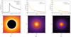 |
Fig. 4. Distinguished intensity profiles for spacetimes obtained from the initial conditions listed in Table 2 assuming the emission model (37). The left column shows the intensity for a Schwarzschild black hole with M = 10 (top row). This intensity profile is virtually indistinguishable from naked singularities of Type Ia, Type Ib, and Type III. The middle column gives the intensity for the Type Ic solution with initial conditions. The size of the shadow of a Schwarzschild black hole is added as a dashed line for reference. The presence of an inner turning point significantly enhances the intensity in the region btp2 ≤ b ≤ bcrit. Intensity profiles for Type II solutions illustrated in the right column do not exhibit a shadow; their image resembles that of a star with the peak intensity at small impact parameter b. |
The intensity profile generated by geometries of Type Ic is shown in the middle column of Fig. 4. These geometries again exhibit a shadow region, albeit with smaller radius bType − Ic − shadow < bcrit. This effect is shown in the bottom central panel of Fig. 4 where the shadow size of the Schwarzschild black hole with identical asymptotic mass is superimposed as the white dashed circle. The interval bType − Ic − shadow < b < bcrit is indeed brighter than the intensity found in the tail at b > bcrit. This is a direct consequence of the characteristic property of Type Ic geometries where Veff|r = 0 > Veff|r = 3M by definition; see Fig. 2. Owing to this property, light rays entering the region r < 3M can still exhibit a turning point and be reflected back to asymptotic infinity. Depending on the actual value of Veff|r = 0, this leads to a significant gain of intensity for b < bcrit. This effect can be used to rule out part of the Type Ic solution space based on shadow observations.
Finally, we exemplify the intensity profile associated with geometries of Type II in the right column of Fig. 4. In this case, Veff|r = 0 = ∞ and all light rays with b > 0 have a turning point and go out to asymptotic infinity. As a consequence, these geometries do not cast a shadow. Their profile resembles that of a star where the maximum intensity is reached in the center of the image. Based on this distinguished feature, Type II geometries are ruled out observationally.
Heuristically, the enhanced brightness in the case of Type Ic and Type II solutions can be understood as follows. For all types of solutions, once a ray is inside the unstable photon region and is headed towards the interior, the light ray will continue to head inwards and eventually approaches the singularity. For solutions of Type Ia or Ib (and similarly for Type III solutions), the light rays inevitably reach the singularity and terminate there. However, for Type II solutions, the light rays are reflected near the singularity due to the infinitely high potential barrier that is present at the center. The rays then extend outward to infinity again, following the mirrored trajectory but now in the opposite direction; see Fig. 5. Due to this reflection, the intensity picked up by the ray is significantly enhanced for two reasons. First, the ray crosses the region where light is emitted twice, leading to an increase in the intensity. Secondly, light rays that first go towards the interior, are reflected, and then go out and reach the observer at infinity are first blueshifted and then redshifted. The rather severe redshift effect obtained by climbing out of the interior is compensated by first falling inwards, negating its effect. For Type Ic solutions, only rays with an impact parameter above some critical value – determined by the height of the potential barrier – are reflected, and therefore still leave a (smaller) shadow.
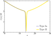 |
Fig. 5. Radius r(s) plotted as a function of the path parameter s, with an impact parameter of b/M = 0.05 for an object of mass M = 10. For the geometry of Type Ia, the ray terminates at the singularity, while for the Type II geometry the light ray is reflected instead. This feature where the trajectory is extended, going back out to infinity again, is the underlying reason for why the brightness in the interior is enhanced for Type II and Type Ic solutions, as can be seen in Fig. 4. |
We point out that the unstable photon orbit imprints a peak at bcrit in the intensity profiles (Fig. 4). As the critical impact parameter agrees with the Schwarzschild value almost exactly, that peak position contains important information: the asymptotic mass of the object. For geometries of Type Ic and Type II, the peak provides an intrinsic scale in the image.
We complete our discussion by giving the relative strength of a signal distinguishing the Schwarzschild solution from alternatives. We define the relative difference in the intensity profiles as
 (40)
(40)
Figure 6 then shows η as a function of the impact parameter for all examples introduced in Table 2. For geometries of Type Ia, Type Ib, and Type III shown in the left panel, η ≪ 1 and is of the order of the numerical integration accuracy. We therefore do not give details for these cases. The associated regions in the quadratic gravity phase space, shaded in pink, red, and black in Fig. 3, are not excluded by black hole shadow observations consistent with the GR prediction. In contrast, the geometries of Type Ic and Type II exhibit distinguished and pronounced differences in the intensity profiles. For Type Ic, the size of the shadow depends on the specific parameter values, in particular on α, β,  , and
, and  , and therefore the associated region in phase space can be constrained by more refined black hole shadow observations. For Type II, we find η ≈ 𝒪(10) in the interior. The enhancement of the intensity toward the center of the image is a topological effect valid for all parameter combinations, in contrast to an intensity depression in the Schwarzschild case. This signature is sufficiently pronounced to completely rule out Type II as an alternative to the Schwarzschild black hole based on shadow observations (The Event Horizon Telescope Collaboration 2019a). Therefore, at the level of Fig. 3, parts of the phase space shaded in orange can be restricted while yellow-shaded areas are not compatible with observations.
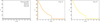 |
Fig. 6. Relative intensity difference from the Schwarzschild black hole, as defined in Eq. (40), for a mass parameter M = 10. Left: Type Ia, Ib, III. Center: Type Ic. Right: Type II solution. The latter two cases show distinguished and strong deviations from the Schwarzschild case, which allow us to distinguish between the geometries based on shadow images. |
4. Summary and outlook
4.1. Main results
This work focuses on quadratic gravity, and its implications for images made by the EHT. The strategy employed here was to first restrict our scope to vacuum solutions that are static, spherically symmetric, and asymptotically flat. We then looked at the asymptotic behavior of these solutions by solving the linearized equations of motion of quadratic gravity. This shows that, at fixed Newton’s coupling, there is a five-dimensional space of asymptotically flat geometries parameterized by the two additional coupling constants of the theory and three parameters spanning the solution space at fixed values of the couplings. The latter can be associated with the asymptotic mass M of the solution and the strengths of the (exponentially suppressed) Yukawa-type interactions introduced by the additional massive degrees of freedom of the theory. The linearized solutions provide initial conditions for integrating the full nonlinear equations of motion numerically, thereby obtaining global geometries. As their key feature, the global geometries track the Schwarzschild solutions almost perfectly for r ≳ 2M while deviating substantially within the would-be event horizon5. The solutions are in agreement with the local scaling behaviors determined analytically by the Frobenius method. Our scan of the phase space, comprising around 104 geometries, identified the following types of solutions. First, we recovered the Schwarzschild spacetime familiar from general relativity which is also a solution to quadratic gravity. Secondly, we identified naked singularities of Type I (coming in subclasses a,b,c) and Type II. Thirdly, we encountered wormhole solutions, which are classified as Type III geometries. All solutions are compatible with the local scaling behaviors identified earlier by Lü et al. (2015a) and Holdom (2002). Conversely, not all local scaling behaviors arising from the Frobenius analysis are realized by extending asymptotically flat solutions. Our work, for the first time, combines these results in a comprehensive picture on the phase space of static, spherically symmetric, and asymptotically flat vacuum solutions in quadratic gravity.
Our numerical investigation also supports the argument given by Lü et al. (2015a) that, for α ≠ 0, β ≠ 0, the Schwarzschild solution is the only geometry within the phase space exhibiting an event horizon. While it is known that the Stelle black hole provides an additional black hole geometry with a horizon (Lü et al. 2015b), this does not appear in our phase space construction because our choice of M is above the critical mass for which this branch of solutions exists. Thus, our analysis suggests the following Birkhoff-type uniqueness theorem for sufficiently massive black holes: the only static, spherically symmetric, and asymptotically flat solution of (generic) quadratic gravity compatible with the cosmic censorship hypothesis is the Schwarzschild solution.
Subsequently, we addressed the question of whether images taken by the EHT can be used to discriminate between the various types of geometries encountered in the phase space of quadratic gravity. In this context, the first observation made by our work is that all geometries constructed in Sect. 2 are essentially identical at coordinate distances r ≳ 2M with significant deviations appearing close to and below r = 2M only. In particular, the location of the unstable photon orbit setting the size of the shadow cast by the Schwarzschild geometry is identical up to exponentially small corrections. The location of this orbit does not therefore allow us to discriminate between the geometries.
Moreover, we equipped our geometries with the simple emission model proposed by Bambi (2013)6. We show that the resulting intensity profiles allow us to easily distinguish the Schwarzschild geometry from geometries of Type Ic and Type II, as these geometries exhibit a significant increase in intensity within the shadow region of the Schwarzschild black hole with identical asymptotic mass (cf. Fig. 6). The relative distribution of the effect is easily resolvable by the EHT. For realistic masses, these geometries essentially agree with the Schwarzschild solution outside the event horizon, meaning that they cast identical shadows. Ultimately, this effect can be traced back to the fact that these geometries actually possess light-like geodesics with turning points at impact parameter b < bcrit where bcrit is the critical value separating the plunge orbits from rays going out to asymptotic infinity in the Schwarzschild geometry. This feature is absent for the geometries of Type Ia, Type Ib, and Type III. As a consequence, the intensity profiles obtained in these cases are identical to that of the Schwarzschild black hole for observational purposes.
These findings entail two important consequences. Firstly, the EHT has the capability of probing (and actually ruling out part of) the phase space of static, spherically symmetric, and asymptotically flat vacuum solutions in quadratic gravity. Secondly, this phase space contains horizonless, naked singularities and wormhole geometries whose intensity profiles are virtually indistinguishable from the ones created by the Schwarzschild geometry. On this basis alone, it is difficult to conclude whether or not the object imaged by the telescope actually possesses an event horizon.
4.2. Outlook
In this work, we established that observations by the EHT can be used to rule out parts of the phase space of quadratic gravity as alternatives to the black hole solutions found in general relativity. Clearly, the present work can be generalized in various directions.
Geometries including angular momentum. Realistic black holes are expected to carry angular momentum. This applies in particular to supermassive black holes in the center of galaxies. Although the inclusion of angular momentum has only a mild effect on the size and shape of the shadow cast by the black hole, slightly deforming the image asymmetrically, it would be highly interesting to generalize the geometries studied in the present work, relaxing the assumption of spherical symmetry.
More realistic intensity profiles. A more detailed comparison between theoretical predictions and actual observations will require more elaborate synthetic images of the shadow. We expect this to be achievable by improving the accretion disk model and applying advanced ray-tracing techniques developed by the EHT collaboration. The alternatives to the Schwarzschild geometry constructed in the present work may constitute theoretically well-motivated targets for such an investigation. In particular, it would be interesting to determine whether the improved emission model, potentially including outflows, allows us to discriminate between the Schwarzschild solution and a naked singularity of Type Ib, putting observational constraints on this part of phase space as well. This will be investigated in a a companion paper (Daas et al., in prep.).
Including quantum corrections. At this stage in our work we have constructed the vacuum solutions of classical quadratic gravity. As this theory is perturbatively renormalizable (Stelle 1977), it would be very interesting to study quantum corrections to the classical phase space by taking into account one-loop corrections to the action (1). Similarly, it would be interesting to understand how the two-loop counter-term found by Goroff & Sagnotti (1986) modifies the vacuum solutions of general relativity. As some of the intensity profiles constructed in our work actually probe spacetime in a regime where (quantum) gravity effects are expected to be strong, it is actually conceivable that there could be signatures of such terms contained in the observations.
Improving the image resolution. In comparison to the Schwarzschild solution, the shadow size of Type Ic geometries is decreased. Additionally, there is a ring-like brightness excess region appearing at the horizon position in the Schwarzschild case. This effect goes beyond a pure change of the shadow size; it also modifies the intensity profile. Depending on the parameters specifying the solution, both features can be more or less pronounced and might be limited to a small angular scale. Thus, they may be beyond the current effective resolution of the EHT, which amounts to ∼25 μas or roughly half of the ring diameter in the case of M 87* (The Event Horizon Telescope Collaboration 2019a). However, it might be feasible in the future, when extending the size of the Earth-sized telescope array into space using satellites, which will improve the EHT resolution by one order of magnitude or more (Roelofs et al. 2019). In addition, upcoming observations related to Sgr A* may provide further observational constraints.
Additional observables. Our present discussion focuses on discriminating geometries based on observation channels related to the EHT. In a similar spirit, Salvio (2022) aimed to constrain quadratic gravity based on early universe cosmology. Clearly, it would be interesting to complement these works by other observational channels related to, for example, the emission of gravitational waves. This may provide constraints that are complementary to the ones based on shadow observations, allowing us to further constrain deviations from general relativity motivated by fundamental quantum gravity considerations.
Frobenius expansions are in general applicable to linear differential equations. In our investigations we follow the literature which extends the usage to non-linear differential equations, see for instance Holdom (2002) and Lü et al. (2015a).
Irrespective of the concrete choice, the modifications of the solutions are of topological nature and therefore remain in an astrophysical setting.
For the proposal that the emission comes from the jet of astrophysical black holes, especially in the case of Sgr A* and M 87*, see Falcke et al. (1993) and Falcke & Markoff (2000). Accretion flows have been reviewed by Yuan & Narayan (2014).
For Type Ib, a more sophisticated emission model may bypass this conclusion because of the stable minimum exhibited by Veff. Detailed studies based on the RAPTOR ray-tracing code (Bronzwaer et al. 2018, 2020) are currently ongoing and will be reported elsewhere (Daas et al., in prep.).
A similar result based on renormalization group improvements in the context of the gravitational asymptotic safety program has recently been reported by Borissova et al. (2023).
This model was used to analyze intensity profiles related to phenomenologically motivated wormhole solutions by Bambi (2013). Later on, Shaikh et al. (2019) used the same model to construct characteristic intensity profiles associated with naked singularities of the JMN-1 and JMN-2 types. Depending on the model parameters, the resulting findings are in qualitative agreement with our results for Type I and Type II naked singularities.
Acknowledgments
We thank M. Bañados, A. Bonanno, T. Bronzwaer, and H. Olivares for interesting discussions and A. Khosravi and M. Galis for participating in the early stages of this investigation. Furthermore, we thank C. Bambi for correspondence on earlier work (Bambi 2013). This project was enabled by the Radboud Excellence fellowship awarded to M.F.W. by Radboud University in Nijmegen, The Netherlands. The work of F.S. is supported by the NWA-grant “The Dutch Black Hole Consortium”. While this work was under internal review, two preprints with content related to the solution classification appeared (Silveravalle 2022; Bonanno et al. 2022).
References
- Alvarez-Gaume, L., Kehagias, A., Kounnas, C., Lüst, D., & Riotto, A. 2016, Fortsch. Phys., 64, 176 [NASA ADS] [CrossRef] [Google Scholar]
- Arnowitt, R. L., Deser, S., & Misner, C. W. 1959, Phys. Rev., 116, 1322 [Google Scholar]
- Ashtekar, A., & Bojowald, M. 2006, Class. Quant. Grav., 23, 391 [NASA ADS] [CrossRef] [Google Scholar]
- Bambi, C. 2013, Phys. Rev. D, 87, 107501 [NASA ADS] [CrossRef] [Google Scholar]
- Bardeen, J. M. 1968, Proceedings of the International Conference GR5, Tbilisi, USSR, 174 [Google Scholar]
- Bern, Z., Cheung, C., Chi, H.-H., et al. 2015, Phys. Rev. Lett., 115, 211301 [NASA ADS] [CrossRef] [Google Scholar]
- Bonanno, A., & Reuter, M. 2000, Phys. Rev. D, 62, 043008 [Google Scholar]
- Bonanno, A., & Silveravalle, S. 2021, JCAP, 08, 050 [CrossRef] [Google Scholar]
- Bonanno, A., Khosravi, A.-P., & Saueressig, F. 2021, Phys. Rev. D, 103, 124027 [NASA ADS] [CrossRef] [Google Scholar]
- Bonanno, A., Silveravalle, S., & Zuccotti, A. 2022, Phys. Rev. D, 105, 124059 [NASA ADS] [CrossRef] [Google Scholar]
- Borissova, J. N., Held, A., & Afshordi, N. 2023, Class. Quantum Grav., 40, 075011 [NASA ADS] [CrossRef] [Google Scholar]
- Bronzwaer, T., & Falcke, H. 2021, ApJ, 920, 155 [NASA ADS] [CrossRef] [Google Scholar]
- Bronzwaer, T., Davelaar, J., Younsi, Z., et al. 2018, A&A, 613, A2 [NASA ADS] [CrossRef] [EDP Sciences] [Google Scholar]
- Bronzwaer, T., Younsi, Z., Davelaar, J., & Falcke, H. 2020, A&A, 641, A126 [NASA ADS] [CrossRef] [EDP Sciences] [Google Scholar]
- Camanho, X. O., Edelstein, J. D., Maldacena, J., & Zhiboedov, A. 2016, J. High Energy Phys., 02, 020 [CrossRef] [Google Scholar]
- Cardoso, V., Crispino, L. C. B., Macedo, C. F. B., Okawa, H., & Pani, P. 2014, Phys. Rev. D, 90, 044069 [Google Scholar]
- Deser, S., & Tekin, B. 2003, Phys. Rev. D, 67, 084009 [NASA ADS] [CrossRef] [Google Scholar]
- Donoghue, J. F. 1994, Phys. Rev. D, 50, 3874 [Google Scholar]
- Donoghue, J. F., Ivanov, M. M., & Shkerin, A. 2017, ArXiv e-prints [arXiv:1702.00319] [Google Scholar]
- Dymnikova, I. 1992, Gen. Relat. Grav., 24, 235 [CrossRef] [Google Scholar]
- Edelstein, J. D., Ghosh, R., Laddha, A., & Sarkar, S. 2021, J. High Energy Phys., 09, 150 [CrossRef] [Google Scholar]
- Eichhorn, A., & Held, A. 2021a, Eur. Phys. J. C, 81, 933 [NASA ADS] [CrossRef] [Google Scholar]
- Eichhorn, A., & Held, A. 2021b, JCAP, 05, 073 [CrossRef] [Google Scholar]
- Falcke, H., & Markoff, S. 2000, A&A, 362, 113 [NASA ADS] [Google Scholar]
- Falcke, H., Mannheim, K., & Biermann, P. L. 1993, A&A, 278, L1 [NASA ADS] [Google Scholar]
- Falcke, H., Melia, F., & Agol, E. 2000, ApJ, 528, L13 [Google Scholar]
- Frolov, V. P. 2016, Phys. Rev. D, 94, 104056 [NASA ADS] [CrossRef] [Google Scholar]
- Gambini, R., & Pullin, J. 2013, Phys. Rev. Lett., 110, 211301 [NASA ADS] [CrossRef] [Google Scholar]
- Gebhardt, K., Adams, J., Richstone, D., et al. 2011, ApJ, 729, 119 [Google Scholar]
- Ghosh, A., Jana, S., Mishra, A. K., & Sarkar, S. 2019, Phys. Rev. D, 100, 084054 [Google Scholar]
- Goroff, M. H., & Sagnotti, A. 1986, Nucl. Phys. B, 266, 709 [NASA ADS] [CrossRef] [Google Scholar]
- Hawking, S. W., & Ellis, G. F. R. 2011, The Large Scale Structure of Space-Time (Cambridge: Cambridge University Press) [Google Scholar]
- Hayward, S. A. 2006, Phys. Rev. Lett., 96, 031103 [CrossRef] [PubMed] [Google Scholar]
- Held, A., & Lim, H. 2021, Phys. Rev. D, 104, 084075 [NASA ADS] [CrossRef] [Google Scholar]
- Held, A., Gold, R., & Eichhorn, A. 2019, JCAP, 06, 029 [CrossRef] [Google Scholar]
- Hernandéz-Lorenzo, E., & Steinwachs, C. F. 2020, Phys. Rev. D, 101, 124046 [CrossRef] [Google Scholar]
- Holdom, B. 2002, Phys. Rev. D, 66, 084010 [Google Scholar]
- Jaroszynski, M., & Kurpiewski, A. 1997, A&A, 326, 419 [Google Scholar]
- Johannsen, T. 2013, Phys. Rev. D, 88, 044002 [NASA ADS] [CrossRef] [Google Scholar]
- Johannsen, T., & Psaltis, D. 2011, Phys. Rev. D, 83, 124015 [Google Scholar]
- Kaur, K. P., Joshi, P. S., Dey, D., Joshi, A. B., & Desai, R. P. 2021, ArXiv e-prints [arXiv:2106.13175] [Google Scholar]
- Keir, J. 2016, Class. Quant. Grav., 33, 135009 [NASA ADS] [CrossRef] [Google Scholar]
- Knorr, B., & Platania, A. 2022, Phys. Rev. D, 106, L021901 [NASA ADS] [CrossRef] [Google Scholar]
- Koch, B., & Saueressig, F. 2014, Int. J. Mod. Phys. A, 29, 1430011 [NASA ADS] [CrossRef] [Google Scholar]
- Kocherlakota, P., & Rezzolla, L. 2020, Phys. Rev. D, 102, 064058 [NASA ADS] [CrossRef] [Google Scholar]
- Konoplya, R., Rezzolla, L., & Zhidenko, A. 2016, Phys. Rev. D, 93, 064015 [Google Scholar]
- Kramer, M., Stairs, I. H., Manchester, R. N., et al. 2021, Phys. Rev. X, 11, 041050 [NASA ADS] [Google Scholar]
- LIGO Scientific Collaboration,& Virgo Collaboration (Abbott, B. P., et al.) 2016, Phys. Rev. Lett., 116, 061102 [CrossRef] [PubMed] [Google Scholar]
- Lü, H., Perkins, A., Pope, C. N., & Stelle, K. S. 2015a, Phys. Rev. D, 92, 124019 [CrossRef] [Google Scholar]
- Lü, H., Perkins, A., Pope, C. N., & Stelle, K. S. 2015b, Phys. Rev. Lett., 114, 171601 [CrossRef] [Google Scholar]
- Lü, H., Perkins, A., Pope, C. N., & Stelle, K. S. 2015c, Int. J. Mod. Phys. A, 30, 1545016 [CrossRef] [Google Scholar]
- Morales, J. O., & Santillán, O. P. 2019, JCAP, 03, 026 [CrossRef] [Google Scholar]
- Nicolini, P., Spallucci, E., & Wondrak, M. F. 2019, Phys. Lett. B, 797, 134888 [NASA ADS] [CrossRef] [Google Scholar]
- Noakes, D. R. 1983, J. Math. Phys., 24, 1846 [CrossRef] [Google Scholar]
- Percacci, R. 2017, An Introduction to Covariant Quantum Gravity and Asymptotic Safety (World Scientific) [CrossRef] [Google Scholar]
- Podolský, J., Švarc, R., Pravda, V., & Pravdova, A. 2020, Phys. Rev. D, 101, 024027 [CrossRef] [Google Scholar]
- Psaltis, D., Medeiros, L., Christian, P., et al. 2020, Phys. Rev. Lett., 125, 141104 [NASA ADS] [CrossRef] [Google Scholar]
- Rezzolla, L., & Zhidenko, A. 2014, Phys. Rev. D, 90, 084009 [Google Scholar]
- Roelofs, F., Falcke, H., Brinkerink, C., et al. 2019, A&A, 625, A124 [NASA ADS] [CrossRef] [EDP Sciences] [Google Scholar]
- Salvio, A. 2018, Front. Phys., 6, 77 [NASA ADS] [CrossRef] [Google Scholar]
- Salvio, A. 2022, JCAP, 09, 027 [CrossRef] [Google Scholar]
- Saueressig, F., Galis, M., Daas, J., & Khosravi, A. 2021, Int. J. Mod. Phys. D, 30, 2142015 [NASA ADS] [CrossRef] [Google Scholar]
- Shaikh, R., Kocherlakota, P., Narayan, R., & Joshi, P. S. 2019, MNRAS, 482, 52 [NASA ADS] [CrossRef] [Google Scholar]
- Silveravalle, S. 2022, Nuovo Cim. C, 45, 153 [Google Scholar]
- Stelle, K. S. 1977, Phys. Rev. D, 16, 953 [Google Scholar]
- Stelle, K. S. 1978, Gen. Relat. Grav., 9, 353 [CrossRef] [Google Scholar]
- The Event Horizon Telescope Collaboration (Akiyama, K., et al.) 2019a, ApJ, 875, L1 [Google Scholar]
- The Event Horizon Telescope Collaboration (Akiyama, K., et al.) 2019b, ApJ, 875, L6 [Google Scholar]
- ’t Hooft, G., & Veltman, M. J. G. 1974, Ann. Inst. H. Poincare Phys. Theor. A, 20, 69 [Google Scholar]
- van de Ven, A. E. M. 1992, Nucl. Phys. B, 378, 309 [Google Scholar]
- Vigeland, S., Yunes, N., & Stein, L. 2011, Phys. Rev. D, 83, 104027 [Google Scholar]
- Wex, N., & Kramer, M. 2020, Universe, 6, 156 [NASA ADS] [CrossRef] [Google Scholar]
- Will, C. M. 2014, Liv. Rev. Relat., 17, 4 [Google Scholar]
- Yuan, F., & Narayan, R. 2014, ARA&A, 52, 529 [NASA ADS] [CrossRef] [Google Scholar]
All Tables
Initial conditions for the numerical integration procedure generating the representative geometry for each class.
All Figures
|
Fig. 1. Illustration of the topologically distinct global solutions in quadratic gravity. The solutions are obtained from solving (11) numerically with initial conditions given in Table 2. The top line displays the radial dependence of lnf (blue curve) and lnh (orange curve) for the solutions of (a) Type I, (b) Type II, and (c) Type III. The Schwarzschild solution with M = 10 and an event horizon at r/M = 2 is superimposed as the dashed line. The lower row shows the scaling behavior of the solutions as r → 0 (Type I and Type II) as well as for r − r0 → 0 (Type III) in a double logarithmic presentation. The scaling behaviors are (s, t)0 = ( − 2, 2)0 for Type I, (s, t)0 = ( − 1, −1)0 for Type II, and (s, t)r0 = (1, 0)r0 for Type III. Graphs of the respective power law are superimposed as dashed lines (black for h and orange for f). This links the asymptotically flat, global solutions to the classification of local scaling behaviors identified in Table 1. |
| In the text | |
|
Fig. 2. Refinement of the Type-I classification. The solutions arise from the initial conditions given in Table 2 for objects of mass M = 10. The left panel displays lnf (top, solid) and lnh (bottom, dashed), showing the typical behavior of the Type I solutions given in Fig. 1a. The refinement follows from considering Veff = h(r)/r2, shown in the right panel. For Type Ia solutions, Veff decreases monotonically for r < 3M. For Type Ib solutions, the potential has a stable minimum and Veff(0) < Veff(3M). The characteristic feature for Type Ic solutions is that ∞ > Veff(0) > Veff(3M). |
| In the text | |
|
Fig. 3. Several representative β-slices through the phase space. The values for |
| In the text | |
|
Fig. 4. Distinguished intensity profiles for spacetimes obtained from the initial conditions listed in Table 2 assuming the emission model (37). The left column shows the intensity for a Schwarzschild black hole with M = 10 (top row). This intensity profile is virtually indistinguishable from naked singularities of Type Ia, Type Ib, and Type III. The middle column gives the intensity for the Type Ic solution with initial conditions. The size of the shadow of a Schwarzschild black hole is added as a dashed line for reference. The presence of an inner turning point significantly enhances the intensity in the region btp2 ≤ b ≤ bcrit. Intensity profiles for Type II solutions illustrated in the right column do not exhibit a shadow; their image resembles that of a star with the peak intensity at small impact parameter b. |
| In the text | |
|
Fig. 5. Radius r(s) plotted as a function of the path parameter s, with an impact parameter of b/M = 0.05 for an object of mass M = 10. For the geometry of Type Ia, the ray terminates at the singularity, while for the Type II geometry the light ray is reflected instead. This feature where the trajectory is extended, going back out to infinity again, is the underlying reason for why the brightness in the interior is enhanced for Type II and Type Ic solutions, as can be seen in Fig. 4. |
| In the text | |
|
Fig. 6. Relative intensity difference from the Schwarzschild black hole, as defined in Eq. (40), for a mass parameter M = 10. Left: Type Ia, Ib, III. Center: Type Ic. Right: Type II solution. The latter two cases show distinguished and strong deviations from the Schwarzschild case, which allow us to distinguish between the geometries based on shadow images. |
| In the text | |
Current usage metrics show cumulative count of Article Views (full-text article views including HTML views, PDF and ePub downloads, according to the available data) and Abstracts Views on Vision4Press platform.
Data correspond to usage on the plateform after 2015. The current usage metrics is available 48-96 hours after online publication and is updated daily on week days.
Initial download of the metrics may take a while.