| Issue |
A&A
Volume 666, October 2022
|
|
|---|---|---|
| Article Number | A106 | |
| Number of page(s) | 8 | |
| Section | Cosmology (including clusters of galaxies) | |
| DOI | https://doi.org/10.1051/0004-6361/202244024 | |
| Published online | 13 October 2022 | |
Multi-frequency angular power spectrum of the 21 cm signal from the Epoch of Reionisation using the Murchison Widefield Array
1
International Centre for Radio Astronomy Research, Curtin University, Bentley, WA 6102, Australia
e-mail: cathryn.trott@curtin.edu.au
2
ARC Centre of Excellence for All Sky Astrophysics in 3 Dimensions (ASTRO 3D), Bentley, WA 6102, Australia
3
The Oskar Klein Centre, Department of Astronomy, Stockholm University, AlbaNova, 10691 Stockholm, Sweden
4
Department of Astrophysics, School of Physics and Astronomy, Tel Aviv University, Tel Aviv 69978, Israel
5
School of Earth and Space Exploration, Arizona State University, Tempe, AZ, USA
6
School of Physics, The University of Melbourne, Parkville 3010, Australia
7
Department of Physics, The University of Washington, Seattle, WA, USA
Received:
15
May
2022
Accepted:
11
August
2022
Context. The Multi-frequency Angular Power Spectrum (MAPS) is an alternative to spherically averaged power spectra, and computes local fluctuations in the angular power spectrum without need for line-of-sight spectral transform.
Aims. We aimed to test different approaches to MAPS and treatment of the foreground contamination, and compare with the spherically averaged power spectrum, and the single-frequency angular power spectrum.
Methods. We applied the MAPS to 110 h of data in z = 6.2 − 7.5 obtained for the Murchison Widefield Array Epoch of Reionisation experiment to compute the statistical power of 21 cm brightness temperature fluctuations. In the presence of bright foregrounds, a filter was applied to remove large-scale modes prior to MAPS application, significantly reducing MAPS power due to systematics.
Results. The MAPS showed a contrast of 102–103 to a simulated 21 cm cosmological signal for spectral separations of 0−4 MHz after application of the filter, reflecting results for the spherically averaged power spectrum. The single-frequency angular power spectrum was also computed. At z = 7.5 and l = 200, we found an angular power of 53 mK2, exceeding a simulated cosmological signal power by a factor of one thousand. Residual spectral structure, inherent to the calibrated data, and not spectral leakage from large-scale modes, was the dominant source of systematic power bias. The single-frequency angular power spectrum yielded slightly poorer results compared with the spherically averaged power spectrum, having applied a spectral filter to reduce foregrounds. Exploration of other filters may improve this result, along with consideration of wider bandwidths.
Key words: instrumentation: interferometers / methods: statistical / dark ages, reionization, first stars
© C. M. Trott et al. 2022
 Open Access article, published by EDP Sciences, under the terms of the Creative Commons Attribution License (https://creativecommons.org/licenses/by/4.0), which permits unrestricted use, distribution, and reproduction in any medium, provided the original work is properly cited.
This article is published in open access under the Subscribe-to-Open model. Subscribe to A&A to support open access publication.
1. Introduction
Exploration of the Epoch of Reionisation (EoR; z = 5.3 − 10) through the 21 cm neutral hydrogen transition remains a primary goal of many current and upcoming interferometric low-frequency radio telescopes, including the Murchison Widefield Array (MWA, Tingay et al. 2013; Bowman et al. 2013; Wayth et al. 2018), LOFAR1 (van Haarlem et al. 2013), Hydrogen Epoch of Reionization Array (HERA2; DeBoer et al. 2017) and the upcoming Square Kilometre Array (SKA3; Koopmans et al. 2015). Evolution of the signal over redshift is also explored through the global spatially averaged temperature, using both single element and short-spacing interferometric arrays (Bowman et al. 2018; Singh et al. 2022; Thekkeppattu et al. 2022). The EDGES experiment (Bowman et al. 2018) reported the detection of a deep absorption trough at 78 MHz, suggested to mark the birth of the first stars and the commencement of Lyman-α coupling, however the cosmological origin of this measurement has been disputed by recent measurements by the SARAS3 experiment (Singh et al. 2022).
These substantial international efforts have steadily moved the field closer to the detection, and characterisation, of this cosmological signal, but as yet experiments have not reported success, being hampered by the complex structure of the bright foreground signal from radio galaxies and our Galaxy, and the difficulties associated with performing precision experiments with low-frequency radio telescopes. As such, the use of even seemingly simple metrics, such as the spatial power spectrum, have not yielded success.
The Multi-Frequency Angular Power Spectrum (MAPS) was first proposed under that name by Datta et al. (2007), although it had been studied earlier by for example Bharadwaj & Ali (2005) and Santos et al. (2005). Mondal et al. (2018, 2019) developed it further and a recent paper provided the first study of its performance in the estimation of EoR parameters using an MCMC framework (Mondal et al. 2022). Pal et al. (2021) recently applied MAPS to 150 MHz data from the GMRT telescope, using the Tapered Gridded Estimator, and placing limits on the power spectrum at z = 8.28. MAPS computes the angular power spectrum as a function of spectral separation, characterising the 21 cm signal correlation as a function of scale. It is a useful statistic in the presence of light-cone effects, whereby the evolution of signal along the line-of-sight destroys signal ergodicity for three-dimensional power spectrum analyses. MAPS is straightforward to implement, without need for a line-of-sight transform, which otherwise can be problematic. Application to real data, however, is complicated by spectrally correlated continuum foreground sources, which can be 3−4 orders of magnitude brighter than the EoR signal.
In this work, we applied MAPS to 110 h of data from the EoR0 observing field obtained with the MWA between 2013 and 2016 in frequency range 167−197 MHz (z = 6.2 − 7.5). MAPS was applied before and after application of a foreground filter, which was designed to suppress structure on delays shorter than a set value (e.g., 180 ns), while retaining signal on faster varying scales.
The MAPS software is available from Github4, however this uses image-based datacubes as inputs. We applied the MAPS algorithm to gridded visibility data from the MWA experiment, and therefore developed our own software, following the algorithm described in Mondal et al. (2020, 2022). The dataset was identical to that used in Trott et al. (2020) to extract cylindrically and spherically averaged Fourier power spectra.
2. Methods
The single-frequency, ν, angular power spectrum is defined by:
for beam field-of view Ω sr and angular multipole l = 2πU. By extension, MAPS is defined by Mondal et al. (2018):

If we impose ergodicity and periodicity along the frequency direction, we have Cl(ν1, ν2)≡Cl(Δν). The dimensionless MAPS is:
which has units of temperature squared. Similarly, the dimensionless single-frequency angular power spectrum is computed likewise:
With an interferometer, we measure visibilities (coherence of the electric field) as a function of scale (baseline length), in units of Jansky. For power spectrum estimation, it is typical to grid measurements onto a common uv-plane to allow for coherent addition of data (lower noise). For this, a gridding kernel, K, is employed, which matches or mimics the Fourier representation of the instrument primary beam5. The averaged sky signal after this process for cell u, v is given by:
In order to remove power bias due to additive noise, power spectrum estimators, such as CHIPS (Trott et al. 2016) also typically use some spectral or temporal differencing such that data with different noise realisations, but matched signal, are multiplied,
where Ptot = |𝒱(t1)+𝒱*(t2)|2 and Pdiff = |𝒱(t1)−𝒱*(t2)|2, which can be numerically easier to implement. CHIPS outputs these gridded total and differenced visibilities, and their weights.
For gridded visibility data, the MAPS algorithm can be applied directly, such that:
where W(ν) gives the weight at that frequency. For time-interleaved data, the final power is:
and the dimensionless form is:

Equation (9) computes the local MAPS between all sets of spectral channels, providing the greatest flexibility to studying the signal, and natively allowing for signal evolution, but at the expense of signal-to-noise. I.e., each spectral channel difference is individually computed, and therefore the evolution of a given Δν can be studied. Alternatively, one may consider a smaller cube, where the signal is ergodic throughout (i.e., no significant signal evolution from the back to the front of the cube), and spectral differences stacked to increase signal-to-noise ratio. In this calculation, any evolution of signal on a given scale is erased. This latter approach matches more closely the conditions for a spherically averaged power spectrum analysis, as shown by Mondal et al. (2022). In this case, we compute:
Both approaches are implemented in this work. The noise is obtained by considering the differenced visibilities:
2.1. Foregrounds
As discussed by Mondal et al. (2022), foreground contaminating sources are problematic for MAPS due to their large spectral coherence (continuum sources). Despite some bright point sources being removed from the dataset, foregrounds remain a significant problem for 21 cm studies. To combat this, we employed a non-parametric foreground that has been designed to match that for band-limited discrete flat spectrum sources; DAYENU. The DAYENU filter (Ewall-Wice et al. 2021) was introduced to provide a clean filter that suppresses signal on line-of-sight modes slower than a defined delay, while leaving faster modes (including those with EoR signal) unfiltered. We employed an adjusted version of this filter to suppress foregrounds. Missing frequency channels were first handled through a least squares (CLEAN; Parsons & Backer 2009) solution, such that we applied a restoration filter:
where,

where A is a matrix of the eigenvectors of the DAYENU matrix (Discrete Prolate Spheroidal Series),
which operates on the spectral data. Fundamentally, the sinc function is the Fourier Transform of the Heaviside function of a set of foregrounds extending to a fixed delay (e.g. the horizon) in the power spectrum. The delay (τ ns) and depth (ϵ) of the filter can be adjusted to shape the filter. A value of ϵ = 109 was used throughout.
2.2. Data
The data used for this work were those processed to a Fourier power spectrum in Trott et al. (2020). These data were obtained with the MWA over 2013−2016, and comprise 110 h of observation on the EoR0 field (RA = 0 h, Dec = −27 deg) spanning 30.72 MHz from 167−197 MHz, with 80 kHz spectral resolution. Only the East-West polarization was used, because it has much lower response to power from the Galaxy for this field. MWA data contain regular missing spectral channels due to the channelisation filter, yielding two missing channels each 1.28 MHz bandwidth. These were treated as part of the filter process, but were omitted in calculation of the MAPS (assigned zero weights). These data were calibrated with the RTS software pipeline, with 1000 sources subtracted (residual source flux density less than 50 mJy).
In addition to the data, we also had a wide (∼7.5 Gpc on a side) 21cmFAST (Mesinger et al. 2011) simulation cube designed to match the large MWA primary beam and bandwidth in the 167−197 MHz frequency range (Greig et al. 2022). 21cmFAST efficiently generates 21 cm brightness temperature cubes using an excursion set formalism to calculate ionisations by UV photons emitted from galaxies described using a simple, six parameter astrophysical model. Specifically, these describe both a mass-dependent star-formation and escape fraction efficiency, a star-formation time-scale and a minimum mass threshold for active star-forming galaxies. Here we used the parameters defined in Barry et al. (2019) consistent with those from Park et al. (2019). This simulation additionally assumed that the intergalactic neutral gas is sufficiently heated by a background heating source (e.g. X-rays) such that the spin temperature is larger than the cosmic-microwave background. The 21cmFAST cube has been projected onto 384 times Healpix (nside 2048) maps, each corresponding to a frequency channel matching those of the real data detailed above. These maps were fed into the WODEN simulator (Line 2022), with each pixel in the Healpix maps input as a point-source (a delta function). WODEN then calculated the measurement equation for all directions, essentially performing a direct Fourier transform for ∼25 million directions per frequency channel. In addition, a frequency-interpolated version of the MWA Fully Embedded Element primary beam model was calculated for all directions and applied to add the instrumental response. The simulated outputs were processed through the same framework, using the gridded visibilities to produce the MAPS.
3. Results
3.1. Filter
The filter was designed to suppress structure on scales with delay smaller than a specified value. For this work, we aimed to suppress the large-scale modes, while retaining signal on spectral separations smaller than ∼5 MHz; Mondal et al. (2022) shows that little power is expected on larger separations. The filter was applied to the full-band (30.72 MHz) data, prior to any sub-division of the band to smaller cubes (8−10 MHz). This produced the cleanest filter response. Figure 1 shows the recovery of MAPS as a function of spectral separation, for four different delays that are typical for foreground-dominated modes – 200 ns, 180 ns, 150 ns, 100 ns. The recovery was computed as the ratio of the post-filter to the pre-filter power in a unity-amplitude complex sinusoid, s(ν, τ) = exp2πiντ. The 180 ns delay was chosen herein because it had excellent recovery below 5 MHz, but with the maximum suppression of larger scales. Despite the excellent recovery, there was some signal loss, which is corrected after application of the filter.
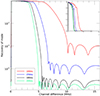 |
Fig. 1. Recovery of signal power in a given spectral differencing mode after application of a foreground filter to the full-band data (30.72 MHz). Inset shows the same data with a linear scaling. A 180 ns delay filter provides sufficient recovery on scales of interest (Δν < 4 MHz), but with a small correction required. |
We start by demonstrating the effect of the filter on the output of the MAPS algorithm. The ergodic MAPS algorithm is considered, most akin to the power spectrum, whereby only the spectral difference is considered, and the data are aggregated.
3.2. MAPS – no filter
Figure 2 (dashed) shows the output of MAPS for the same 192 channels (15 MHz) at the lower end of the high-band data (z = 6.8 − 7.5), but without the 180 ns filter, for eight computed l modes. Note that l = 100 corresponds to k⊥ = l/DM = 0.017 h Mpc−1. The power is consistently high across all estimated l-modes, with performance worsening on scales larger than 3 MHz. These values exceed the expected 21 power by at least six orders of magnitude, and are not useable for science.
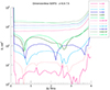 |
Fig. 2. Comparison of MAPS outputs without (dashed) and with (solid) the 180 ns filter for 192 channels in z = 6.8 − 7.5 for eight measured l-bins, where ‘NF’ denotes no filter being applied. |
3.3. Filtered MAPS – ergodic
The output of Eq. (10) is plotted for the first eight l modes for the same z = 6.8 − 7.5 set with the 180 ns filter, using logarithmic scales (Fig. 2, solid lines). The absolute value is plotted, but, in general, some modes are negative owing to the filter response. A correction is applied to the power for spectral differences smaller than 4 MHz to alleviate the small signal loss that occurs due to the filter. It is clear that application of the filter reduces the signal by approximately 2−5 orders of magnitude depending on scale, and therefore is worthwhile to apply. There are noticeable features present in the filtered MAPS, however, and these correspond to the oscillatory structure observed in the filter response in Fig. 1. Further tuning of the filter may be of benefit, but for these data is unlikely to yield further improvements.
Excellent results are produced for l = 100, 200, with larger modes showing commensurately poorer results in line with the l2 scaling of the dimensionless MAPS. As a comparison, the 21cmFAST cube output is shown for the same redshift range, and binning (Fig. 3). The results are similar to those in Mondal et al. (2022), but with lower amplitude, commensurate with the higher redshift of this cube. In general, the data yield MAPS amplitudes two orders of magnitude higher than the simulated signal, matching the Fourier power spectrum results produced for the Trott et al. (2020) work.
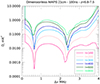 |
Fig. 3. Comparison of 21cmFAST simulated MAPS for z = 6.8 − 7.5. |
We also plot the first three l-modes for the full data (no filter), full data (180 ns filter), the 21 cm simulation (with filter), and the data noise level, in Fig. 4. The filter is again shown to have an impact on the contaminating power, but the data remain above the expected noise level, and the 21 cm signal power. The measured power bias relative to the thermal noise is evidence of residual systematics in the data. These plots also demonstrate that these data are not sufficient to detect this model signal, even in the absence of systematics, but are within an order of magnitude.
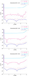 |
Fig. 4. Dimensionless MAPS for z = 6.8 − 7.5 for 192 80 kHz channels and the first three l-modes, showing the full data (no filter), full data (180 ns filter), the 21 cm simulation (with filter), and the data noise level. |
3.4. Filtered MAPS – local
The local MAPS treats the power for each set of two spectral channels individually, without averaging. Without the assumption of ergodicity, it can be applied to the full-band (30.72 MHz) data as long as we only consider spectral differences for which the filter does not suppress signal (Δν < 4 MHz).
Figure 5 shows contour plots of the dimensionless MAPS as a function of frequency, for l = 200, 300. The inset shows a subset of the data for clarity. The data have been corrected for the signal loss due to the 180 ns filter for Δν < 4 MHz. The red diagonal stripe at a spectral difference of ∼4 MHz is an artifact of the filter (where the cross power is transitioning from positive to negative, and the ratio of the power to the weights is undefined). Spectral separations larger than 4 MHz have been omitted. In general, there are frequencies (redshifts) where the MAPS is enhanced. Figure 6 then shows the equivalent filtered MAPS for the 21 cm simulation. The same filter artifact can be observed here.
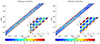 |
Fig. 5. Contour maps of dimensionless MAPS for the data and l = 200, 300. Note the different colour scale for each plot. |
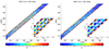 |
Fig. 6. Contour maps of dimensionless MAPS for the 21 cm simulation and l = 200, 300. Note the different colour scale for each plot. |
Figure 7 then shows the contrast ratio between the expected 21 cm power and the measured data (logarithmic scale). The scale is kept the same for both l-modes to show the differences. Greatest contrast is seen for l = 200 (k⊥ = 0.034 h Mpc −1) where the contrast ratio is generally 102 − 103, but observed as low as 101 in some regions. The contrast is poorer than for the ergodic MAPS, where data averaging reduces the noise and systematics further. We also tried averaging the data to 160 kHz resolution, and performing the local MAPS on those data. As expected, the contrast between 21 cm signal and the data did not change significantly, due to the data being systematics-limited.
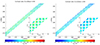 |
Fig. 7. Contour maps of contrast ratio of the 21 cm power to the data, for l = 200, 300. The logarithm is plotted, showing a 102 − 103 ratio of data to the expected signal power. |
4. Angular power spectrum
The data were also used to compute the single frequency angular power spectrum, to connect with more traditional studies of this statistic, and corresponding to the ν1 = ν2 term of Eqs. (4) and (9). All spectral channels are foreground dominated, and so the same filter was applied to reduce the level of contamination. The single channel case also allows for the data distribution to be studied, in contrast to the sample variance estimator, which uses all of the data blindly in the summation described in Eq. (9).
Figure 8 shows data, 21 cm and noise dimensionless angular power spectra as a function of l and for a set of redshifts, after application of the same 180 ns filter. The data are binned into coarse Δl = 100 (Δk⊥ = 0.016 h Mpc−1) bins, and have been averaged over the central 880 kHz in each 1.28 MHz coarse channel. The filtered data show the lowest values at low redshift, but are significantly higher than the expected signal with a contrast that exceeds that observed in the spherically averaged power spectrum, but only by a factor of 3−5. The expected 21 cm signal is also lowest at this redshift. The residual foreground power in each spectral channel is therefore less easily treated with the filter than with a line-of-sight spectral transform, but the results are not too degraded compared with the spherically averaged power spectrum, and allow for greater granularity to study the signal evolution.
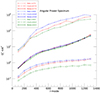 |
Fig. 8. Angular power spectra, |

The variance (power spectrum) can also be extracted from the data histograms. Typically, the data would be expected to be close to Gaussian-distributed, reflecting the near-Gaussian expectation for the signal, and the Gaussian radiometric noise. Estimation of the data variance directly from the sample data histograms should yield the same value as the sample variance computation (which is used for power spectrum estimation normally, e.g. Eq. (9)). Presence of bright foregrounds may skew this distribution, leading to outlier k-modes in the dataset.
To compute the sample data distributions, the real and imaginary components of the gridded visibilities were used to compute a histogram of the data for each l-mode, and at each coarse channel, with data being combined across spectral channels to form an effective 880 kHz bandwidth. A Gaussian was then fitted to the gridded visibilities of the ‘totals’ and the ‘differences’ to estimate the sample variance. A histogram resolution of 0.1 mK was chosen to avoid discretization effects. Figure 9 (left) shows example histogrammed data for the dimensionless angular power spectrum for totals visibilities (red) and the differenced visibilities (blue), for l = 200 and z = 6.8. Figure 9 (right) shows the comparison of the angular power spectra using the sample variance (dashed) and computed from Gaussian fits to the histograms (solid). Use of the histograms generally yielded improved results (lower power) across redshift and angular mode. At l = 200, where some of the best results have been found with these data, the angular power is 53 mK2 at z = 7.5, compared with the 21 cm simulated power of 0.05 mK2, yielding a data-to-signal contrast ratio of ∼1000, which exceeds that found in Trott et al. (2020) for the spherically averaged power spectrum with the same data, by a factor of 3−5. A similar ratio is obtained at l = 100, where the measured power is Δ2 = 10 mK2.
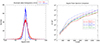 |
Fig. 9. Angular power spectrum extraction. Left: histograms of the real and imaginary components of the gridded visibilities for a 880 kHz band at z = 6.8 and l = 200. Right: angular power spectra across three redshifts using the normal sample variance estimate (dashed) and extracted from fits to the histograms (solid). |
5. Discussion
The foreground filter does a reasonable job of removing a lot of the correlated spectral structure, but there remains spectral structure on EoR scales that leaves excess power in the MAPS. In spherically averaged power spectrum estimation, a line-of-sight spectral transform must be performed to move from configuration to k-space, and this is problematic due to the data being discrete and band-limited. Typically, a spectral taper is applied prior to transform to suppress sidelobes, but this is prone to error when applied to discrete data, and comes at the expense of a broader main lobe (correlating line-of-sight k-modes). Several groups have studied the effect of the taper application and spectral transform on leakage of foreground power into EoR modes (e.g., Lanman et al. 2020; Barry & Chokshi 2022), showing that leaked power can be a source of excess power. With MAPS, no such transform is required, and foregrounds need to be treated separately. Thus, the residual (excess) power relative to the noise level observed in these data is indicative of inherent spectral variability on those scales, and not from leaked power from larger modes. This conclusion is not unreasonable, because the data calibration only considered unpolarized point sources and extended foregrounds, with unpolarized diffuse and polarized diffuse, and point source models omitted. Polarized emission, which is known to be significant in this observing field (Bernardi et al. 2013; Lenc et al. 2017) will imprint spectral structure for sources with non-zero Faraday depth. In general, the single-frequency angular power spectrum yields a higher contrast ratio than the local MAPS, suggesting that there are benefits to considering small spectral differences, where the 21 cm signal power is reduced, but the foregrounds also partially decohere.
6. Conclusions
The Multi-Frequency Angular Power Spectrum (MAPS) has been applied to a deep 110-h integration of the EoR0 field from the MWA EoR project in z = 6.5 − 7.5. These data have been previously used with a spherically averaged power spectrum to produce scientifically relevant upper limits on the power spectrum of brightness temperature fluctuations in the hyperfine transition line of cosmological neutral hydrogen. The angular power spectrum has the advantage of not requiring a band-limited line-of-sight spectral transform, which mixes line-of-sight k-modes and needs to be performed on (approximately) ergodic subsets of a full dataset. However, it suffers from contamination from residual continuum foreground signal, which is highly dominant and cannot easily be distinguished without spectral information. Here, a filter is applied to the broadband dataset prior to estimation of the angular power spectrum, to remove smoothly varying signal structure. This improves the power spectrum estimation by two orders-of-magnitude, but still yields poorer results relative to the expected 21 cm signal compared with the spherically averaged power spectrum.
Treatment of foregrounds differs between the angular and spherically averaged power spectrum approaches; the former using a filter with the latter using the properties of the Fourier Transform. The filter employed here is shown to improve its performance with larger initial bandwidths (Ewall-Wice et al. 2021), whereas the Fourier Transform cannot be used over bandwidths that destroy the assumption of signal ergodicity. Thus, increasing the bandwidth of experimental data may improve the performance of the APS compared with the spherically averaged power spectrum. Additionally, other foreground filters may be explored and employed (Pal et al. 2021). In future, a combination of spectral and spatial (e.g., GMCA, Chapman et al. 2014) filtering may be required to yield improved results.
In an optimal power spectrum estimator, the gridding kernel is the Fourier Transform of the telescope response function to the sky (i.e., the beam), because this correctly represents the smearing of information due to the finite station size. In practise, the MWA beam is highly structured with sidelobes, and we instead employ a size-matched Blackman Harris 2D window function as the kernel, as is done in Trott et al. (2016).
Acknowledgments
This research was partly supported by the Australian Research Council Centre of Excellence for All Sky Astrophysics in 3 Dimensions (ASTRO 3D), through project number CE170100013. C.M.T. is supported by an ARC Future Fellowship under grant FT180100321. The International Centre for Radio Astronomy Research (ICRAR) is a Joint Venture of Curtin University and The University of Western Australia, funded by the Western Australian State government. The MWA Phase II upgrade project was supported by Australian Research Council LIEF grant LE160100031 and the Dunlap Institute for Astronomy and Astrophysics at the University of Toronto. This scientific work makes use of the Murchison Radio-astronomy Observatory, operated by CSIRO. We acknowledge the Wajarri Yamatji people as the traditional owners of the Observatory site. Support for the operation of the MWA is provided by the Australian Government (NCRIS), under a contract to Curtin University administered by Astronomy Australia Limited. We acknowledge the Pawsey Supercomputing Centre which is supported by the Western Australian and Australian Governments. Data were processed at the Pawsey Supercomputing Centre. R.M. is supported by the Wenner-Gren Postdoctoral Fellowship and GM acknowledges support by Swedish Research Council grant 2020-04691. R.M. is also supported by the Israel Academy of Sciences and Humanities & Council for Higher Education Excellence Fellowship Program for International Postdoctoral Researchers.
References
- Barry, N., & Chokshi, A. 2022, ApJ, 929, 64 [NASA ADS] [CrossRef] [Google Scholar]
- Barry, N., Beardsley, A. P., Byrne, R., et al. 2019, PASA, 36, e026 [NASA ADS] [CrossRef] [Google Scholar]
- Bernardi, G., Greenhill, L. J., Mitchell, D. A., et al. 2013, ApJ, 771, 105 [Google Scholar]
- Bharadwaj, S., & Ali, S. S. 2005, MNRAS, 356, 1519 [NASA ADS] [CrossRef] [Google Scholar]
- Bowman, J. D., Cairns, I., Kaplan, D. L., et al. 2013, PASA, 30, 31 [NASA ADS] [CrossRef] [Google Scholar]
- Bowman, J. D., Rogers, A. E. E., Monsalve, R. A., Mozdzen, T. J., & Mahesh, N. 2018, Nature, 555, 67 [Google Scholar]
- Chapman, E., Zaroubi, S., & Abdalla, F. 2014, MNRAS, 458, 2928 [Google Scholar]
- Datta, K. K., Choudhury, T. R., & Bharadwaj, S. 2007, MNRAS, 378, 119 [CrossRef] [Google Scholar]
- DeBoer, D. R., Parsons, A. R., Aguirre, J. E., et al. 2017, PASP, 129, 045001 [NASA ADS] [CrossRef] [Google Scholar]
- Ewall-Wice, A., Kern, N., Dillon, J. S., et al. 2021, MNRAS, 500, 5195 [Google Scholar]
- Greig, B., Wyithe, J., Murray, S. G., Mutch, S. J., & Trott, C. M. 2022, MNRAS, 516, 5588 [NASA ADS] [CrossRef] [Google Scholar]
- Koopmans, L., Pritchard, J., Mellema, G., et al. 2015, Proceedings of Advancing Astrophysics with the Square Kilometre Array (AASKA14). 9 -13 June, 2014. Giardini Naxos, Italy. Online at http://pos.sissa.it/cgi-bin/reader/conf.cgi?confid=215, 1 [Google Scholar]
- Lanman, A. E., Pober, J. C., Kern, N. S., et al. 2020, MNRAS, 494, 3712 [NASA ADS] [CrossRef] [Google Scholar]
- Lenc, E., Anderson, C. S., Barry, N., et al. 2017, PASA, 34, e040 [Google Scholar]
- Line, J. L. B. 2022, J. Open Sour. Softw., 7, 3676 [NASA ADS] [CrossRef] [Google Scholar]
- Mesinger, A., Furlanetto, S., & Cen, R. 2011, MNRAS, 411, 955 [Google Scholar]
- Mondal, R., Bharadwaj, S., & Datta, K. K. 2018, MNRAS, 474, 1390 [NASA ADS] [CrossRef] [Google Scholar]
- Mondal, R., Bharadwaj, S., Iliev, I. T., et al. 2019, MNRAS, 483, L109 [CrossRef] [Google Scholar]
- Mondal, R., Shaw, A. K., Iliev, I. T., et al. 2020, MNRAS, 494, 4043 [NASA ADS] [CrossRef] [Google Scholar]
- Mondal, R., Mellema, G., Murray, S. G., & Greig, B. 2022, MNRAS, 514, L31 [Google Scholar]
- Pal, S., Bharadwaj, S., Ghosh, A., & Choudhuri, S. 2021, MNRAS, 501, 3378 [NASA ADS] [Google Scholar]
- Park, J., Mesinger, A., Greig, B., & Gillet, N. 2019, MNRAS, 484, 933 [NASA ADS] [CrossRef] [Google Scholar]
- Parsons, A. R., & Backer, D. C. 2009, AJ, 138, 219 [NASA ADS] [CrossRef] [Google Scholar]
- Santos, M. G., Cooray, A., & Knox, L. 2005, ApJ, 625, 575 [NASA ADS] [CrossRef] [Google Scholar]
- Singh, S., Nambissan, J., Subrahmanyan, R., et al. 2022, Nat. Astron., 6, 607 [NASA ADS] [CrossRef] [Google Scholar]
- Thekkeppattu, J. N., McKinley, B., Trott, C. M., Jones, J., & Ung, D. C. X. 2022, PASA, 39, e018 [NASA ADS] [CrossRef] [Google Scholar]
- Tingay, S. J., Goeke, R., Bowman, J. D., et al. 2013, PASA, 30, 7 [Google Scholar]
- Trott, C. M., Pindor, B., Procopio, P., et al. 2016, ApJ, 818, 139 [NASA ADS] [CrossRef] [Google Scholar]
- Trott, C. M., Jordan, C. H., Midgley, S., et al. 2020, MNRAS, 493, 4711 [NASA ADS] [CrossRef] [Google Scholar]
- van Haarlem, M. P., Wise, M. W., Gunst, A. W., et al. 2013, A&A, 556, A2 [NASA ADS] [CrossRef] [EDP Sciences] [Google Scholar]
- Wayth, R. B., Tingay, S. J., Trott, C. M., et al. 2018, PASA, 35, E033 [NASA ADS] [CrossRef] [Google Scholar]
All Figures
|
Fig. 1. Recovery of signal power in a given spectral differencing mode after application of a foreground filter to the full-band data (30.72 MHz). Inset shows the same data with a linear scaling. A 180 ns delay filter provides sufficient recovery on scales of interest (Δν < 4 MHz), but with a small correction required. |
| In the text | |
|
Fig. 2. Comparison of MAPS outputs without (dashed) and with (solid) the 180 ns filter for 192 channels in z = 6.8 − 7.5 for eight measured l-bins, where ‘NF’ denotes no filter being applied. |
| In the text | |
|
Fig. 3. Comparison of 21cmFAST simulated MAPS for z = 6.8 − 7.5. |
| In the text | |
|
Fig. 4. Dimensionless MAPS for z = 6.8 − 7.5 for 192 80 kHz channels and the first three l-modes, showing the full data (no filter), full data (180 ns filter), the 21 cm simulation (with filter), and the data noise level. |
| In the text | |
|
Fig. 5. Contour maps of dimensionless MAPS for the data and l = 200, 300. Note the different colour scale for each plot. |
| In the text | |
|
Fig. 6. Contour maps of dimensionless MAPS for the 21 cm simulation and l = 200, 300. Note the different colour scale for each plot. |
| In the text | |
|
Fig. 7. Contour maps of contrast ratio of the 21 cm power to the data, for l = 200, 300. The logarithm is plotted, showing a 102 − 103 ratio of data to the expected signal power. |
| In the text | |
|
Fig. 8. Angular power spectra, |
| In the text | |
|
Fig. 9. Angular power spectrum extraction. Left: histograms of the real and imaginary components of the gridded visibilities for a 880 kHz band at z = 6.8 and l = 200. Right: angular power spectra across three redshifts using the normal sample variance estimate (dashed) and extracted from fits to the histograms (solid). |
| In the text | |
Current usage metrics show cumulative count of Article Views (full-text article views including HTML views, PDF and ePub downloads, according to the available data) and Abstracts Views on Vision4Press platform.
Data correspond to usage on the plateform after 2015. The current usage metrics is available 48-96 hours after online publication and is updated daily on week days.
Initial download of the metrics may take a while.