| Issue |
A&A
Volume 672, April 2023
|
|
|---|---|---|
| Article Number | A100 | |
| Number of page(s) | 12 | |
| Section | The Sun and the Heliosphere | |
| DOI | https://doi.org/10.1051/0004-6361/202243912 | |
| Published online | 05 April 2023 | |
Optimal stereoscopic angle for 3D reconstruction of synthetic small-scale coronal transients using the CORAR technique
1
Deep Space Exploration Laboratory/School of Earth and Space Sciences, University of Science and Technology of China, Hefei, Anhui 230026, PR China
e-mail: ymwang@ustc.edu.cn, lsy1997@mail.ustc.edu.cn
2
CAS Center for Excellence in Comparative Planetology/CAS Key Laboratory of Geospace Environment/Mengcheng National Geophysical Observatory, University of Science and Technology of China, Hefei, Anhui 230026, PR China
3
Collaborative Innovation Center of Astronautical Science and Technology, Hefei, Anhui 230026, PR China
Received:
30
April
2022
Accepted:
22
February
2023
Context. In previous studies, we applied the CORrelation-Aided Reconstruction (CORAR) technique to reconstruct three-dimensional (3D) structures of transients in the field of view (FOV) of Heliospheric Imager-1 (HI-1) on board the spacecraft STEREO-A/B. The reconstruction quality depends on the stereoscopic angle (θSun), that is, the angle between the lines connecting the Sun and two spacecraft.
Aims. To apply the CORAR technique on images from the coronagraphs COR-2 on board STEREO, the impact of θSun on the reconstruction of coronal transients should be explored, and the optimal θSun for reconstruction should be found.
Methods. We apply the CORAR method on synthetic COR-2 images containing the small-scale transient, namely the blob, in the case of various θSun. Based on a comparison of the synthetic blob and the corresponding reconstructed structure in location and 3D shape, we assess its level of reconstruction quality. According to the reconstruction-quality levels of blobs in various positions with various attributes, we evaluate the overall performance of reconstruction in the COR-2 FOV to determine the optimal θSun for reconstruction.
Results. In the case of θSun > 90°, we find that the range of suitable θSun, in which the small-scale transients in the COR-2 FOV typically have high reconstruction quality, is between 120° and 150°, and the optimal θSun for reconstruction is close to 135°. In the case of θSun < 90°, the global reconstruction performance is similar to that of (180° −θSun). We also discuss the spatial factors in determining the range of suitable θSun, and study the influence of blob properties on the reconstruction. Our work can serve as a foundation for the design of future missions containing coronagraphs from multiple perspectives, such as the newly proposed SOlar Ring mission (SOR).
Key words: Sun: corona / Sun: heliosphere / solar wind
© The Authors 2023
 Open Access article, published by EDP Sciences, under the terms of the Creative Commons Attribution License (https://creativecommons.org/licenses/by/4.0), which permits unrestricted use, distribution, and reproduction in any medium, provided the original work is properly cited.
This article is published in open access under the Subscribe to Open model. Subscribe to A&A to support open access publication.
1. Introduction
Many inhomogeneous structures of different spatial and temporal scales exist in the solar wind, originating from the Sun or forming en route as the solar wind propagates outward (Viall et al. 2021). A typical example of large-scale transients is the coronal mass ejection (CME), which injects significant amounts of plasma into the heliosphere and is capable of triggering dramatic changes in space weather if arriving at the Earth (Gosling et al. 1990; Manoharan 2006; Balan et al. 2014). On the other hand, there are also many small-scale transients in the interplanetary space, such as switchbacks and blobs. Defined as S-shaped magnetic structures, switchbacks are discovered frequently by the Parker Solar Probe (PSP, Fox et al. 2016) in the inner heliosphere (Kasper et al. 2019; Horbury et al. 2020) and may be observed by coronagraphs (Telloni et al. 2022). Blobs are small and discrete transients propagating radially from the boundaries of coronal holes or the top of coronal streamers, and generally have initial sizes of about 0.1−1 solar radii (R⊙) at 3 − 4 R⊙ from the Sun (Sheeley et al. 1997; Wang et al. 1998; López-Portela et al. 2018). Blobs are released periodically because of the intermittent reconnection of magnetic field, and they are regarded as important parts of slow solar wind in observations (Sheeley et al. 2009; Sheeley & Rouillard 2010; Viall & Vourlidas 2015; Sanchez-Diaz et al. 2017a,b). The properties and evolution of solar-wind transients arising from or near the Sun contain imprints of the environment below the corona (Hundhausen et al. 1968; Ko et al. 1997; Landi et al. 2012), which may help us understand the nature of the solar atmosphere.
The most direct method to identify the transients near the Sun is through remote imaging. White-light imagers observing the solar corona and the heliosphere in the visible-light wavelength are widely used because of their sensitivity to the variation of the electron density and location of transients according to Thomson scattering theory (Vourlidas & Howard 2006; Howard & DeForest 2012; DeForest et al. 2013a; Howard et al. 2013; Inhester 2015). Many spacecraft are loaded with coronagraphs or heliospheric imagers. The Large Angle and Spectrometric Coronagraph (Brueckner et al. 1995) on board the Solar and Heliospheric Observatory (Domingo et al. 1995) has been observing the outer corona and heliosphere since 1996. Simultaneous observations from two different viewpoints are provided by the coronagraphs (COR-1 and COR-2) and heliospheric imagers (HI-1 and HI-2, Harrison et al. 2005) in the SECCHI suite (Howard et al. 2008) on board the Solar Terrestrial Relations Observatory (STEREO, Kaiser et al. 2008). Launched in recent years, the Parker Solar Probe (Fox et al. 2016) can observe fine structures of CMEs at a closer distance from the Sun with its Wide-field Imager for Solar PRobe (WISPR, Vourlidas et al. 2016). Solar Orbiter (Müller 2020) can provide observations from a high-latitude viewpoint by the imager SoloHi (Howard et al. 2020) and coronagraph Metis. Different techniques have been developed to derive three-dimensional (3D) information about the locations and velocities of transients from white-light images. The forward-modeling techniques were developed to obtain the kinematic parameters of CMEs by fitting geometrical models, such as ice-cream cone or GCS model (Zhao et al. 2002; Xie et al. 2004; Xue et al. 2005; Thernisien et al. 2006, 2009; Zhao 2008; Thernisien 2011). The direction and velocity of propagating transients can be estimated using the trace-fitting methods, such as Point-P, Fixed-ϕ, Harmonic Mean, and Self-Similar Expansion (Sheeley et al. 1999; Howard et al. 2006; Davies et al. 2012, 2013; Moestl & Davies 2013; Wang et al. 2013; Volpes & Bothmer 2015). Using the polarization ratio technique (Moran & Davila 2004; Dere et al. 2005; Moran et al. 2010; Susino et al. 2014; DeForest et al. 2017; Bemporad et al. 2018), the density-weighted center of transients can be located along the line of sight. Based on multi-view observations, methods such as Tie-pointing, Geometric Localization, Mask Fitting and Local Correlation Tracking (Pizzo & Biesecker 2004; Inhester 2006; Mierla et al. 2008, 2009, 2010; de Koning et al. 2009; Feng et al. 2012, 2013) can be used to measure the locations of transients by triangulation.
Based on triangulation, Li et al. (2018, 2020) developed the CORrelation-Aided Reconstruction (CORAR) method to locate and reconstruct solar wind transients in the 3D space using a correlation analysis of STEREO/HI-1 images from two perspectives. This method was further developed to generate the radial velocity map of transients with the maximum correlation-coefficient localization and cross-correlation tracking (MCT) method (Li et al. 2021). The stereoscopic angle (θSun), that is, the angle between the lines connecting the Sun and two spacecraft, has a significant influence on the accuracy of triangulation methods. For instance, the geometric localization method provides the most precise results when θSun is between 30° and 150° (de Koning et al. 2009). As to the Tie-pointing technique, the reconstruction error of transients from the positional uncertainty along the epipolar lines on images is dependent on θSun (Inhester 2006; Wiegelmann et al. 2009; Mierla et al. 2010). Inhester (2006) discussed the identification of loops in the case of θSun < 90°, in which features on different images are more similar with smaller θSun. Mierla et al. (2010) grouped the errors of reconstruction into observational and methodical errors, and pointed out that θSun close to 90° will be beneficial for a strict stereo reconstruction but will lead to more serious misidentification of similar features on images at the same time. Lugaz (2010) find some evidence that direct triangulation in the HI fields of view (FOVs) should only be applied to CMEs propagating approximatively toward Earth, that is, within 20° from the Sun–Earth line. When the range of spacecraft separation is less than 50°, the Tie-pointing and Triangulation method gives reliable trajectories for CMEs propagating within about 40° elongation from the plane of sky (Liewer et al. 2011). For the CORAR technique, we prove that structures of reconstructed transients in the HI-1 FOV are credible when the θSun is about 120° −150° (Lyu et al. 2020, 2021). For large-scale transients like CMEs, the optimal θSun for reconstruction tends to 150°, and so their structures can be reconstructed more completely; for small-scale transients, such as blobs, optimal θSun for reconstruction tends to 120° because the uncertainties of triangulation are reduced at this angle. When θSun is closer to 180° and transients are closer to the connecting line of two spacecraft, the triangulation of transients is less accurate and the reconstructed structures may bloat in the direction of the connecting line of two spacecraft, which is called the collinear effect (Li et al. 2018).
To further investigate the evolution of transients in the outer corona, we would also like to apply the CORAR method to the images observed by COR-2 on board STEREO. Because COR-2 observes transients closer to the Sun, the performance of reconstruction of transients observed by COR-2 should be different from those observed by HI-1 in terms of brightness and geometry, and the optimal θSun for reconstruction in the HI-1 FOV may be unsuitable in the COR-2 FOV. Therefore, the reconstruction performance of the CORAR technique based on COR-2 images must be investigated. Our study may also provide the basis for other orbital schemes containing multiple satellites, such as the SOlar Ring mission (SOR, Wang et al. 2020, 2021), the aim of which is to simultaneously observe the 360° surface of the Sun and the inner heliosphere. In the current SOR scheme, three spacecraft loaded with wide-FOV coronagraphs are separated by 120° in a circumsolar orbit, with one spacecraft separated from the Earth by 30° (Wang et al. 2023). In Sect. 2, we introduce a test of the reconstruction performance for different θSun using synthetic COR-2 images of blobs. We also introduce the improved CORAR technique for COR-2 images and a definition of the classification of reconstruction quality. The results of cases with different θSun are presented in Sect. 3 to derive the optimal θSun in the COR-2 FOV. The factors influencing the range of suitable θSun for reconstruction are discussed in Sect. 4, and a summary is given in Sect. 5. Two Appendices provide additional information and figures that support our study and give a detailed explanation of the improved CORAR method.
2. Method
2.1. Reconstruction of a blob on synthetic COR-2 images
The STEREO twin spacecraft Ahead and Behind were launched in 2006. They orbit the Sun at approximately 1 AU near the ecliptic plane with a slowly increasing angle of about 45° per year between them. The θSun increased from 90° to 150° during the time from May 2009 to August 2010. The coronagraphs COR-2 on board STEREO can observe the outer corona in the range from 2.5 to 15 solar radii from the Sun in the plane of sky (POS).
In our study, a synthetic blob made by a ball model (Li et al. 2020; Lyu et al. 2020) is inserted into the 3D space in the COR-2 FOV so that it can be observed from COR-2A and COR-2B perspectives. We generate the synthetic COR-2 images containing the blob for reconstruction, and study the reconstructed structure of the blob with specific location and properties in the case of selected θSun. The 3D reconstruction is implemented in the Heliocentric Earth Ecliptic (HEE) coordinate system (Thompson 2006). For instance, Fig. 1a displays the FOV of two STEREO spacecraft observing the blob located at 0° in latitude, 30° in longitude, and 10⊙ in heliocentric distance when θSun is 135°. Figures 1b–d present the 3D structure of the synthetic blob and the synthetic images observed from COR-2A and COR-2B perspectives. The images only contain the blob without other coronal transients and streamers. In real observations, transients far away from the Sun are more distinguishable on COR-2 images processed by the normalizing-radial-gradient filter (NRGF; Morgan et al. 2006). This filter first subtracts the average brightness of each height from the images, and then divides images by the standard deviation of values at the same height. We therefore use synthetic NRGF-processed images as input for the CORAR technique to output the 3D structure of the blob.
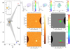 |
Fig. 1. CORAR reconstruction of a synthetic blob. The location of the blob in the HEE coordinate is 0° in latitude, 30° in longitude, and 10 R⊙ in heliocentric distance. The number density at the center of the blob is about 3.5 × 104 cm−3. The separation angle between the Earth and the spacecraft STEREO-A/B is about 65°/71°. Panel a: coordinates of STEREO-A (STA), STEREO-B (STB), the Sun, and the synthetic blob. The STA-Sun-STB angle (θSun) and the STA-blob-STB angle (θblob, namely the opening angle in the text) are highlighted. LAB is defined as the connecting line of two spacecraft. Panel b: 3D presentation of the synthetic blob. Panels c and d: synthetic COR-2A and COR-2B images containing the blob. Panel e: 3D presentation of cc that represents the reconstructed structure (see the context in Sect. 2). Panel f: reconstructed structure in the X − Y plane. The half thickness rAB of the reconstructed structure in the direction of LAB is labeled. Panels g and h: reconstructed structure observed from the COR-2A and COR-2B perspectives. The maximum radii of the reconstructed blob on COR-2A and COR-2B images, i.e., maximum rA and rB, respectively, are labeled. |
Based on triangulation, the method CORAR is used for the detection, localization, and 3D reconstruction of solar-wind inhomogeneous transients observed from dual perspectives of STEREO-A and -B. There are three main steps to the CORAR method: (1) Choose a meridian plane, that is, a plane containing the z-axis in the HEE coordinate, and project the images from two spacecraft onto the meridian plane along the line of sight (LOS). (2) Calculate the Pearson correlation coefficient (cc) of two projected images with suitable sampling boxes; the cc will have a high value in the position where transients exist. (3) Choose other meridian planes with different longitude, and then repeat the steps above to obtain the distribution of the cc in the 3D space. According to the 3D cc map, we recognize the high-cc regions, defined by cc > 0.5, as the reconstructed structures of solar-wind transients in 3D space. In Li et al. (2020) and Lyu et al. (2020), we found a discrepancy between the reconstructed structure and the precise structure of the synthetic blob in the HI-1 FOV. The morphological error is related to the position and properties of transients, the θSun, the image quality, and so on. Therefore, the high-cc regions are not the precise 3D structures of transients, but we can locate the real transients and obtain an estimation of their 3D shapes from the high-cc regions, as shown by the comparison of the synthetic blob and its reconstructed structure in Figs. 1b and e. The sampling boxes of step (2) have different lengths in the dimensions of time, heliocentric distance, and latitude. The temporal length of the sampling box is set as three frames to reduce false high-cc structures. To better reconstruct coronal transients with variant scales, the CORAR technique is improved so that the size of sampling boxes in heliocentric distance and latitude is adjusted automatically according to the sizes of the transients (see Appendix A).
2.2. Assessment of the reconstruction quality of a blob
The reconstruction quality of a synthetic blob is evaluated based on the following three conditions:
-
Recognition (R): We test whether the reconstructed blob can be detected at its 3D position. A blob can be recognized by the CORAR technique if there are high-cc regions (cc > 0.5) in the 3D space containing the initial synthetic blob.
-
Location (L): We test the accuracy with which the 3D structure of the reconstructed blob is located. The deviation of the position of the reconstructed structure from the position of its corresponding synthetic blob (Δl) is calculated by Eq. (1), and (x0, y0, z0) is the center of the synthetic blob. The blob is accurately located if Δl is less than 0.1 blob radii (rblob).
-
Shape (S): We compare the reconstructed structure with its corresponding synthetic blob in terms of shape. We measure the range of the radius of reconstructed blobs in the FOV of COR-2A and COR-2B, respectively (rA and rB, see Figs. 1g and h), and in the direction of the connecting line of two spacecraft (LAB) we measure the half thickness of reconstructed structures (rAB, see Fig. 1f). The blob is reconstructed with high creditability if rA, rB, and rAB are always within 0.6−1.4 rblob .
With the rules defined above, we examine whether a blob can be detected and accurately located, and to what extent its shape can be reconstructed in accordance with the images. In particular, we investigate the thickness of the reconstructed blob in the direction of LAB, and regard it as an estimator of the collinear effect and the completeness of the reconstructed structure: with rAB smaller than 0.6 rblob, the reconstructed blob is incomplete; with rAB larger than 1.4 rblob, the reconstructed blob may bloat seriously. The ranges of the parameters for condition R, L, and S are determined empirically to divide the reconstruction quality into four levels (Table 1): Level 0, the blob is not detected; Level 1, the blob is detected and reconstructed (R); Level 2, the blob is reconstructed and accurately located (R+L); Level 3, the blob is reconstructed, is located, and has the same shape as the synthetic blob (R+L+S). Level 3 is the highest level of reconstruction performance and Level 0 is the lowest. Therefore, we can assess the reconstruction quality of a blob with specific location and properties in the case of selected θSun.
Levels of 3D reconstruction quality of the synthetic blob.
2.3. The global reconstruction quality of blobs in the COR-2 FOV
In the previous sections, we introduce the reconstruction and assessment of one blob. Next, we modify the position of the blob, and repeat the process described in the previous sections for blobs in different locations. Therefore, we can study the 3D distribution of different levels of reconstruction quality of blobs in SCOR2, that is, the 3D space in the COR-2 FOV (see Fig. 2a). The locations of the blob are arranged in a 3D grid in the HEE coordinate, with a grid spacing of 1 R⊙ in the radial direction, and 10° in both latitudinal and longitudinal directions. We select positions in half of the angular space to be tested due to the 180° periodicity of the reconstruction quality of transients in longitude (see more details in Appendix B).
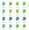 |
Fig. 2. Three-dimensional distributions of blobs at different levels of reconstruction quality in Group 1 (panels a–d), Group 2 (panels e–h), Group 3 (panels i–l), and Group 4 (panels m–p) when θSun is 90° (panels a, e, i, and m), 120° (panels b, f, j, and n), 135° (panels c, g, k, and o), and 150° (panels d, h, l, and p). See the descriptions of different groups in the text and Table 2. |
Furthermore, we assess the global reconstruction quality of blobs in all positions. We measure the weighted reconstruction quality (WRQ), which is calculated using the following equation:
where NLi is the number of blobs at Level i of reconstruction quality. We select the coefficients aLi so that the global reconstruction quality is better when WRQ is closer to 1.
Parameters used in generating synthetic blobs.
2.4. Reconstruction of blobs under different conditions
Besides the location, the reconstruction performance of a synthetic blob also relies on its properties, including size, density, velocity, and so on. Real transients may expand during outward propagation, and so their properties vary with distance from the Sun. Therefore, we study the reconstruction of the blob under different conditions. We study two conditions that govern the state of a blob: 1. The self-similar expansion (SSE) condition: the blob self-similarly expands, and its size and density vary with its position, as in real propagating transients. Considering the possible pile-up of mass of transients from the background environment (Colaninno & Vourlidas 2009; DeForest et al. 2013b; Feng et al. 2015) or the constraint of internal magnetic field and ambient pressure (DeForest et al. 2018), we empirically select −2.4 as the attenuation index of density. 2. The nonSSE condition: the radius and the number density of a blob remain unchanged as its position changes. Under the SSE and nonSSE conditions, blobs with low and high number density are studied. Therefore, four groups of blobs are reconstructed to study the global reconstruction quality under different conditions: blobs of Groups 1 and 2 are under the nonSSE condition with low and high density, respectively, and blobs of Groups 3 and 4 are under the SSE condition with low and high density, respectively. Table 2 shows the parameters of synthetic blobs belonging to these four groups.
2.5. The selection of specific θSun
Finally, we compare the global reconstruction quality of the blobs of the four groups described above in the case of different θSun in order to study the influence of the variation of θSun on the reconstruction by the CORAR technique. As the cases of θSun may be similar to the cases of 180° −θSun (see Appendix B), we focus on cases with θSun of between 90° and 180°. Considering the optimal θSun for the HI-1 FOV (Lyu et al. 2020, 2021) and the orbital scheme of the Solar Ring mission, we study the global reconstruction quality of blobs when θSun is 90°, 120°, 135°, and 150° in order to derive the optimal θSun for the reconstruction of transients in the COR-2 FOV.
3. Optimal separation angle for COR-2 FOV
Figures 2a–h show the 3D distributions of levels of reconstruction quality of blobs under the nonSSE condition. Figures 3a and b display the WRQ and relative frequency of four reconstruction-quality levels at different θSun for non-SSE blobs with low and high density (Groups 1 and 2). When θSun is 135°, most blobs have the best reconstruction performance, and WRQ peaks in both cases of Group 1 and 2. A few blobs with low levels of reconstruction quality are located away from the meridian plane bisecting θSun in the 3D space, and are located close to the inner edge on COR-2 images. We obtain similar results for other cases with different θSun. In the case with θSun of 120°, WRQ is higher (lower) than that in the case with θSun of 150° when the number density is high (low). The difference is related to the frequency of Level-3 blobs. The reconstructed structures of blobs – with low density when θSun = 120° or with high density when θSun = 150° – have more difficulty in satisfying the condition S (see definition in Sect. 2.2), indicating that transients with higher density may require a smaller θSun for reconstruction. By comparing the frequency of blobs at Level 2 and Level 3, we find that blobs are more likely to be well located in the case with θSun of 150° than when θSun is 120°. As to 90°, most blobs with either low or high density are at Level 2 and unable to meet the condition S, and so the global reconstruction quality of these cases is poorer than the cases of 120° and 150°.
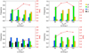 |
Fig. 3. Relative frequency of blobs of different levels of reconstruction quality and their WRQ (red lines) with different θSun. The blobs are of Group 1 (panel a), Group 2 (panel b), Group 3 (panel c), and Group 4 (panel d). The colors representing different levels of reconstruction quality are the same as those in Fig. 2. |
Under the SSE condition (Figs. 2i–p), the number of high-quality reconstructed blobs is significantly reduced compared to the non-SSE cases. Blobs located near the central meridian plane and at smaller distance from the Sun are more likely to have good reconstruction quality, especially in the case of low density (Figs. 2i–l). The trend of WRQ of SSE blobs is similar to that of nonSSE blobs, but the values of WRQ are clearly smaller due to high frequencies of Level-1 and Level-2 blobs (Figs. 3c and d). Under the SSE condition, blobs located further away from the Sun have lower signal-to-noise ratio (S/N) and larger scales on images. It is more difficult for the reconstructed blobs to satisfy the conditions L and S, which results in the high frequency of low-quality blobs in Figs. 3c and d.
Taking the four cases of different conditions into comprehensive consideration, the rank of overall reconstruction performance is 135° > 150° ≥120° > 90°. Therefore, the optimal θSun for the 3D reconstruction of transients in the COR-2 FOV is close to 135°, and the small-scale blob generally has good reconstruction quality when θSun is between 120° and 150°. Considering the geometrical symmetry, it is also suitable for reconstruction if θSun is close to 45° (see Appendix B). To study whether the result is influenced by the change in the conditions for assessing reconstruction quality, we analyze cases with different ranges of rA, rB, and rAB in the condition S, and find that the optimal θSun is identical.
4. Discussion
In Fig. 3, the optimal θSun for the four groups of blobs is comparable, while the range of θSun with high WRQ is different. Therefore, we explore the possible reasons why the optimal θSun is close to 135°, and discuss the factors that influence the global reconstruction quality of blobs.
4.1. Signal-to-noise ratio of the images
According to the Thomson Scattering theory, the brightness of coronal while-light images depends on the position and mass of transients under the condition of optically thin plasma (Howard & DeForest 2012; DeForest et al. 2013a; Howard et al. 2013). The S/N of the blob on images can be influenced by its location and density in the 3D space, as well as the image noise caused by stray light, star field, systematic problems, and so on. With higher S/N, the blob is more distinguishable from the background, and its successful reconstruction with the CORAR technique is more straightforward. Therefore, we are interested in the SS/N, that is, the 3D space where blobs could have good S/N on both COR-2A and COR-2B images for reconstruction, and its dependence on θSun.
We calculate the S/N of blobs on images from COR-2A and COR-2B perspectives (S/Na and S/Nb), and evaluate the total signal-to-noise ratio (TS/N) and the contrast between S/Na, b (DS/N) using the following equations (see Appendix B in Li et al. 2020)
where Ia, b and Ia, b0 represent the pixels from the image containing the synthetic blob and the background image without the blob, respectively, and N is the number of pixels for calculating the S/N. Blobs with low TS/N are indistinct on images, and blobs with high DS/N have a large difference in S/N between COR-2A and COR-2B images. Figure 4 shows the distribution of WRQ versus DS/N and TS/N for the blobs under the nonSSE and SSE conditions. Reconstructed transients with low DS/N and high TS/N are more likely to have good reconstruction quality. In many cases, TS/N can have any value and the reconstruction quality is still good for low DS/N. Figure 5 displays the distribution of Δl, rAB, maximum, and minimum rA versus TS/N and DS/N. This proves that reconstructed blobs with low DS/N and high TS/N are more likely to meet the condition L and S. According to the relationship between WRQ and S/N shown in Fig. 4, blobs with relatively good reconstruction performance possibly satisfy the following empirical S/N condition:
 |
Fig. 4. Two-dimensional distribution of the WRQ of the nonSSE (panels a–d) and SSE (panels e–h) blobs as a function of TS/N and DS/N when θSun is 90° (panels a and e), 120° (panels b and f), 135° (panels c and g), and 150° (panels d and h). The black dashed lines mark the boundaries of the regions satisfying the inequality (6). |
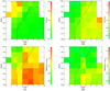 |
Fig. 5. Two-dimensional distribution of (a) Δl, (b) rAB, (c) maximum rA, and (d) minimum rA of the nonSSE blobs as a function of TS/N and DS/N when θSun is 135°. The black dashed lines mark the boundaries of the regions satisfying the inequality (6). |

The black lines in Fig. 4 mark the boundaries of regions satisfying the inequality (6). Based on the condition for S/N, we can estimate SS/N in the case of different θSun. For blobs of specific number density, SS/N is defined as the 3D space where the TS/N and DS/N of blobs satisfy the inequality (6). The volume of SS/N varies with the properties of synthetic blobs. Figure 6 displays SS/N in the COR-2 FOV with different θSun when the central number density of blobs is 5 × 104 cm−3 and 1.2 × 105 cm−3. In the case of 5 × 104 cm−3, SS/N excludes the space close to the inner edge on COR-2 images and passes through the meridian plane bisecting θSun. The variation of SS/N with θSun is faintly consistent with that of the 3D spatial distribution of low-density blobs of high reconstruction-quality levels (see Fig. 2). The SS/N of 1.2 × 105 cm−3 is closer to the overall COR-2 FOV, and so the 3D distribution of blobs of high density with good reconstruction quality is more extensive than those of low density. Furthermore, we calculate the volume of SS/N with different blob density (Fig. 7). Blobs with larger density are more likely to meet the S/N condition (6), and so SS/N has a larger volume. For blobs with number density smaller or larger than 4.5 × 104 cm−3, the volume of 135° or 150° is largest, respectively. Therefore, when θSun is 135°, there is more 3D space where low-density transients have suitable S/N for good reconstruction.
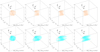 |
Fig. 6. Three-dimensional space that satisfies the inequality (6) when the number density of blobs is 5 × 104 cm−3 (panels a–d) and 1.2 × 105 cm−3 (panels e–h). θSun is 90° (panels a and e), 120° (panels b and f), 135° (panels c and g), and 150° (panel d and h). |
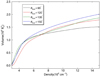 |
Fig. 7. Volume of SS/N as a function of the number density of blobs when θSun is 90° (black), 120° (red), 135° (green), and 150° (blue). |
4.2. The opening angle
In addition to the S/N of the images, the similarity between the transients on two images from different viewpoints also influences their reconstruction quality. This similarity is related to the opening angle (θblob), that is, the angle between lines connecting the transient and two spacecraft (see Fig. 1a). In the range of 90° −180°, the features of an optically thin transient on two images are more similar when θblob is closer to 180°. Transients with larger θblob are more likely to be identified, while the triangulation error is higher. For instance, the collinear effect is significant and transients are poorly reconstructed when the θblob of transients in the HI-1 FOV is close to 180° (Lyu et al. 2020). The range of θblob is positively related to θSun. For example, the range of θblob in the COR-2 FOV is about 112° −128° when θSun is 120° and about 142° −158° when θSun is 150°. It is important to study the suitable range of θblob of transients in the COR-2 FOV in order to find the optimal θSun for reconstruction.
We reconstruct nine blobs (Height: 8 R⊙, 10 R⊙, 12 R⊙; Latitude: −20°, 0°, 20°; Longitude: 0°) of the same radius, density, and velocity in 13 different cases of θSun (90° −150° in intervals of 5°) under the condition of Group 2. We find that the S/N of these blobs with the same properties and position varies very little with θSun, and the TS/N and DS/N of these blobs meet the inequality (6), meaning that the influence of variation in S/N on the reconstruction quality can be ignored. Figure 8 shows the variation of rAB as a function of the average θblob of blobs within the range of 90° −160°. As θblob increases, the half thickness rAB increases, which could explain the low frequency of Level-3 blobs in the context of 150° (Fig. 3). The blob with larger rAB is more distinguishable. Meanwhile, the expansion of reconstructed blobs with increasing θblob proves that the collinear effect also exists in the FOV of coronagraphs. To control the expansibility and the completeness of reconstructed transients, the best range of θblob is between 120° and 150°, which can be regarded as approximately a limit of suitable θSun for reconstruction.
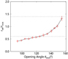 |
Fig. 8. rAB of blobs as a function of θblob. Blobs are of Group 2. |
4.3. Blob properties
Comparison of the WRQ of blobs of the four groups reveals that blobs with different properties may have different global reconstruction quality, and require different θSun for good-quality reconstruction. Therefore, we study the influence of the properties of blobs –including the number density, size, and velocity– on the global reconstruction quality.
Figure 9a shows the variation of the relative frequency of reconstruction quality levels as well as WRQ with the number density. When θSun is 135°, WRQ increases as the number density increases, because blobs have higher S/N on images and are more likely to be reconstructed (Fig. 9a). The slight decrease in WRQ with the number density larger than 105 cm−3 is related to the increasing rA and rB of reconstructed structures. This indicates that more unphysical structures may be reconstructed in the case of high density, and could explain why the number of high-density blobs at Level 3 is smaller than that of low-density blobs when θSun is 150° (Figs. 2d and h). According to Fig. 9a, we propose 0.8 − 1.2 × 105 cm−3 as the best range of number density for the detection and reconstruction of small-scale transients in the COR-2 FOV, although transients with higher density can also be accurately located and reconstructed.
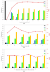 |
Fig. 9. Relative frequency of non-SSE blobs of different reconstruction-quality levels and WRQ (red line) as a function of the number density (panel a), the radius (panel b) and the 30-min movement in heliospheric distance (panel c) when θSun is 135°. The radial movement of 1 R⊙ in 30 min corresponds to the radial velocity about 390 km s−1. The colors representing different levels of reconstruction quality are the same as those in Fig. 2. |
Figure 9b shows the variation in frequency and WRQ with blob size. The diameter of blobs that is most suitable for the reconstruction is about 0.8−1.6 R⊙. Although WRQ is higher than 0.7, it is more difficult to accurately locate and reconstruct blobs with a radius of greater than 0.6 R⊙, which is possibly due to the increasing Δl and rAB of reconstructed structures. In previous studies, we found the collinear effect is more serious for large-scale CMEs (Lyu et al. 2021). The work in Liewer et al. (2011) also indicated that the errors from the DALE effect for reconstruction using the triangulation method may increase with the size of transients. Meanwhile, excessively small blobs may be poorly reconstructed due to the poor 3D resolution and low S/N. In general, variations in the size and density of blobs influence the global reconstruction quality of blobs, which leads to the difference in suitable θSun between nonSSE and SSE blobs shown in Fig. 3.
Slow solar-wind transients, such as blobs, normally propagate at velocities of less than 500 km s−1 (Sheeley et al. 1997, 2009; Sheeley & Rouillard 2010; López-Portela et al. 2018) in the heliosphere. The variation in WRQ with the movement of blobs in heliospheric distance from the Sun is shown in Fig. 9c. The radial movement of 1 R⊙ in a time interval of 30 min corresponds to a radial velocity of about 390 km s−1. We find that WRQ is always higher than 0.8 as the velocity increases. Considering the time resolution of COR-2 image data, the velocity variation has a minor impact on the reconstruction of small-scale transients in the slow solar wind.
5. Conclusion
To investigate the performance of the reconstruction method CORAR from coronagraph images with different θSun, that is, the angle between the lines connecting the Sun and two spacecraft, we applied the technique on synthetic blobs with different positions and properties, and studied the global reconstruction quality of blobs in the case of θSun > 90°. We find that the small-scale blobs studied here are of high global reconstruction quality when θSun is between 120° and 150°, and the optimal θSun for the reconstruction of small-scale coronal transients in the COR-2 FOV is close to 135°. These findings are in agreement with the range of optimal θSun in the HI-1 FOV (Lyu et al. 2020, 2021). We find that the optimal θSun is identical even though we adjust the conditions for assessing the reconstruction quality. Blobs located away from the meridian plane containing the Sun–Earth line and away from the inner edge on COR-2 images are more likely to be poorly reconstructed. For blobs of low density, their global reconstruction quality when θSun is 120° is smaller than that when θSun is 150°, which is different for blobs of high density. This indicates that the optimal θSun for high-density transients is smaller than that for low-density ones. In the case of θSun < 90°, the global reconstruction performance is similar to that for the case of (180° −θSun), and so the optimal θSun for reconstruction is close to 45°.
We also discuss the factors related to the range of suitable θSun for reconstruction, and the influence of blob properties on the reconstruction quality:
-
The position of blobs influences the distribution of the S/N of transients on COR-2 images. Blobs with higher magnitude and lower contrast of S/N on COR-2 images are of higher better reconstruction quality. When θSun is 135°, there are more 3D positions where low-density transients have suitable S/N for good reconstruction.
-
θblob, the opening angle between the lines connecting the transient and two spacecraft, should be 120° −150° for optimal reconstruction of blob shape, which limits the range of θSun suitable for reconstruction in the COR-2 FOV.
-
For small-scale transients on coronagraph images, their most suitable number density and size for reconstruction using the CORAR technique are 0.8 − 1.2 × 105 cm−3 and 0.8−1.6 R⊙, respectively, while transients of larger density and size may also be of good reconstruction quality. For slow-wind transients, the influence of velocity variation on reconstruction is subtle.
Combined with previous studies, the results of our tests can serve as a foundation for the current design of the SOlar Ring mission (Wang et al. 2023). The new scheme of three spacecraft can provide multi-view observations with θSun of 120° and 150° combined with observations from Earth. Moreover, the improved CORAR technique will be adjusted and applied not only to the real COR-2 images but also to images from other perspectives, such as LASCO on board SOHO, WISPR on board PSP, and SoloHI and Metis on board the Solar Orbiter in the future. We hope to study the evolution of real transients observed by multiple spacecraft with θSun suitable for the CORAR technique.
Acknowledgments
We acknowledge the use of the data from STEREO/SECCHI, which are produced by a consortium of RAL (UK), NRL (USA), LMSAL (USA), GSFC (USA), MPS (Germany), CSL (Belgium), IOTA (France), and IAS (France). The SECCHI data can be found in the STEREO Science Center (https://stereo-ssc.nascom.nasa.gov/data/ins_data/secchi/). We also acknowledge for the support from the National Space Science Data Center, National Science and Technology Infrastructure of China (http://www.nssdc.ac.cn). This work is supported by the National Natural Science Foundation of China (42188101, 41774178 and 42174213), the Strategic Priority Programs of the Chinese Academy of Sciences (XDB41000000 and XDA15017300), and the Informatization Plan of Chinese Academy of Sciences, Grant No. CAS-WX2021PY-0101. Y.W. is particularly grateful to the support of the Tencent Foundation.
References
- Balan, N., Skoug, R., Tulasi Ram, S., et al. 2014, J. Geophys. Res.: Space Phys., 119, 10,041 [NASA ADS] [Google Scholar]
- Bemporad, A., Pagano, P., & Giordano, S. 2018, A&A, 619, A25 [NASA ADS] [CrossRef] [EDP Sciences] [Google Scholar]
- Brueckner, G. E., Howard, R. A., Koomen, M. J., et al. 1995, Sol. Phys., 162, 357 [NASA ADS] [CrossRef] [Google Scholar]
- Colaninno, R. C., & Vourlidas, A. 2009, ApJ, 698, 852 [NASA ADS] [CrossRef] [Google Scholar]
- Davies, J. A., Harrison, R. A., Perry, C. H., et al. 2012, ApJ, 750, 23 [Google Scholar]
- Davies, J. A., Perry, C. H., Trines, R. M. G. M., et al. 2013, ApJ, 777, 167 [Google Scholar]
- de Koning, C. A., Pizzo, V. J., & Biesecker, D. A. 2009, Sol. Phys., 256, 167 [NASA ADS] [CrossRef] [Google Scholar]
- DeForest, C. E., Howard, T. A., & Tappin, S. J. 2013a, ApJ, 765, 44 [NASA ADS] [CrossRef] [Google Scholar]
- DeForest, C. E., Howard, T. A., & McComas, D. J. 2013b, ApJ, 769, 43 [NASA ADS] [CrossRef] [Google Scholar]
- DeForest, C. E., de Koning, C. A., & Elliott, H. A. 2017, ApJ, 850, 130 [NASA ADS] [CrossRef] [Google Scholar]
- DeForest, C. E., Howard, R. A., Velli, M., Viall, N., & Vourlidas, A. 2018, ApJ, 862, 18 [Google Scholar]
- Dere, K. P., Wang, D., & Howard, R. 2005, ApJ, 620, L119 [CrossRef] [Google Scholar]
- Domingo, V., Fleck, B., & Poland, A. I. 1995, Space Sci. Rev., 72, 81 [Google Scholar]
- Feng, L., Inhester, B., Wei, Y., et al. 2012, ApJ, 751, 11 [Google Scholar]
- Feng, L., Inhester, B., & Mierla, M. 2013, Sol. Phys., 282, 221 [NASA ADS] [CrossRef] [Google Scholar]
- Feng, L., Wang, Y., Shen, F., et al. 2015, ApJ, 812, 70 [NASA ADS] [CrossRef] [Google Scholar]
- Fox, N. J., Velli, M. C., Bale, S. D., et al. 2016, Space Sci. Rev., 204, 7 [Google Scholar]
- Gosling, J. T., Bame, S. J., McComas, D. J., & Phillips, J. L. 1990, Geophys. Res. Lett., 17, 901 [NASA ADS] [CrossRef] [Google Scholar]
- Harrison, R. A., Davis, C. J., & Eyles, C. J. 2005, Adv. Space Res., 36, 1512 [NASA ADS] [CrossRef] [Google Scholar]
- Horbury, T. S., Woolley, T., Laker, R., et al. 2020, ApJS, 246, 45 [Google Scholar]
- Howard, T. A., & DeForest, C. E. 2012, ApJ, 752, 130 [Google Scholar]
- Howard, T. A., Webb, D. F., Tappin, S. J., Mizuno, D. R., & Johnston, J. C. 2006, J. Geophys. Res.: Space Phys., 111, A04105 [NASA ADS] [CrossRef] [Google Scholar]
- Howard, R. A., Moses, J. D., Vourlidas, A., et al. 2008, Space Sci. Rev., 136, 67 [NASA ADS] [CrossRef] [Google Scholar]
- Howard, T. A., Tappin, S. J., Odstrcil, D., & DeForest, C. E. 2013, ApJ, 765, 45 [NASA ADS] [CrossRef] [Google Scholar]
- Howard, R. A., Vourlidas, A., Colaninno, R. C., et al. 2020, A&A, 642, A13 [NASA ADS] [CrossRef] [EDP Sciences] [Google Scholar]
- Hundhausen, A. J., Gilbert, H. E., & Bame, S. J. 1968, ApJ, 152, L3 [Google Scholar]
- Inhester, B. 2006, ArXiv e-prints [arXiv:astro-ph/0612649] [Google Scholar]
- Inhester, B. 2015, ArXiv e-prints [arXiv:1512.00651] [Google Scholar]
- Kaiser, M. L., Kucera, T. A., Davila, J. M., et al. 2008, Space Sci. Rev., 136, 5 [Google Scholar]
- Kasper, J. C., Bale, S. D., Belcher, J. W., et al. 2019, Nature, 576, 228 [Google Scholar]
- Ko, Y.-K., Fisk, L. A., Geiss, J., Gloeckler, G., & Guhathakurta, M. 1997, Sol. Phys., 171, 345 [NASA ADS] [CrossRef] [Google Scholar]
- Landi, E., Gruesbeck, J. R., Lepri, S. T., Zurbuchen, T. H., & Fisk, L. A. 2012, ApJ, 761, 48 [NASA ADS] [CrossRef] [Google Scholar]
- Li, X. L., Wang, Y. M., Liu, R., et al. 2018, J. Geophys. Res.: Space Phys., 123, 7257 [NASA ADS] [CrossRef] [Google Scholar]
- Li, X. L., Wang, Y., Liu, R., et al. 2020, J. Geophys. Res.: Space Phys., 125, e2019JA027513 [Google Scholar]
- Li, X. L., Wang, Y., Guo, J., Liu, R., & Zhuang, B. 2021, A&A, 649, A58 [NASA ADS] [CrossRef] [EDP Sciences] [Google Scholar]
- Liewer, P. C., Hall, J. R., Howard, R. A., et al. 2011, J. Atmos. Solar-Terr. Phys., 73, 1173 [NASA ADS] [CrossRef] [Google Scholar]
- Lugaz, N. 2010, Sol. Phys., 267, 411 [NASA ADS] [CrossRef] [Google Scholar]
- Lyu, S., Li, X., & Wang, Y. 2020, Adv. Space Res., 66, 2251 [Google Scholar]
- Lyu, S., Wang, Y., Li, X., et al. 2021, ApJ, 909, 182 [NASA ADS] [CrossRef] [Google Scholar]
- López-Portela, C., Panasenco, O., Blanco-Cano, X., & Stenborg, G. 2018, Sol. Phys., 293, 99 [Google Scholar]
- Manoharan, P. K. 2006, Sol. Phys., 235, 345 [NASA ADS] [CrossRef] [Google Scholar]
- Mierla, M., Davila, J., Thompson, W., et al. 2008, Sol. Phys., 252, 385 [NASA ADS] [CrossRef] [Google Scholar]
- Mierla, M., Inhester, B., Marque, C., et al. 2009, Sol. Phys., 259, 123 [NASA ADS] [CrossRef] [Google Scholar]
- Mierla, M., Inhester, B., Antunes, A., et al. 2010, Ann. Geophys., 28, 203 [NASA ADS] [CrossRef] [Google Scholar]
- Moestl, C., & Davies, J. A. 2013, Sol. Phys., 285, 411 [NASA ADS] [CrossRef] [Google Scholar]
- Moran, T. G., & Davila, J. M. 2004, Science, 305, 66 [Google Scholar]
- Moran, T. G., Davila, J. M., & Thompson, W. T. 2010, ApJ, 712, 453 [NASA ADS] [CrossRef] [Google Scholar]
- Morgan, H., Habbal, S. R., & Woo, R. 2006, Sol. Phys., 236, 263 [Google Scholar]
- Müller, D., St. Cyr, O. C., Zouganelis, I., et al. 2020, A&A, 642, A1 [Google Scholar]
- Pizzo, V. J., & Biesecker, D. A. 2004, Geophys. Res. Lett., 31, L21802 [Google Scholar]
- Sanchez-Diaz, E., Rouillard, A. P., Davies, J. A., et al. 2017a, ApJ, 851, 32 [Google Scholar]
- Sanchez-Diaz, E., Rouillard, A. P., Davies, J. A., et al. 2017b, ApJ, 835, L7 [Google Scholar]
- Sheeley, N. R., & Rouillard, A. P. 2010, ApJ, 715, 300 [NASA ADS] [CrossRef] [Google Scholar]
- Sheeley, N. R., Wang, Y. M., Hawley, S. H., et al. 1997, ApJ, 484, 472 [Google Scholar]
- Sheeley, N. R., Walters, J. H., Wang, Y. M., & Howard, R. A. 1999, J. Geophys. Res.: Space Phys., 104, 24739 [NASA ADS] [CrossRef] [Google Scholar]
- Sheeley, N. R., Lee, D. D. H., Casto, K. P., Wang, Y. M., & Rich, N. B. 2009, ApJ, 694, 1471 [NASA ADS] [CrossRef] [Google Scholar]
- Susino, R., Bemporad, A., & Dolei, S. 2014, ApJ, 790, 11 [CrossRef] [Google Scholar]
- Telloni, D., Zank, G. P., Stangalini, M., et al. 2022, ApJ, 936, L25 [NASA ADS] [CrossRef] [Google Scholar]
- Thernisien, A. F. R. 2011, ApJS, 194, 33 [NASA ADS] [CrossRef] [Google Scholar]
- Thernisien, A. F. R., Howard, R. A., & Vourlidas, A. 2006, ApJ, 652, 763 [Google Scholar]
- Thernisien, A. F. R., Vourlidas, A., & Howard, R. A. 2009, Sol. Phys., 256, 111 [NASA ADS] [CrossRef] [Google Scholar]
- Thompson, W. T. 2006, A&A, 449, 791 [NASA ADS] [CrossRef] [EDP Sciences] [Google Scholar]
- Viall, N. M., & Vourlidas, A. 2015, ApJ, 807, 176 [Google Scholar]
- Viall, N. M., DeForest, C. E., & Kepko, L. 2021, Front. Astron. Space Sci., 8, 139 [NASA ADS] [CrossRef] [Google Scholar]
- Volpes, L., & Bothmer, V. 2015, Sol. Phys., 290, 3005 [NASA ADS] [CrossRef] [Google Scholar]
- Vourlidas, A., & Howard, R. A. 2006, ApJ, 642, 1216 [Google Scholar]
- Vourlidas, A., Howard, R. A., Plunkett, S. P., et al. 2016, Space Sci. Rev., 204, 83 [Google Scholar]
- Wang, Y. M., Sheeley, J. N. R., Walters, J. H., et al. 1998, ApJ, 498, L165 [NASA ADS] [CrossRef] [Google Scholar]
- Wang, J.-J., Luo, B.-X., Liu, S.-Q., & Gong, J.-C. 2013, Chin. J. Geophys. Chin. Ed., 56, 2871 [Google Scholar]
- Wang, Y., Ji, H., Wang, Y., et al. 2020, Sci. China Technol. Sci., 63, 1699 [CrossRef] [Google Scholar]
- Wang, Y., Chen, X., Wang, P., et al. 2021, Sci. China Technol. Sci., 64, 131 [CrossRef] [Google Scholar]
- Wang, Y., Bai, X., Chen, C., et al. 2023, Adv. Space Res., 71, 1146 [NASA ADS] [CrossRef] [Google Scholar]
- Wiegelmann, T., Inhester, B., & Feng, L. 2009, Ann. Geophys., 27, 2925 [NASA ADS] [CrossRef] [Google Scholar]
- Xie, H., Ofman, L., & Lawrence, G. 2004, J. Geophys. Res.: Space Phys., 109, A03109 [NASA ADS] [Google Scholar]
- Xue, X. H., Wang, C. B., & Dou, X. K. 2005, J. Geophys. Res.: Space Phys., 110, A08103 [NASA ADS] [CrossRef] [Google Scholar]
- Zhao, X. P. 2008, J. Geophys. Res.: Space Phys., 113, A02101 [NASA ADS] [Google Scholar]
- Zhao, X. P., Plunkett, S. P., & Liu, W. 2002, J. Geophys. Res.: Space Phys., 107, SSH 13 [Google Scholar]
Appendix A: The auto-sampling CORAR technique
In step 2 of the CORAR method, we calculate the Pearson correlation coefficient (cc) of two projected images with a sampling box of constant size. The cc will have a high value in the position where transients exist, and the 3D high-cc space is recognized as the reconstructed structure of solar-wind transients. However, the sampling box with constant scale is unfit for coronal transients with various scales. Therefore, we developed an auto-sampling CORAR technique. For a selected pixel on images, we calculate the root mean square deviation of the values of the neighboring pixels from the value of the pixel closest to zero on the image. The deviation should be small if the pixel is in the regions without transients. We distinguish the regions containing transients on images if the deviation is larger than the threshold, adjust the sampling boxes for COR-2A and COR-2B images according to the size of transient regions, and output the overlapping area of two boxes as the final sampling area. Though images at three moments are input for reconstruction, we generate the sampling box according to the transients of the middle moment. For coronal transients, the improved technique can be used to detect and distinguish their multi-scale features more easily and completely. The structure of the synthetic blob reconstructed by the new auto-sampling method is more complete and accurate, especially for the central part, which may be ignored by the basic CORAR method (Fig. A.1).
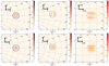 |
Fig. A.1. Reconstructed structure of a synthetic blob in the HEE X-Y plane (Panels a and d), X-Z plane (Panels b and e), and heliospheric surface (Panels c and f) containing the blob center. Panels (a)-(c): reconstruction using the CORAR technique with fixed sampling box. Panels (d)-(f): reconstruction using the auto-sampling CORAR technique. The blue circle masks the real blob size. The color bar shows the value of cc that represents the reconstructed structure. |
Appendix B: The case of θSun < 90°
To compare the reconstruction when θSun is smaller than and larger than 90°, we study the cases when θSun is 45° and 135° (Fig. B.1). The image features of the blob of 0° in HEE longitude when θSun is 45° is close to those of the blob of 90° when θSun is 135°, and so the reconstruction quality is similar. Likewise, the blob of k° in longitude when θSun is n° is of similar reconstruction quality to the blob of (k + 90)° when θSun is (180 − n)°. Therefore, the global reconstruction quality of transients in the COR-2 FOV is similar when θSun = n° and θSun = (180 − n)°. Figure B.2 presents the longitude profile of the relative frequency of blobs at different levels when θSun is 45° and 135°. It is evident that the distribution of the reconstruction quality in longitude when θSun = 45° has similar 180° periodicity to that when θSun = 135°, except for a 90° difference in longitude. Combined with the conclusion of the optimal θSun for reconstruction in the range of 90°-180°, the optimal θSun in the range of 0°-90° is close to 45°.
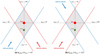 |
Fig. B.1. Common FOV of COR-2A and COR-2B, i.e., SCOR2, when θSun = 45° (Panel a) and θSun = 135° (Panel b). It is assumed that the lines of sight from the same observer are parallel. φHEE is the longitude in the HEE coordinate. |
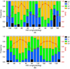 |
Fig. B.2. Relative frequency of nonSSE blobs at different levels and their WRQ (red line) as a function of HEE longitude. θSun is 45° (Panel a) and 135° (Panel b). There is a 90° difference between the ranges of HEE longitude in the two panels, and they display similar periods of 180° in longitude. |
All Tables
All Figures
|
Fig. 1. CORAR reconstruction of a synthetic blob. The location of the blob in the HEE coordinate is 0° in latitude, 30° in longitude, and 10 R⊙ in heliocentric distance. The number density at the center of the blob is about 3.5 × 104 cm−3. The separation angle between the Earth and the spacecraft STEREO-A/B is about 65°/71°. Panel a: coordinates of STEREO-A (STA), STEREO-B (STB), the Sun, and the synthetic blob. The STA-Sun-STB angle (θSun) and the STA-blob-STB angle (θblob, namely the opening angle in the text) are highlighted. LAB is defined as the connecting line of two spacecraft. Panel b: 3D presentation of the synthetic blob. Panels c and d: synthetic COR-2A and COR-2B images containing the blob. Panel e: 3D presentation of cc that represents the reconstructed structure (see the context in Sect. 2). Panel f: reconstructed structure in the X − Y plane. The half thickness rAB of the reconstructed structure in the direction of LAB is labeled. Panels g and h: reconstructed structure observed from the COR-2A and COR-2B perspectives. The maximum radii of the reconstructed blob on COR-2A and COR-2B images, i.e., maximum rA and rB, respectively, are labeled. |
| In the text | |
|
Fig. 2. Three-dimensional distributions of blobs at different levels of reconstruction quality in Group 1 (panels a–d), Group 2 (panels e–h), Group 3 (panels i–l), and Group 4 (panels m–p) when θSun is 90° (panels a, e, i, and m), 120° (panels b, f, j, and n), 135° (panels c, g, k, and o), and 150° (panels d, h, l, and p). See the descriptions of different groups in the text and Table 2. |
| In the text | |
|
Fig. 3. Relative frequency of blobs of different levels of reconstruction quality and their WRQ (red lines) with different θSun. The blobs are of Group 1 (panel a), Group 2 (panel b), Group 3 (panel c), and Group 4 (panel d). The colors representing different levels of reconstruction quality are the same as those in Fig. 2. |
| In the text | |
|
Fig. 4. Two-dimensional distribution of the WRQ of the nonSSE (panels a–d) and SSE (panels e–h) blobs as a function of TS/N and DS/N when θSun is 90° (panels a and e), 120° (panels b and f), 135° (panels c and g), and 150° (panels d and h). The black dashed lines mark the boundaries of the regions satisfying the inequality (6). |
| In the text | |
|
Fig. 5. Two-dimensional distribution of (a) Δl, (b) rAB, (c) maximum rA, and (d) minimum rA of the nonSSE blobs as a function of TS/N and DS/N when θSun is 135°. The black dashed lines mark the boundaries of the regions satisfying the inequality (6). |
| In the text | |
|
Fig. 6. Three-dimensional space that satisfies the inequality (6) when the number density of blobs is 5 × 104 cm−3 (panels a–d) and 1.2 × 105 cm−3 (panels e–h). θSun is 90° (panels a and e), 120° (panels b and f), 135° (panels c and g), and 150° (panel d and h). |
| In the text | |
|
Fig. 7. Volume of SS/N as a function of the number density of blobs when θSun is 90° (black), 120° (red), 135° (green), and 150° (blue). |
| In the text | |
|
Fig. 8. rAB of blobs as a function of θblob. Blobs are of Group 2. |
| In the text | |
|
Fig. 9. Relative frequency of non-SSE blobs of different reconstruction-quality levels and WRQ (red line) as a function of the number density (panel a), the radius (panel b) and the 30-min movement in heliospheric distance (panel c) when θSun is 135°. The radial movement of 1 R⊙ in 30 min corresponds to the radial velocity about 390 km s−1. The colors representing different levels of reconstruction quality are the same as those in Fig. 2. |
| In the text | |
|
Fig. A.1. Reconstructed structure of a synthetic blob in the HEE X-Y plane (Panels a and d), X-Z plane (Panels b and e), and heliospheric surface (Panels c and f) containing the blob center. Panels (a)-(c): reconstruction using the CORAR technique with fixed sampling box. Panels (d)-(f): reconstruction using the auto-sampling CORAR technique. The blue circle masks the real blob size. The color bar shows the value of cc that represents the reconstructed structure. |
| In the text | |
|
Fig. B.1. Common FOV of COR-2A and COR-2B, i.e., SCOR2, when θSun = 45° (Panel a) and θSun = 135° (Panel b). It is assumed that the lines of sight from the same observer are parallel. φHEE is the longitude in the HEE coordinate. |
| In the text | |
|
Fig. B.2. Relative frequency of nonSSE blobs at different levels and their WRQ (red line) as a function of HEE longitude. θSun is 45° (Panel a) and 135° (Panel b). There is a 90° difference between the ranges of HEE longitude in the two panels, and they display similar periods of 180° in longitude. |
| In the text | |
Current usage metrics show cumulative count of Article Views (full-text article views including HTML views, PDF and ePub downloads, according to the available data) and Abstracts Views on Vision4Press platform.
Data correspond to usage on the plateform after 2015. The current usage metrics is available 48-96 hours after online publication and is updated daily on week days.
Initial download of the metrics may take a while.