| Issue |
A&A
Volume 660, April 2022
|
|
|---|---|---|
| Article Number | A25 | |
| Number of page(s) | 14 | |
| Section | Astrophysical processes | |
| DOI | https://doi.org/10.1051/0004-6361/202142360 | |
| Published online | 04 April 2022 | |
Analytical techniques for polarimetric imaging of accretion flows in the Schwarzschild metric
1
Department of Physics and Astronomy, University of Turku, 20014 Turku, Finland
e-mail: This email address is being protected from spambots. You need JavaScript enabled to view it.
, This email address is being protected from spambots. You need JavaScript enabled to view it.
, This email address is being protected from spambots. You need JavaScript enabled to view it.
2
Nordita, KTH Royal Institute of Technology and Stockholm University, Hannes Alfvéns väg 12, 10691 Stockholm, Sweden
3
Space Research Institute of the Russian Academy of Sciences, Profsoyuznaya Str. 84/32, 117997 Moscow, Russia
Received:
3
October
2021
Accepted:
2
January
2022
Abstract
Emission from an accretion disk around compact objects, such as neutron stars and black holes, is expected to be significantly polarized. The polarization can be used to put constraints on the geometrical and physical parameters of the compact sources – their radii, masses, and spins – as well as to determine the orbital parameters. The radiation escaping from the innermost parts of the disk is strongly affected by the gravitational field of the compact object and the relativistic velocities of the matter. The straightforward calculation of the observed polarization signatures involves a computationally expensive ray-tracing technique. At the same time, having fast computational routines for direct data fitting is becoming increasingly important in light of the currently observed images of the accretion flow around the supermassive black hole in M 87 by the Event Horizon Telescope and infrared polarization signatures coming from Sgr A*, as well as the upcoming X-ray polarization measurements by the Imaging X-ray Polarimetry Explorer and enhanced X-ray Timing and Polarimetry mission. In this work, we obtain an exact analytical expression for the rotation angle of the polarization plane in the Schwarzschild metric accounting for the effects of light bending and relativistic aberration. We show that the calculation of the observed flux, polarization degree, and polarization angle as a function of energy can be performed analytically with a high level of accuracy using an approximate light-bending formula, eliminating the need for the precomputed tabular models in fitting routines.
Key words: accretion, accretion disks / galaxies: active / gravitational lensing: strong / methods: analytical / polarization / stars: black holes
© ESO 2022
1. Introduction
Accretion disks around compact objects – neutron stars (NSs) and black holes (BHs) – are among the most efficient energy conversion engines in the Universe. As the matter spirals in towards the compact object, it releases the excess of gravitational energy via radiation. Understanding of the physical mechanisms leading to energy liberation and geometrical properties of the emitting medium is an important goal of the modern high-energy astrophysics. Recent investigations have been focused on the innermost parts of the accretion disk in the regime of strong gravity. X-ray spectroscopy (Reynolds 2014; Bambi et al. 2021) and timing techniques (Revnivtsev et al. 1999; Gilfanov et al. 2003; Uttley et al. 2014; Axelsson & Veledina 2021) have been exploited to trace the geometry of the inner parts of the accretion flow and to identify contributions of various components that are emitting in the X-ray energy range.
Polarimetry is known to be a fine measure of the geometry and radiative processes operating in the accretion flow. Numerous efforts are being aimed at predicting and finding distinct signatures of the accretion disk in a strong gravity regime from the polarimetric information (e.g., Dovčiak et al. 2008; Li et al. 2009; Ingram et al. 2015). Polarimetry in the infrared and millimeter bands was recently shown to be a powerful tool for studying the structure of accretion flows in the vicinity of supermassive BHs in the Milky Way (GRAVITY Collaboration 2018; Bower et al. 2018) and in M 87 (Event Horizon Telescope Collaboration 2021a,b). For studies of NSs and stellar-mass BHs, radiating mostly in the X-ray range, the full capacity of polarimetry will be used with the upcoming launch of dedicated satellites, such as Imaging X-ray Polarimetry Explorer (IXPE, Weisskopf et al. 2021) and enhanced X-ray Timing and Polarimetry mission (eXTP, Zhang et al. 2019). For the BH X-ray binaries, in the absence of a solid surface of the compact object, accretion is the only source of the observed X-ray emission, and the obtained signatures can be directly connected to the innermost geometry of the accretion disk. For the NS X-ray binaries, such as accreting millisecond pulsars, the disk can serve as a source of constant energy-dependent polarimetric background, which has to be subtracted to obtain polarimetric profiles of pulsations (Viironen & Poutanen 2004).
Rees (1975) discussed the polarimetric signatures of the accretion disks with the dominant role of electron scattering (Chandrasekhar 1960; Sobolev 1963) in the Newtonian approximation. Observing such polarization signatures has been considered crucial for confirming the existence of an accretion disk in the first place (Lightman & Shapiro 1975). A number of deviations from this simple model were discussed, such as the role of true absorption, for which Monte-Carlo estimates have been presented by Lightman & Shapiro (1975) and the analytic results are discussed in Loskutov & Sobolev (1979) and Loskutov & Sobolev (1981), along with the alignment of the inner parts of the disk with the BH spin (Bardeen & Petterson 1975).
Yet another important addition to the early works on the disk polarization signatures is inclusion of the effects of special and general relativity (GR and SR; Connors & Stark 1977; Stark & Connors 1977; Pineault & Roeder 1977a,b). Relativistic aberration and light deflection lead to a rotation of the polarization angle (PA) and alter the viewing angle of different segments of the disk, the latter effect leading to a different polarization degree (PD) of a given segment; while the PD is Lorentz invariant, the difference with respect to the non-relativistic case appears because of the different angle between the disk normal and the observer direction. Frame dragging effects, relevant to spinning BHs described by Kerr (1963) metric, lead to the additional rotation of the polarization plane along the photon trajectory. Calculations of all these effects involve the parallel transport of the polarization vector along null geodesics, which requires calculations of the Walker & Penrose (1970) constant of motion. For every null geodesics leaving the disk, the polarization at infinity can be evaluated by solving linear equations for the components of the polarization vector (e.g., Connors & Stark 1977; Connors et al. 1980; Dovčiak et al. 2008; Li et al. 2009; Ingram et al. 2015).
In this implicit formulation, the calculation of Stokes parameters is related to the computationally expensive numerical integration of the equation of geodesic, known as the ray-tracing technique. With the launch of X-ray polarimetric satellites, the data fitting procedures will require fast routines for calculating the polarization from accretion disks. A high time gain can be achieved, for instance, by tabulating the observed polarization characteristics of the disk rings for different BH and orbit parameters, so that the minimization routines would only need to proceed via interpolation between the precomputed models. On the other hand, the tabulated models would have to be recalculated with any change to the local model, such as an alteration of the angular dependence of emission or radial energy dissipation profile. Similar problems are faced within the analysis and theoretical modeling of polarimetric images of accretion flows around supermassive BHs. To accelerate the calculations, Narayan et al. (2021) recently developed a fast code for evaluating polarimetric images in Schwarzschild metric, which is based on evaluation of Walker-Penrose constants and an approximation of the light bending formula from Beloborodov (2002). Understanding the role of different relativistic effects and their separation in the total image, however, remains elusive, as explicit analytical expressions for the PA and PD transformation – as a result of the joint action of GR and SR – have not been presented thus far.
Using such explicit formulae to directly relate the local and the observed PA and PD can also substantially speed up the minimization routine. Connors et al. (1980) give an explicit analytical expression for the rotation angle of the polarization plane due to solely SR effects (their Eq. (18)). Pineault (1977) pointed out that the total rotation of PA in Schwarzschild metric and after accounting for relativistic motions in the disk is not a simple sum of rotations caused by the relativistic motion in the flat space ( ) and the light bending (χGR).
In this work, we derive explicit analytical expressions for the rotation of the PA accounting for the relativistic motion of matter in the accretion disk and light bending in Schwarzschild metric. Corresponding formulae were previously derived for polarization properties of rapidly rotating NSs (Viironen & Poutanen 2004; Poutanen 2020a; Loktev et al. 2020). We use the laws of geometrical optics and exploit the fact that the light trajectories are flat in Schwarzschild metric, that is, the orientation of the polarization vector is fixed with respect to the angular momentum of the ray trajectory (see Pineault 1977). The light bending is computed using the recent analytical approximation derived in Poutanen (2020b), which allows us to achieve high accuracy, with the deviations from the exact solution being smaller than the existing or expected statistical errors of observations. This removes the need for using computationally expensive ray-tracing algorithms when computing the polarization of the accretion disks around NSs or low-spin BHs.
2. Polarized radiation from the accretion disk
2.1. Observed flux
We consider the emission of a disk surface element in an axially symmetric, geometrically (infinitely) thin accretion disk in Schwarzschild metric. We compute the observed Stokes parameters following the approach described in Poutanen (2020b) and repeat here the basic notations and formulae for completeness.
We choose a Cartesian coordinate system with the z-axis coinciding with the normal to the disk and x-axis lying along with the projection of the line of sight on the disk (see Fig. 1). In this system, the normal to the disk  , the unit vector in the observer direction
  , and the radius-vector of the surface element
  have the following coordinates:
 (1)
(1)
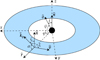 |
Fig. 1. Geometry of a flat accretion disk ring. The emitting surface element is described by the radius-vector r and velocity v. Vector |

where φ is the azimuth of the radius-vector measured from the x-axis and i is the disk inclination to the line of sight. The radius-vector of the surface element makes angle ψ to the line of sight:
 (2)
(2)
The photon trajectories are planar in Schwarzschild metric, hence, the direction of the photon momentum close to the disk surface can be described as a linear combination of the observer vector and the radius-vector of the emission point:
![Mathematical equation: $$ \begin{aligned} \hat{\boldsymbol{k}}_0 = [\sin \alpha \, \hat{\boldsymbol{o}} + \sin (\psi -\alpha )\, \hat{\boldsymbol{r}}]/\sin \psi , \end{aligned} $$](/articles/aa/full_html/2022/04/aa42360-21/aa42360-21-eq8.gif) (3)
(3)
where
 (4)
(4)
The relation between the angles α and ψ is described by the light-bending integral or can be approximated using a simple analytical formula (Pechenick et al. 1983; Beloborodov 2002; Poutanen & Beloborodov 2006; Salmi et al. 2018; Poutanen 2020b).
We consider purely Keplerian motion of disk matter, with the velocity unit vector being parallel to the azimuthal vector:
 (5)
(5)
The dimensionless velocity, β = v/c, relative to a static observer at the circumferential radius, r = R/RS, measured in units of the Schwarzschild radius RS = 2GM/c2 of the central object of mass M, is (see e.g., Luminet 1979):
 (6)
(6)
where u = 1/r is the compactness. The corresponding Lorentz factor is
 (7)
(7)
The photon momentum makes angle ξ with the velocity vector:
 (8)
(8)
and angle ζ with the disk normal,
 (9)
(9)
The Doppler factor is:
 (10)
(10)
The unit vector of the photon momentum in the frame comoving with the surface element (fluid frame hereafter) is computed using Lorentz transformation:
![Mathematical equation: $$ \begin{aligned} \hat{\boldsymbol{k}}^{\prime }_0 = \delta \left[\hat{\boldsymbol{k}}_0 - \gamma \beta \hat{\boldsymbol{v}} + (\gamma -1) \hat{\boldsymbol{v}} (\hat{\boldsymbol{v}}\cdot \hat{\boldsymbol{k}}_0)\right]. \end{aligned} $$](/articles/aa/full_html/2022/04/aa42360-21/aa42360-21-eq16.gif) (11)
(11)
From this, we get the angle between the photon momentum and the local normal in the fluid frame
 (12)
(12)
The projection of the photon momentum on the disk plane in that frame has azimuth ϕ′ (as measured from the radial direction) and can be determined through:
 (13)
(13)
 (14)
(14)
Specific flux observed from the surface element at photon energy E is:
 (15)
(15)
where dΩ is the solid angle occupied by the surface element on the observer’s sky, IE is the specific intensity of radiation at infinity, which is related to the intensity in the fluid frame:
 (16)
(16)
Here, we assume that I′ does not depend on the azimuthal angle ϕ′ and for brevity omit its dependence on radius r. The total redshift factor (Luminet 1979; Chen et al. 1989),
 (17)
(17)
combines the effects of the gravitational redshift and the Doppler effect. The solid angle occupied by the surface element of area  is given by:
 (18)
(18)
Here, dS cos ζ is the projection of the element area on the plane of the sky, D is the distance to the source and
 (19)
(19)
is the lensing factor (Beloborodov 2002; Poutanen 2020b). We obtain the final expression for the observed spectral flux in the form:
 (20)
(20)
The total observed flux from the disk can then be obtained by integrating Eq. (20) over the radius and azimuthal angle:
 (21)
(21)
For a chosen inclination i and for every pair (r, φ), we compute ψ using Eq. (2), which is then used to compute α and ℒ – either exactly from elliptical integrals (as described, e.g., in Salmi et al. 2018), or using analytical formulae (see Poutanen 2020b and Sect. 2.4). Then, ξ and ζ are obtained from Eqs. (8) and (9), respectively. Using the Keplerian velocity and the Lorentz factor given by Eqs. (6) and (7), we then get the Doppler factor δ from Eq. (10). Further, from Eqs. (12) and (17), we get the photon energy E′ and the zenith angle ζ′ in the fluid frame, which are needed to obtain  and, if needed, the azimuth ϕ′ from Eqs. (13) and (14).
2.2. Computing polarized flux
We consider only the linear polarization, which is described by the three-component Stokes vector1. The direction of the polarization vector changes along the photon trajectory because of the gravitational light bending and aberration. The key property of the Schwarzschild metric that allows us to derive simple analytical formulae for the PA rotation is that the angle between the polarization vector and the trajectory plane is conserved.
In order to describe polarized radiation in the fluid frame, it is convenient to introduce the polarization basis formed by the vector of the local normal and the photon momentum  :
:
 (22)
(22)
The radiation field emitted at angle ζ′ from the disk surface with coordinates (r, φ) is then described by the Stokes vector
 (23)
(23)
where p is the linear PD of radiation, which is invariant, namely, it does not change along photon trajectory. The PA χ0 is defined as the angle between the polarization vector and the basis vector  measured in the counterclockwise direction. The transformation of vector
  to the observed Stokes vector involves rotation by the corresponding Mueller matrix:
 (24)
(24)
where χtot is the rotation angle of the polarization plane. Combining this matrix with Eq. (20), we get the expression for the observed Stokes vector (in terms of fluxes):
 (25)
(25)
Integrating over azimuth and radius, we get the observed Stokes vector from the entire disk surface:
 (26)
(26)
If the angular distribution of radiation escaping from the disk surface (as measured in the fluid frame) does not depend on the azimuth ϕ′, but only on the zenith angle ζ′, the polarization vector is parallel to one of the basis vectors (22) and the Stokes U-parameter vanishes, namely, χ0 = 0 or π/2. Equation (25) is transformed to:
 (27)
(27)
Integrating over r and φ, we easily get the total observed Stokes vector. We note that the transformation of the Stokes vectors does not depend on the nature of radiation escaping from the disk or on the assumption about the direction of the polarization vector in the fluid frame; it is fully determined by the rotation of the polarization plane, χtot. In order to obtain an analytical solution relating the emitted and observed Stokes vectors, we need to find an explicit formula for χtot.
2.3. Polarization angle
Here, we consider the physical reasons for the rotation of the polarization plane. The polarization vector is determined by the predominant direction of the electric field oscillations. The angle the polarization vector makes with respect to the projection of the disk normal,  , on the plane perpendicular to the photon trajectory is called the polarization angle (PA). As the photon propagates to the observer, the polarization vector remains perpendicular to the direction of motion. The light bending imposes changes to the photon propagation direction. In the Schwarzschild metric, each trajectory lies in a plane, and the normal to this plane remains the same along the whole trajectory. Hence, the polarization vector rotates around the normal to the trajectory plane. In a general case, the normal to the trajectory plane does not coincide with the disk normal,
  , hence, the angle between the polarization vector and
  changes. Accordingly, this causes changes in the PA.
The Lorentz transformation between the lab frame and the fluid frame also constitutes a rotation of the photon momentum vector, and the polarization vector rotates correspondingly. As long as the normal  is not the axis of the rotation, the PA acquires additional rotation.
The PA seen by the observer is the sum of the PA of emitted photon and its total rotation along the trajectory:
 (28)
(28)
The PA rotation can be computed directly from the rotation of the polarization plane and the projection of the polarization vector onto the sky, as viewed by the observer. The rotation by the general relativistic (GR) light bending effects is (see derivation in Appendix A.2):
 (29)
(29)
where
 (30)
(30)
This expression accounts only for GR (light bending) effects, while in reality the matter in the disk moves around the compact object at relativistic velocities, hence we need to account also for the SR effects, namely, for the relativistic aberration.
If the surface element moves at a velocity  , the photon vector,
  , as measured in the observers (static) frame, is related to the vector
  , as measured in the fluid frame, via the Lorentz transformation. This transformation leads to the additional rotation of the PA, which can be written as (see Appendix A.3 for derivation)
 (31)
(31)
We note that this expression takes into account the fact that the photon reaching the observer experiences light bending and, hence, the outgoing photon in the static reference frame close to the disk surface propagates along with the vector  – and not
  .
.
For the case of a flat space, when α = ψ, the expression above is reduced to:
 (32)
(32)
which is equivalent to Eq. (18) of Connors et al. (1980) for the case of the disk polarization perpendicular to meridional plane made by the photon momentum and the local normal, namely, χ0 = π/2.
The total rotation of the PA is the sum of two rotations (Eqs. (29) and (31)):
 (33)
(33)
This expression is different from the simple addition of rotations due to light bending, χGR, and rotation in flat space,  (Eq. (32)), as originally noted in Pineault (1977). The reason for this is that the Lorentz transformation has to be applied to the photon momentum after accounting for the bending effect.
2.4. Light bending
The formulae presented above allow us to directly transform the Stokes parameters of radiation escaping from the surface element to the observed ones. To obtain the complete analytical transformation, we need to have an expression for α(ψ, r). The exact integral equation for the inverse function, ψ(α, r) (Pechenick et al. 1983; Beloborodov 2002; Poutanen 2020b), can be used to compute the original expression at high accuracy. For this, the function ψ(α, r) has to be tabulated at a dense grid of arguments and then the function α(ψ, r) can be obtained by interpolation (Salmi et al. 2018).
Alternatively, an approximate analytical expression (Beloborodov 2002) can be used:
 (34)
(34)
where y = 1 − cos ψ. This approximation gives ℒ = 1 for the lensing factor in Eq. (19). This relation was recently used in Narayan et al. (2021) to compute polarized images of an accretion disk in Schwarzschild metric observed nearly face-on. The approximate relation (34) is accurate only when ψ ≲ 90° and therefore cannot be used for high inclinations.
Higher accuracy can be achieved by using the recently proposed relation (Poutanen 2020b):
![Mathematical equation: $$ \begin{aligned} \cos \alpha \approx 1 - y(1-u) \left\{ 1+\frac{u^2y^2}{112}-\frac{euy}{100} \left[\ln \left(1-\frac{y}{2}\right)+\frac{y}{2}\right]\right\} , \end{aligned} $$](/articles/aa/full_html/2022/04/aa42360-21/aa42360-21-eq55.gif) (35)
(35)
where e is the base of natural logarithm. This relation can also be used for high inclinations. In particular, this relation gives a relative accuracy in α better than 0.06% at ψ < 120° and any radius exceeding 1.5 RS. At these radii, the error does not exceed 0.2% for ψ < 162° (which is valid for any azimuthal angle φ and inclinations of i < 72°). Using Eq. (35), we get a similarly accurate analytical representation for the lensing factor:
![Mathematical equation: $$ \begin{aligned} {\mathcal{L} } \approx 1 + \frac{3u^2y^2}{112} - \frac{e}{100} u y \left[2\, \ln \left(1-\frac{y}{2}\right) + y\frac{1-3y/4}{1-y/2}\right]\cdot \end{aligned} $$](/articles/aa/full_html/2022/04/aa42360-21/aa42360-21-eq56.gif) (36)
(36)
Equations (35) and (36) can be used instead of the exact relations for fast and accurate calculations of the observed Stokes parameters, as well as the polarized images.
2.5. Images
The formalism developed above allows us to obtain images of the accretion disk on the sky in polarized light. For any point on the disk with polar coordinates (r, φ), we first compute the angle between the observer direction and the radius vector of the element ψ using Eq. (2). Then, using either exact or approximate relations for light bending, we get angle α, which is then used to get the impact parameter in units of RS (Pechenick et al. 1983; Beloborodov 2002):
 (37)
(37)
Owing to the fact that photon trajectories are planar is Schwarzschild metric, we get the position angle Φ (measured counterclockwise from the projection of the disk axis on the sky) of the point where photon hits the plane of the sky:
 (38)
(38)
 (39)
(39)
The error on b is fully determined by the accuracy of the relation α(ψ), while Φ is exact.
3. Applications
In this section, we show examples of calculations of the observed polarization signatures affected by the GR and SR effects. We start with the simple decomposition of the action of these effects on the PA rotation (χGR and χSR). We then proceed to a comparison between PA rotations obtained using the exact and approximate α(ψ) relations. This relation is also used when obtaining the angle of the outgoing photon to the disk normal, which ultimately affects the observed flux and PD. Finally, we show the calculations of the polarization signatures of the geometrically thin, optically thick (Shakura & Sunyaev 1973; Novikov & Thorne 1973) accretion disk.
3.1. Stokes vector for a narrow ring
Relativistic effects on polarization are expected to be of the highest importance at the smallest disk radii. First, we consider radiation produced at the radius of r = 3, corresponding to the innermost stable circular orbit for a Schwarzschild BH. In Fig. 2, we show the angles χSR, χGR, and χtot as a function of azimuth in the disk for different system inclinations. We define PA in the range [− 90° ;90°]. In general, both the GR and SR rotations decrease with increasing inclination. This leads to higher depolarizing effects at smaller inclinations, which is a known result (Dovčiak et al. 2008).
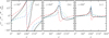 |
Fig. 2. Rotation angles of the polarization plane, χGR (red dot-dashed lines), χSR (blue dashed lines), |

The curve χGR (red dot-dashed in Fig. 2) is (anti-)symmetric with respect to the azimuth φ = 0° and 180°. For r = 3, the rotation is highest at  . The position of the extrema can be obtained analytically if we apply the Beloborodov (2002) approximation for the light-bending angle to the expression (29) for the rotation angle (see Appendix A.2 for derivation):
 (40)
(40)
This approximation gives  .
.
The SR effects are computed for the Keplerian rotation given by Eq. (6). The curve χSR (blue dashed curve in Fig. 2) is not symmetric, which adds to the asymmetry of the total PA rotation χtot. At sufficiently large inclinations, χSR has a maximum very close to φ = 180°. Interestingly, the shape of the similar curve in flat space,  , is very different (compare dashed blue with dotted green curves). In flat space, the maximum rotation angle is reached at (see Eq. (32)):
 (41)
(41)
Obviously, the extrema do not exist if β > sin i and then  is monotonic. A general formula for the rotation angle χSR does not allow us to obtain a simple analytical expression for the position of the extrema. We note that the numerator of Eq. (31) is a smooth function of φ, therefore, the rotation angle reaches maximum close to the azimuth where the denominator reaches minimum:
 (42)
(42)
By noticing that the corresponding azimuth is close to 180° and that α and ψ vary slowly with φ, and putting ψ ≈ 90° +i, we get:
 (43)
(43)
where we can substitute cos α = u − (1 − u) sin i using Beloborodov (2002) approximation for the light-bending angle. For r = 3 and i = 60° (80°), the exact calculations give the maximum at  (
( ), while Eq. (43) gives
  (
( ).
).
The total rotation, χtot, is shown with the black solid lines in Fig. 2. Notably, for inclinations of i ≲ 30°, the PA rotation is monotonic with azimuth and crosses 90°. This means that the polarization direction significantly changes, making two full cycles as the azimuth varies from 0 to 360°. Although in Fig. 2a, we see that only χSR makes two cycles, the total effect is not entirely caused by the relativistic rotation. Namely, for small inclinations, all the light rays coming to the observer were originally emitted along the direction of radius-vectors, that is,  , for any azimuth. It means that the observer sees the ring from its outer parts as if every disk element was located between the observer and the BH in the flat space. This is taken into account in χSR, when we apply Lorentz transformation to these rays. The direction of matter motion, with respect to the observer, varies between these disk segments, leading to variations of the angles between vectors
  and
and  . Hence, the SR effects only enhance the PA rotation caused by the light bending. If GR effects alone do not cause the full rotation of PA (such as in Fig. 2a), the additional rotation coming from relativistic motion results in the crossing of the 90° boundary. For the same reason, we see two full rotations of PA for the case when the bright spot orbits the BH. For inclination 180° −i, both the GR and SR rotation angles change sign.
In Fig. 3, we show the total PA rotation χtot for different radii and inclinations, as well as the error on the PA computed using the analytical expression for light bending (35), as compared to the exact, numerical solution. We see that the relativistic effects decrease with radius, as expected. The largest rotation of the PA is observed at smaller inclinations. The difference between the PA computed using analytical formulae and numerically is always smaller than  .
.
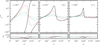 |
Fig. 3. Upper panels: PA χtot as a function of azimuth for disk inclinations i = 30° (a), 60° (b) and 80° (c) and different r = 3 (black solid line), 5 (red dashed), 15 (green dot-dashed) and 50 (blue dotted). Lower panels: difference in the PA rotation computed using analytical formula (35) for light bending and via the exact calculations. |
The topology of χtot is shown in Fig. 4 as a map on the accretion disk plane in the form of contours of constant values. It is similar to that shown in Fig. 3 of Dovčiak et al. (2008), but defined here on the range of angles [− 90° ,90°] (rather than the previously used [− 180° ,180°], which included two full cycles of PA). We see that for i = 30°, there exists a critical point (at r ≈ 4.06, φ ≈ 230°) where photons are emitted along the disk normal in the comoving frame (i.e., ζ′ = 0) resulting in zero PD and not defined PA. At large inclinations, the strongest variations in PA are seen around φ = 180°. Calculations using the analytical formula for light bending produce nearly identical pictures (see the dotted lines barely separable from the solid lines in Fig. 4).
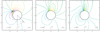 |
Fig. 4. Contours of constant χtot at the accretion disk plane (r, φ). The observer is situated at inclinations i = 30° (panel a), 60° (panel b), and 80° (panel c). The coordinates are in units of RS. The polar angle φ is measured from the projection of the direction to the observer on the disk plane. The disk rotates in the counterclockwise direction. The innermost stable circular orbit at r = 3 is shown with a black circle. The dotted lines (wherever visible) show corresponding contours computed using the approximate formula for light bending (35). |
The general topology of χtot is easier to understand by looking separately at the topology of χGR and χSR, which are presented in Figs. 5 and 6, respectively. The anti-symmetry of χGR in φ and very small rotation angles around φ ≈ 0 are clearly seen. Also at φ ≈ 180° the GR rotation is small at large radii, while closer to r = 3, the contours of constant values become highly packed, corresponding to very fast changes of PA with azimuth. At small inclinations the GR rotation of PA is large, while, for instance, at i = 80°, significant rotation happens only close to φ = 180°. For the χSR, we see the existence of the critical point at small inclinations outside r = 3. The peak in SR rotation is reached close to φ = 180° and the effect of SR rotation decreases with the increasing inclination, similarly to the GR rotation angle.
Interestingly, in the specific case of zero inclination i = 0, the expressions for the GR and the SR rotation angles can be considerably simplified:
 (44)
(44)
 (45)
(45)
resulting in the total rotation:
 (46)
(46)
Using Beloborodov (2002) approximation and assuming Keplerian rotation, we further get:
 (47)
(47)
For r → ∞, this transforms to χSR(r, i = 0) = φ − π/2. This is different by π from the expression for the rotation angle in flat space given by Eq. (32) in the limit i → 0:
 (48)
(48)
that is, both limits give the same position angle of the polarization (pseudo-)vector. On the other end, at the innermost stable orbit, r = 3, according to Eq. (47) the PA rotates by  (exact calculations give
  ).
).
Light bending and aberration do not only rotate the polarization plane but also affect the flux and PD, as they alter the angle at which we see the surface element. In Fig. 7 we show, for the photon reaching the observer, the zenith angle ζ′ between the local normal and photon propagation direction in the fluid frame, as well as the difference between the angles computed numerically and using approximate analytical formula (35). This angle differs from the observer inclination i, because of the light bending and aberration. The photon rays originating in the parts of the disk behind the BH (around φ = 180°) experience the most pronounced bending, because the light trajectory lies above the BH at closer distances than the emission radius. This results in pronounced dips in ζ′ (seen in Fig. 7c), where the disk is seen more face-on (i.e. ζ′< i). The SR effects make the surface seen more face-on at places, where matter moves towards the observer, that is, φ > 180° and otherwise more edge-on for φ < 180°, where the matter of the disk moves away from the observer. This effect is noticeable for moderate and low inclinations, thus, the change of ζ′ in Fig. 7a is mainly due to SR effects. The error in ζ′, when using the approximate bending formula, grows with inclination, but the largest difference is still below  (for i = 80°, see Fig. 7c).
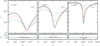 |
Fig. 7. Upper panels: zenith angle ζ′ the photon reaching the observer makes to the local normal in the fluid frame as a function of the azimuth for disk inclinations i = 30° (panel a), 60° (b), and 80° (c) and different emission radii r = 3 (black solid line), 5 (red dashed), 15 (green dot-dashed), and 50 (blue dotted). Lower panels: difference between ζ′ computed using the analytical formula (35) for light bending and the one using exact formula. |
There is a general decrease with regard to the importance of GR and SR effects with increasing distance from the BH, hence, the difference between the PAs computed using exact and approximate lensing formulae decreases with radius (Fig. 3a). However, counter-intuitively, as we see in Figs. 7b and c that the error in ζ′ grows with the radius of the ring around azimuthal angle φ = 180°. For high disk inclination, the impact parameter of photons propagating towards the observer – as well as the distance of closest approach to the central compact object – are much smaller than the radius of the corresponding ring. This leads to a larger, although still within  , inaccuracy in ζ′ for the approximation formula at high inclinations.
In Fig. 8, we show the quantity g3ℒ cos ζ, which is proportional to the observed flux from a surface element (see Eq. (20)). Here, we clearly see the effect of Doppler boosting for part of the ring at φ > 180° and deboosting for φ < 180°. For a high-inclination observer, gravitational lensing strongly amplifies the flux from the part of the disk behind the BH at φ ∼ 180°. The azimuthal dependence of the flux is not symmetric because of the increasing role of the Doppler boosting towards φ ∼ 270°. The relative error on the flux arising from the approximate bending and lensing formulae is largest for high inclinations, at azimuths of φ ∼ 180°, when the angle ψ is large. The largest error at r = 3 reaches 26% for i = 80°, while for i = 30° and 60°, it does not exceed 0.6%.
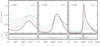 |
Fig. 8. Upper panels: combination g3ℒ cos ζ which is proportional to the observed flux from a disk surface element as a function of the azimuth for inclinations i = 30° (a), 60° (b), and 80° (c) and different emission radii r = 3 (black solid line), 5 (red dashed), 15 (green dot-dashed), and 50 (blue dotted). Lower panels: relative error (in %) on that combination computed using analytical formulae (35) and (36) for the light bending angle and lensing factor as compared to the exact calculations. |
3.2. Polarization of accretion disk in the Schwarzschild metric
We compute the polarization signatures of the optically thick, geometrically (infinitely) thin accretion disk using the analytical formulae derived above. The intensity of the disk in the fluid frame depends on the radius r, energy E′, and the angle ζ′ between the photon vector and the disk normal,  . As an illustration, we consider the simple case of the standard accretion disk in Newtonian gravity (Shakura & Sunyaev 1973) and pure electron scattering atmosphere for polarization properties. Substituting relevant dependencies in Eq. (23), we obtain the Stokes vector in the fluid frame:
 (49)
(49)
where
 (50)
(50)
approximates the angular dependence of the outgoing intensity (Suleimanov et al. 2020),
 (51)
(51)
approximates the angular dependence of the PD, and the PA of χ0 = π/2 is used corresponding to the direction of the polarization vector perpendicular to the meridional plane (Chandrasekhar & Breen 1947; Chandrasekhar 1960; Sobolev 1949, 1963).
The spectral shape is described by the Planck function BE′ of the color temperature, Tc = fcTeff, with the color correction factor assumed to be fc = 1.7 (Shimura & Takahara 1995). For the radial dependence of the effective temperature, we use a simple expression for a standard Newtonian disk (Shakura & Sunyaev 1973):
 (52)
(52)
where
 (53)
(53)
![Mathematical equation: $$ \begin{aligned}&t (u)=\left[u^3\left(1-\sqrt{3u}\right)\right]^{1/4}. \end{aligned} $$](/articles/aa/full_html/2022/04/aa42360-21/aa42360-21-eq92.gif) (54)
(54)
Figure 9 shows images of the accretion disk as viewed at three different inclinations. The colors reflect the bolometric intensity, which is given by the product g4t4(u)aes(ζ′). The black and white contours represent the sky images of lines of equal radii r and equal azimuths φ, computed using exact bending relation and its approximation (35), respectively. The difference is only visible for i ≥ 60° at the accretion disk side behind the black hole, φ ≈ 180°, corresponding to ψ ≈ 150° −170° and photon trajectories lying close to the black hole. We also plot the polarization pseudo-vectors. The green sticks correspond to the exact calculations, while the blue one to the approximate light bending formula. The PA and PD are nearly identical for these two cases, as they are defined by χtot and ζ′, which are very well approximated by the analytical formulae (see Figs. 4 and 7). Small inaccuracy of the light bending formula leads to minor differences in the positions of the sticks on the plane of the sky, while the difference in their angles (PA) and lengths (PD) cannot be seen by eye.
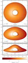 |
Fig. 9. Images of an accretion disk as viewed at three inclinations i = 30° (a), 60° (b), and 80° (c). The coordinates on the sky are given in units of RS. Contours show the images of rings of equal radii r (from 3 to 15, with a step of 3) and equal azimuths φ (every 30°). Black solid contours correspond to the exact calculations of α(ψ), while the white dashed contours (almost fully overlapping with the black ones) are for the approximation (35). The colors reflect the logarithm of g4t4(u)aes(ζ′), which is proportional to the bolometric intensity. The blue sticks give polarization computed using approximate light bending expression (35), with their length being proportional to the PD and their position angle is given by the PA. Exact calculations shown by green sticks are nearly indistinguishable from the approximation. |
Using Eqs. (26) and (27), we integrate over radius and azimuth to get the observed Stokes vector. The Stokes vector of the apparent luminosity is computed by multiplying the Stokes vector FE by 4πD2. The luminosity can be represented in a dimensionless form by scaling it to  , multiplying by photon energy and using the dimensionless photon energy x = E/kT* as an argument:
![Mathematical equation: $$ \begin{aligned} x \boldsymbol{l}_x =&\frac{x \boldsymbol{L}_x}{\sigma _{\rm SB}T_*^4R_{\rm S}^2} = \frac{60}{\pi ^4} \int \limits _{r_{\rm in}}^{r_{\rm out}}\!\! \frac{r \,\mathrm{d}r}{\sqrt{1-u}} \int _0^{2\uppi } \mathrm{d}\varphi \, \frac{g^4}{f_{\rm c}^4}\ \mathcal{L} \,\cos \zeta \nonumber \\&\times \frac{x^{\prime 4} a_{\rm es}(\zeta^\prime )}{\mathrm{e}^{\displaystyle x\prime /f_{\rm c}t(u)}-1} \begin{bmatrix} 1\\ p_{\rm es}(\zeta^\prime ) \cos (2[\chi ^\mathrm{tot}+\chi _0]) \\ p_{\rm es}(\zeta^\prime ) \sin (2[\chi ^\mathrm{tot}+\chi _0]) \end{bmatrix}, \end{aligned} $$](/articles/aa/full_html/2022/04/aa42360-21/aa42360-21-eq94.gif) (55)
(55)
where x = gx′. With such scaling of photon energy and luminosity, spectra of accretion disk become independent of the BH mass and accretion rate.
The positively defined observed PD is then
 (56)
(56)
The observed PA is computed as an argument of the complex quantity formed by the Stokes parameters:
 (57)
(57)
In Fig. 10, we show the resulting spectral energy distributions of x lx, PD (p) and PA (χ) for the accretion disk extending from rin = 3 to rout = 3000 in the Schwarzschild metric, as seen by a distant observer at different inclinations: i = 30°, 60°, and 80°. Figure 10a shows the dimensionless luminosity as a function of photon energy at three inclinations. It is much higher at low inclinations due to the strong beaming of radiation along with the normal in the electron-scattering dominated atmosphere. At higher inclinations, the Doppler effects shift the peak of emission to higher energies. The lower subpanel shows the relative error on luminosity when computations are done using approximate formulae for the light-bending angle (35) and lensing factor (36). In spite of the fact that the error on the lensing factor reaches nearly 30% at r = 3 for i = 80° (see Fig. 8), the integral flux has at most 1.5% relative error, owing to the fact that the error in ℒ at different radii has a different sign.
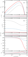 |
Fig. 10. Polarized spectrum of a standard accretion disk (3 < r < 3000) viewed at different inclinations: i = 30° (red solid line), 60° (blue dashed), 80° (black dotted) as a function of dimensionless photon energy x = E/kT*. Panel a: normalized luminosity x lx. Panel b: polarization degree. Panel c: polarization angle. The lower subpanels show the errors in the corresponding quantities when computations are done with approximate expressions Eqs. (35) and (36) for the bending angle and lensing factor. We note that the error on x lx is relative, while the errors on PA and PD are absolute. |
The PD (see Fig. 10b) is much higher for high inclinations. At lower energies, the emission is dominated by large radii where relativistic effects are not important and PD follows the angular dependence given by p(i)≈pes(ζ′). In agreement with previous findings (Stark & Connors 1977; Connors et al. 1980; Dovčiak et al. 2008), we observe the increase of the value of the rotation angle and the increasing role of depolarization effects at higher energies (see Figs. 10b and c), where the emission from the innermost radii is most important. Because the observed flux is dominated (due to the Doppler effect) by the part of the disk at φ ≈ 270°, where the rotation angle is large, the integrated rotation angle is high at small inclinations. The range of rotation angles is wide in this case (see Figs. 2–4), hence the depolarization effect is strongest at higher energies. As described, for example, in Dovčiak et al. (2008), the recovery of PD at energies higher than kT* is caused by the fact that only a small area of the disk contributes to this range of energies and, therefore, the depolarizing effects are smaller. Calculations using approximate formulae for light bending and lensing factor give very accurate results in these cases, too. For example, the absolute error on PD is smaller than 0.03% for all inclinations and the error on the PA barely exceeds  .
.
Our calculations of one image shown in Fig. 9 were performed in 0.01 s when using the approximate analytical formula, while the calculations of one polarized spectrum from Fig. 10 take about 0.05 s. Similar calculations using interpolation in table α(ψ, r) obtained from the exact implicit formula for ψ(α, r) took about 1 s. On the other hand, direct calculations using a ray-tracing code ARCMANCER (Pihajoki et al. 2018) took about 103 s to compute an image 400 × 400 pixels.
3.3. Extensions of the model
The fully analytical formalism developed above can naturally be applied to a number of problems on the production of polarized radiation near relativistic objects. First, the assumption that radiation is produced in a plane-parallel electron-scattering atmosphere can be relaxed. In this specific model, the Stokes vector defined in a polarization basis connected to the local normal contains only two non-zero parameters: I and Q. Properties of the local emission can be very different in other setups. For example, the accretion flows around BHs at low accretion rates are optically thin and polarization at low photon energies (radio to sub-millimeter for super-massive BHs and optical–infrared for X-ray binaries) may be related to synchrotron radiation of relativistic electrons (Poutanen & Veledina 2014; Yuan & Narayan 2014). The magnetic field direction in this situation will not likely be aligned with the local normal. In this case, the Stokes vector will contain three (or four, if we also consider circular polarization) components. In the X-ray domain, the PD and PA may also be very different from the optically thick case, as the photons are produced by Comptonization in a geometrically thick, optically thin hot flow. However, these deviations will change only the Stokes vector of the radiation escaping the disk, but will not affect the computational scheme of the observed polarized flux Stokes vector, which still will follow Eq. (26), with the expressions for the PA rotation angle remaining the same.
Another extension of the model is related to the velocity field of the accreting matter. In this paper, we assume that the gas velocity has only the azimuthal component, while, for example, an optically thin hot flow at low accretion rates, as seen by the EHT in M 87, may have a significant radial component (Event Horizon Telescope Collaboration 2021a,b; Narayan et al. 2021). We note that rotation of the polarization plane due to light bending χGR does not depend at all on the velocity field. To calculate the rotation χSR caused by special relativity effects in this case, we can use a more general expression (A.27) in the vector form.
A further extension of the model concerns the properties of the polarized flux if the emission is confined to a small region (hot spots) corotating with the flow (e.g., Pineault 1977; Connors et al. 1980). In this case, Eq. (25) for the observed Stokes vector as a function of emission azimuthal angle φ should be modified to account for the light travel time delays. It will depend on the photon arrival time (corresponding to the phase of the orbit, φobs):
 (58)
(58)
where dS′ is the emission region area in the fluid frame, which is now multiplied by cos ζ′, instead of cos ζ. The relation between the emission azimuth φ and the arrival time can be obtained from the time delay integral (see e.g., Pechenick et al. 1983; Poutanen & Beloborodov 2006; Salmi et al. 2018).
4. Summary
In this work, we derive explicit analytical expressions describing the rotation of the polarization plane in Schwarzschild metric. We show that the total rotation is a sum of two effects: the rotation caused by the light bending (Eq. (29)), which is a pure GR effect, and the relativistic aberration. The latter effect acts on the PA in a way that is different from the relativistic aberration in flat space, because it has to be applied to the photons whose path will subsequently be altered by the bending (Eq. (31)).
We show test cases for the observed PA from a disk ring, as a function of azimuth for various emission radii and observer inclinations. In combination with the recently derived analytical formula for the light bending, it is possible to compute both the zenith angle of emission in the fluid frame (that will affect the observed flux and PD) and PA with an accuracy better than 1° for any inclination and emission radius. This opens up a possibility to produce high-precision polarized images of the accretion disks in the Schwarzschild metric in an unprecedentedly small computing time.
Integration over the disk surface gives the full observed Stokes vector as a function of energy. Utilizing the analytical formulae allows reducing the computing time compared to the ray-tracing calculations by a factor of a hundred giving accuracy better than 1% on the flux, 0.03% on the integrated PD, and about  for the PA. Our analytical technique can be used for a detailed comparison of theoretical models with the polarimetric data on accretion disks around NSs and BHs.
The fourth component describing circular polarization is affected by light bending and aberration exactly the same way as the intensity, I, and the circular polarization degree is conserved along photon trajectory in the absence of plasma effects.
Acknowledgments
This research (specifically in Sect. 3.2) was supported by the Russian Science Foundation grant 20-12-00364. We also acknowledge support from the Jenny and Antti Wihuri foundation (VL) and the Academy of Finland grants 309308 (AV), 322779 and 333112 (JP).
References
- Axelsson, M., & Veledina, A. 2021, MNRAS, 507, 2744 [NASA ADS] [CrossRef] [Google Scholar]
- Bambi, C., Brenneman, L. W., Dauser, T., et al. 2021, Space Sci. Rev., 217, 65 [CrossRef] [Google Scholar]
- Bardeen, J. M., & Petterson, J. A. 1975, ApJ, 195, L65 [Google Scholar]
- Beloborodov, A. M. 2002, ApJ, 566, L85 [Google Scholar]
- Bower, G. C., Broderick, A., Dexter, J., et al. 2018, ApJ, 868, 101 [NASA ADS] [CrossRef] [Google Scholar]
- Chandrasekhar, S. 1960, Radiative Transfer (New York: Dover) [Google Scholar]
- Chandrasekhar, S., & Breen, F. H. 1947, ApJ, 105, 435 [NASA ADS] [CrossRef] [Google Scholar]
- Chen, K., Halpern, J. P., & Filippenko, A. V. 1989, ApJ, 339, 742 [NASA ADS] [CrossRef] [Google Scholar]
- Connors, P. A., & Stark, R. F. 1977, Nature, 269, 128 [Google Scholar]
- Connors, P. A., Piran, T., & Stark, R. F. 1980, ApJ, 235, 224 [Google Scholar]
- Dovčiak, M., Muleri, F., Goosmann, R. W., Karas, V., & Matt, G. 2008, MNRAS, 391, 32 [CrossRef] [Google Scholar]
- Event Horizon Telescope Collaboration (Akiyama, K., et al.) 2021a, ApJ, 910, L12 [Google Scholar]
- Event Horizon Telescope Collaboration (Akiyama, K., et al.) 2021b, ApJ, 910, L13 [Google Scholar]
- Gilfanov, M., Revnivtsev, M., & Molkov, S. 2003, A&A, 410, 217 [NASA ADS] [CrossRef] [EDP Sciences] [Google Scholar]
- GRAVITY Collaboration (Abuter, R., et al.) 2018, A&A, 618, L10 [NASA ADS] [CrossRef] [EDP Sciences] [Google Scholar]
- Ingram, A., Maccarone, T. J., Poutanen, J., & Krawczynski, H. 2015, ApJ, 807, 53 [NASA ADS] [CrossRef] [Google Scholar]
- Kerr, R. P. 1963, Phys. Rev. Lett., 11, 237 [Google Scholar]
- Li, L.-X., Narayan, R., & McClintock, J. E. 2009, ApJ, 691, 847 [CrossRef] [Google Scholar]
- Lightman, A. P., & Shapiro, S. L. 1975, ApJ, 198, L73 [NASA ADS] [CrossRef] [Google Scholar]
- Loktev, V., Salmi, T., Nättilä, J., & Poutanen, J. 2020, A&A, 643, A84 [NASA ADS] [CrossRef] [EDP Sciences] [Google Scholar]
- Loskutov, V. M., & Sobolev, V. V. 1979, Astrofizika, 15, 241 [NASA ADS] [Google Scholar]
- Loskutov, V. M., & Sobolev, V. V. 1981, Astrofizika, 17, 97 [NASA ADS] [Google Scholar]
- Luminet, J. P. 1979, A&A, 75, 228 [Google Scholar]
- Narayan, R., Palumbo, D. C. M., Johnson, M. D., et al. 2021, ApJ, 912, 35 [NASA ADS] [CrossRef] [Google Scholar]
- Novikov, I. D., & Thorne, K. S. 1973, in Black Holes (Les Astres Occlus), eds. C. DeWitt, & B. DeWitt (New York: Gordon and Breach), 343 [Google Scholar]
- Pechenick, K. R., Ftaclas, C., & Cohen, J. M. 1983, ApJ, 274, 846 [Google Scholar]
- Pihajoki, P., Mannerkoski, M., Nättilä, J., & Johansson, P. H. 2018, ApJ, 863, 8 [Google Scholar]
- Pineault, S. 1977, MNRAS, 179, 691 [Google Scholar]
- Pineault, S., & Roeder, R. C. 1977a, ApJ, 212, 541 [NASA ADS] [CrossRef] [Google Scholar]
- Pineault, S., & Roeder, R. C. 1977b, ApJ, 213, 548 [NASA ADS] [CrossRef] [Google Scholar]
- Poutanen, J. 2020a, A&A, 641, A166 [NASA ADS] [CrossRef] [EDP Sciences] [Google Scholar]
- Poutanen, J. 2020b, A&A, 640, A24 [NASA ADS] [CrossRef] [EDP Sciences] [Google Scholar]
- Poutanen, J., & Beloborodov, A. M. 2006, MNRAS, 373, 836 [NASA ADS] [CrossRef] [Google Scholar]
- Poutanen, J., & Veledina, A. 2014, Space Sci. Rev., 183, 61 [CrossRef] [Google Scholar]
- Rees, M. J. 1975, MNRAS, 171, 457 [NASA ADS] [CrossRef] [Google Scholar]
- Revnivtsev, M., Gilfanov, M., & Churazov, E. 1999, A&A, 347, L23 [NASA ADS] [Google Scholar]
- Reynolds, C. S. 2014, Space Sci. Rev., 183, 277 [Google Scholar]
- Salmi, T., Nättilä, J., & Poutanen, J. 2018, A&A, 618, A161 [NASA ADS] [CrossRef] [EDP Sciences] [Google Scholar]
- Shakura, N. I., & Sunyaev, R. A. 1973, A&A, 24, 337 [NASA ADS] [Google Scholar]
- Shimura, T., & Takahara, F. 1995, ApJ, 445, 780 [Google Scholar]
- Sobolev, V. V. 1949, Uch. Zap. Leningrad Univ., 16 [Google Scholar]
- Sobolev, V. V. 1963, A Treatise on Radiative Transfer (Princeton: Van Nostrand) [Google Scholar]
- Stark, R. F., & Connors, P. A. 1977, Nature, 266, 429 [NASA ADS] [CrossRef] [Google Scholar]
- Suleimanov, V. F., Poutanen, J., & Werner, K. 2020, A&A, 639, A33 [NASA ADS] [CrossRef] [EDP Sciences] [Google Scholar]
- Uttley, P., Cackett, E. M., Fabian, A. C., Kara, E., & Wilkins, D. R. 2014, A&ARv, 22, 72 [NASA ADS] [CrossRef] [Google Scholar]
- Viironen, K., & Poutanen, J. 2004, A&A, 426, 985 [NASA ADS] [CrossRef] [EDP Sciences] [Google Scholar]
- Walker, M., & Penrose, R. 1970, Commun. Math. Phys., 18, 265 [NASA ADS] [CrossRef] [Google Scholar]
- Weisskopf, M. C., Soffitta, P., Baldini, L., et al. 2021, ArXiv e-prints [arXiv:2112.01269] [Google Scholar]
- Yuan, F., & Narayan, R. 2014, ARA&A, 52, 529 [NASA ADS] [CrossRef] [Google Scholar]
- Zhang, S., Santangelo, A., Feroci, M., et al. 2019, Sci. China Phys. Mech. Astron., 62, 29502 [Google Scholar]
Appendix A: Rotation of the polarization plane
A.1. Rotation of PA for two polarization bases
For a photon moving along a unit vector  , we can define a polarization basis of two unit vectors perpendicular to each other as well as to
  as:
as:
 (A.1)
(A.1)
where l is an arbitrary vector not collinear with  . The angle the polarization plane of such a photon makes with the vector
  measured counterclockwise as viewed by the observer defines the polarization angle (PA) of the photon in this basis.
Two bases,  and
and  , built around the same photon vector
  , differ only by rotation around
  by an angle
  (see Fig. A.1) that may be defined by trigonometric functions as:
 (A.2)
(A.2)
 (A.3)
(A.3)
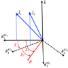 |
Fig. A.1. Polarization bases, |


In this case, the PA (i.e., position angle of the electric vector of a photon moving along  ) in basis 1 can be computed from the PA in basis 2 as χ1 = χ2 + χ. The angle χ can be expressed through its tangent
 (A.4)
(A.4)
A.2. Rotation of PA due to light bending
We go on to quantify the effect of the gravitational light bending only. We assume that the Stokes vector of emitted radiation is defined at the disk surface in the lab (non-rotating) frame in the basis related to the disk normal  , that is,
  . On the other hand, the observer defines PA in the basis formed by
  and the photon momentum at infinity
  , that is,
  . The way to find the rotation of the polarization plane between those two bases is to note that photon trajectories are flat in the Schwarzschild metric and the polarization vector is parallel transported along the trajectory. Since the photon trajectory plane is defined by the vectors
  and
and  (as well as
  ), the PA measured in bases
  and
and  is the same. Thus, the GR effect on PA consists of two terms only. The first one is the rotation of the polarization vector due to transformation from the basis
  to
to  , that is,
  . The second one is the rotation angle
  from basis
  to
to  . The total effect is then
 (A.5)
(A.5)
where
 (A.6)
(A.6)
 (A.7)
(A.7)
where we used the facts that  ,
,  and
and  , with the rest of scalar products obtained directly from Eqs. (1)–(5):
 (A.8)
(A.8)
 (A.9)
(A.9)
 (A.10)
 (A.11)
 (A.12)
 (A.13)
We thus get the tangent of the sum of the two rotation angles
![Mathematical equation: $$ \begin{aligned} \tan \chi ^{\mathrm{GR} }&= \tan \left(\chi (\hat{\boldsymbol{k}}_0,\hat{\boldsymbol{n}} \rightarrow \hat{\boldsymbol{r}}) +\chi (\hat{\boldsymbol{o}},\hat{\boldsymbol{r}} \rightarrow \hat{\boldsymbol{n}}) \right)\nonumber \\&= -\frac{(\cos \alpha -\cos \psi )(\hat{\boldsymbol{o}} \cdot \hat{\boldsymbol{\varphi }})(\hat{\boldsymbol{o}} \cdot \hat{\boldsymbol{n}})}{\cos \alpha \cos \psi (\hat{\boldsymbol{o}} \cdot \hat{\boldsymbol{n}})^2 + (\hat{\boldsymbol{o}} \cdot \hat{\boldsymbol{\varphi }})^2}\nonumber \\&=\frac{-(\hat{\boldsymbol{o}} \cdot \hat{\boldsymbol{\varphi }})(\hat{\boldsymbol{o}} \cdot \hat{\boldsymbol{n}})}{\tilde{a}[1-(\hat{\boldsymbol{o}} \cdot \hat{\boldsymbol{n}})^2]+(\hat{\boldsymbol{o}}\cdot \hat{\boldsymbol{r}})}\nonumber \\&=\frac{\cos i\sin \varphi }{\tilde{a}\sin i+\cos \varphi }, \end{aligned} $$](/articles/aa/full_html/2022/04/aa42360-21/aa42360-21-eq144.gif) (A.14)
(A.14)
where
 (A.15)
and we used the relation between directional cosines
 (A.16)
We see that χGR = 0 at φ = 0 where it changes the sign. Using Beloborodov (2002) approximation for the light bending angle, cos α = u + (1 − u) cos ψ, we get
 (A.17)
which allows us to obtain a simple approximate expression for the rotation angle due to the light bending only:
 (A.18)
The extrema are reached at
 (A.19)
This approximation works whenever the absolute value of the right-hand-side of Eq. (A.19) is smaller than unity; for instance, for r = 3, the inclination should be i > 30°. For r = 3 and i = 60°, the extrema appear at  , i.e. at φext, B02 ≈ 180° ∓16°, corresponding to
  (or
(or  ), while the exact calculations give
  and
and  .
.
A.3. Rotation of PA due to aberration
Next we consider the effect of the special relativity (SR) on the PA. In the local frame, we assume the element of the disk symmetric with respect to the local normal vector to the disk surface,  . Therefore, the properties of the outgoing radiation in the local frame are only defined by the angle it makes with the vertical direction. An atmosphere model under such an assumption would give the polarization vector in
  to be collinear to one of the basis vectors. The rotation of PA due to aberration can be decomposed into three rotations. First, from the basis
  to
to  . Second, from
  to
to  . Third, from
  to
to  . We note that the second rotation is actually zero, because the three vectors
  , and
, and  lie in the same plane, with the photon momenta unit vectors connected via the Lorenz transformation (11). Thus, the total rotation of the PA due to the SR may be written as:
 (A.20)
Noting that  , each angle can be computed using Eq. (A.4):
 (A.21)
 (A.22)
Using the relation  valid in our case, and expression (11) for the Lorentz transformation, we get
 (A.23)
 (A.24)
The tangent of the sum of two angles is then
![Mathematical equation: $$ \begin{aligned} \tan \chi ^{\mathrm{SR} }&= \frac{(\hat{\boldsymbol{k}}_0 \cdot \hat{\boldsymbol{r}}) (\hat{\boldsymbol{k}}_0^\prime \cdot \hat{\boldsymbol{n}})(\hat{\boldsymbol{k}}_0^\prime \cdot \hat{\boldsymbol{v}}) -(\hat{\boldsymbol{k}}_0^\prime \cdot \hat{\boldsymbol{r}}) (\hat{\boldsymbol{k}}_0 \cdot \hat{\boldsymbol{v}}) (\hat{\boldsymbol{k}}_0 \cdot \hat{\boldsymbol{n}})}{(\hat{\boldsymbol{k}}_0^\prime \cdot \hat{\boldsymbol{n}}) (\hat{\boldsymbol{k}}_0^\prime \cdot \hat{\boldsymbol{v}}) (\hat{\boldsymbol{k}}_0 \cdot \hat{\boldsymbol{n}}) (\hat{\boldsymbol{k}}_0 \cdot \hat{\boldsymbol{v}}) + (\hat{\boldsymbol{k}}_0^\prime \cdot \hat{\boldsymbol{r}}) (\hat{\boldsymbol{k}}_0 \cdot \hat{\boldsymbol{r}})}\nonumber \\&= \frac{(\hat{\boldsymbol{k}}_0 \cdot \hat{\boldsymbol{r}})(\hat{\boldsymbol{k}}_0 \cdot \hat{\boldsymbol{n}}) \left[(\hat{\boldsymbol{k}}_0 \cdot \hat{\boldsymbol{v}} - \beta ) - (1-\beta \hat{\boldsymbol{k}}_0\cdot \hat{\boldsymbol{v}}) (\hat{\boldsymbol{k}}_0 \cdot \hat{\boldsymbol{v}}) \right]}{(\hat{\boldsymbol{k}}_0 \cdot \hat{\boldsymbol{v}} - \beta ) (\hat{\boldsymbol{k}}_0 \cdot \hat{\boldsymbol{v}}) (\hat{\boldsymbol{k}}_0 \cdot \hat{\boldsymbol{n}})^2 + (1-\beta \hat{\boldsymbol{k}}_0\cdot \hat{\boldsymbol{v}}) (\hat{\boldsymbol{k}}_0 \cdot \hat{\boldsymbol{r}})^2}\nonumber \\&= \frac{\beta (\hat{\boldsymbol{k}}_0 \cdot \hat{\boldsymbol{r}})(\hat{\boldsymbol{k}}_0 \cdot \hat{\boldsymbol{n}}) \left((\hat{\boldsymbol{k}}_0 \cdot \hat{\boldsymbol{v}})^2-1\right)}{(\hat{\boldsymbol{k}}_0 \cdot \hat{\boldsymbol{v}})^2 (\hat{\boldsymbol{k}}_0 \cdot \hat{\boldsymbol{n}})^2 + (\hat{\boldsymbol{k}}_0 \cdot \hat{\boldsymbol{r}})^2 -\beta (\hat{\boldsymbol{k}}_0\cdot \hat{\boldsymbol{v}}) \left[(\hat{\boldsymbol{k}}_0 \cdot \hat{\boldsymbol{r}})^2+(\hat{\boldsymbol{k}}_0 \cdot \hat{\boldsymbol{n}})^2\right]}\nonumber \\&= - \frac{\beta (\hat{\boldsymbol{k}}_0 \cdot \hat{\boldsymbol{r}})(\hat{\boldsymbol{k}}_0 \cdot \hat{\boldsymbol{n}})}{1-(\hat{\boldsymbol{k}}_0 \cdot \hat{\boldsymbol{n}})^2-\beta (\hat{\boldsymbol{k}}_0\cdot \hat{\boldsymbol{v}})} = -\beta \,\frac{\cos \alpha \cos \zeta }{\sin ^2\zeta -\beta \cos \xi }, \end{aligned} $$](/articles/aa/full_html/2022/04/aa42360-21/aa42360-21-eq172.gif) (A.25)
(A.25)
where we used the relation for the directional cosines
 (A.26)
In flat space, we substitute α = ψ, ζ = i, cos ξ = − sin i sin φ and obtain Eq. (32).
In a more general case, when vectors  , and
, and  do not form the orthonormal basis, the expression for tanχSR becomes somewhat more cumbersome. However, if the velocity is perpendicular to the normal vector (with relation to which we measure the PA in the first place), that is,
  , then the rotation angle can still be written in a manner similar to the penultimate expression of Eq. (A.25):
 (A.27)
All Figures
|
Fig. 1. Geometry of a flat accretion disk ring. The emitting surface element is described by the radius-vector r and velocity v. Vector |
| In the text | |
|
Fig. 2. Rotation angles of the polarization plane, χGR (red dot-dashed lines), χSR (blue dashed lines), |
| In the text | |
|
Fig. 3. Upper panels: PA χtot as a function of azimuth for disk inclinations i = 30° (a), 60° (b) and 80° (c) and different r = 3 (black solid line), 5 (red dashed), 15 (green dot-dashed) and 50 (blue dotted). Lower panels: difference in the PA rotation computed using analytical formula (35) for light bending and via the exact calculations. |
| In the text | |
|
Fig. 4. Contours of constant χtot at the accretion disk plane (r, φ). The observer is situated at inclinations i = 30° (panel a), 60° (panel b), and 80° (panel c). The coordinates are in units of RS. The polar angle φ is measured from the projection of the direction to the observer on the disk plane. The disk rotates in the counterclockwise direction. The innermost stable circular orbit at r = 3 is shown with a black circle. The dotted lines (wherever visible) show corresponding contours computed using the approximate formula for light bending (35). |
| In the text | |
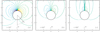 |
Fig. 5. Same as Fig. 4, but for χGR. |
| In the text | |
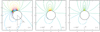 |
Fig. 6. Same as Fig. 4, but for χSR. |
| In the text | |
|
Fig. 7. Upper panels: zenith angle ζ′ the photon reaching the observer makes to the local normal in the fluid frame as a function of the azimuth for disk inclinations i = 30° (panel a), 60° (b), and 80° (c) and different emission radii r = 3 (black solid line), 5 (red dashed), 15 (green dot-dashed), and 50 (blue dotted). Lower panels: difference between ζ′ computed using the analytical formula (35) for light bending and the one using exact formula. |
| In the text | |
|
Fig. 8. Upper panels: combination g3ℒ cos ζ which is proportional to the observed flux from a disk surface element as a function of the azimuth for inclinations i = 30° (a), 60° (b), and 80° (c) and different emission radii r = 3 (black solid line), 5 (red dashed), 15 (green dot-dashed), and 50 (blue dotted). Lower panels: relative error (in %) on that combination computed using analytical formulae (35) and (36) for the light bending angle and lensing factor as compared to the exact calculations. |
| In the text | |
|
Fig. 9. Images of an accretion disk as viewed at three inclinations i = 30° (a), 60° (b), and 80° (c). The coordinates on the sky are given in units of RS. Contours show the images of rings of equal radii r (from 3 to 15, with a step of 3) and equal azimuths φ (every 30°). Black solid contours correspond to the exact calculations of α(ψ), while the white dashed contours (almost fully overlapping with the black ones) are for the approximation (35). The colors reflect the logarithm of g4t4(u)aes(ζ′), which is proportional to the bolometric intensity. The blue sticks give polarization computed using approximate light bending expression (35), with their length being proportional to the PD and their position angle is given by the PA. Exact calculations shown by green sticks are nearly indistinguishable from the approximation. |
| In the text | |
|
Fig. 10. Polarized spectrum of a standard accretion disk (3 < r < 3000) viewed at different inclinations: i = 30° (red solid line), 60° (blue dashed), 80° (black dotted) as a function of dimensionless photon energy x = E/kT*. Panel a: normalized luminosity x lx. Panel b: polarization degree. Panel c: polarization angle. The lower subpanels show the errors in the corresponding quantities when computations are done with approximate expressions Eqs. (35) and (36) for the bending angle and lensing factor. We note that the error on x lx is relative, while the errors on PA and PD are absolute. |
| In the text | |
|
Fig. A.1. Polarization bases, |
| In the text | |
Current usage metrics show cumulative count of Article Views (full-text article views including HTML views, PDF and ePub downloads, according to the available data) and Abstracts Views on Vision4Press platform.
Data correspond to usage on the plateform after 2015. The current usage metrics is available 48-96 hours after online publication and is updated daily on week days.
Initial download of the metrics may take a while.