| Issue |
A&A
Volume 650, June 2021
|
|
|---|---|---|
| Article Number | L9 | |
| Number of page(s) | 5 | |
| Section | Letters to the Editor | |
| DOI | https://doi.org/10.1051/0004-6361/202141274 | |
| Published online | 15 June 2021 | |
Letter to the Editor
Cumulene carbenes in TMC-1: Astronomical discovery of l-H2C5⋆
1
Grupo de Astrofísica Molecular, Instituto de Física Fundamental (IFF-CSIC), C/ Serrano 121, 28006 Madrid, Spain
e-mail: carlos.cabezas@csic.es, jose.cernicharo@csic.es
2
Observatorio Astronómico Nacional (IGN), C/ Alfonso XII, 3, 28014 Madrid, Spain
3
Centro de Desarrollos Tecnológicos, Observatorio de Yebes (IGN), 19141 Yebes, Guadalajara, Spain
Received:
8
May
2021
Accepted:
31
May
2021
We report the first detection in space of the cumulene carbon chain l-H2C5. A total of eleven rotational transitions, with Jup = 7−10 and Ka = 0 and 1, were detected in TMC-1 in the 31.0–50.4 GHz range using the Yebes 40 m radio telescope. We derived a column density of (1.8 ± 0.5)×1010 cm−2. In addition, we report observations of other cumulene carbenes detected previously in TMC-1 in order to compare their abundances with the newly detected cumulene carbene chain. We find that l-H2C5 is ∼4.0 times less abundant than the larger cumulene carbene l-H2C6, while it is ∼300 and ∼500 times less abundant than the shorter chains l-H2C3 and l-H2C4. We discuss the most likely gas-phase chemical routes to these cumulenes in TMC-1 and stress that chemical kinetics studies able to distinguish between different isomers are needed to shed light on the chemistry of CnH2 isomers with n > 3.
Key words: astrochemistry / ISM: molecules / ISM: individual objects: TMC-1 / line: identification / molecular data
© ESO 2021
1. Introduction
Cumulene carbenes are highly polar carbon chains with the elemental formula H2Cn. They contain consecutive carbon-carbon double bonds and two non-bonded electrons localised on the terminal C atom. These species play major roles as reaction intermediates in combustion and plasma processes and they are also of astrophysical interest since some of them have been detected in interstellar and circumstellar environments. The first astronomical discovery of the simplest cumulene carbene propadienylidene, l-H2C3, was carried out by Cernicharo et al. (1991a) towards the cold dark cloud TMC-1. Butatrienylidene, l-H2C4, was detected in the carbon-rich circumstellar envelope of IRC+10216 by Cernicharo et al. (1991b) and in TMC-1 by Kawaguchi et al. (1991). Also, later, the larger cumulene carbene hexapentaenylidene, l-H2C6, was detected in TMC-1, IRC+10216, and L1527 (Langer et al. 1997; Guélin et al. 2000; Araki et al. 2017).
Cumulene carbenes are metastable isomers, lying 0.5 and 0.6 eV above the most stable isomer, which is a polyacetylene (HCnH) for an even n or a cyclic structure when the number of carbon atoms is odd. Thus, their astronomical detection demonstrates how far from thermochemical equilibrium the composition of interstellar clouds is. The case of HNC, which is less stable than HCN by about 0.6 eV but as abundant as HCN (Herbst 1978), illustrates this point as well.
Pentatetraenylidene, l-H2C5, is the cumulene carbene from the isomeric family with formula C5H2. We note that l-H2C5 is a high energy isomer and lies 0.564 eV above the most stable isomers, the non-polar pentadiynylidene (HCCCCH) and ethynyl cyclopropenylidene (c-C3HCCH), whose energy separation is very small ∼0.043 eV. Two other species are part of this isomeric family, HCCCHCC and c-C3H2C2, placed at 0.737 and 0.910 eV above the most stable forms, respectively (Seburg et al. 1997). All these isomers, except the non-polar HCCCCH, have been studied in the laboratory (Travers et al. 1997; McCarthy et al. 1997; Gottlieb et al. 1998) and, thus, their transition frequencies are well known. However, until very recently, none of them had been observed in space. Cernicharo et al. (2021a) have reported the first identification in TMC-1 of the most stable isomer of this family, c-C3HCCH, using a high sensitivity line survey gathered with the Yebes 40 m radio telescope. This achievement opens the door to the identification of high energy isomers of this family in TMC-1.
In this Letter, we report the first identification of the l-H2C5 cumulene carbene in space towards TMC-1 and a comparative study of the previously detected cumulene carbenes in this source. The derived column densities for these singular energetic species are interpreted by chemical models and used to understand the chemical processes leading to their formation.
2. Observations
The data presented in this work are part of a deep spectral line survey in the Q band towards TMC-1 (αJ2000 = 4h41m41.9s and δJ2000 = +25° 41′27.0″) that was performed at the Yebes 40 m radio telescope between November 2019 and April 2021. The survey was done using new receivers, built within the Nanocosmos project1 consisting of two HEMT cold amplifiers covering the 31.0–50.4 GHz band with horizontal and vertical polarisations. Fast Fourier transform spectrometers (FFTSs) with 8 × 2.5 GHz bands per lineal polarisation allow a simultaneous scan of a bandwidth of 18 GHz at a spectral resolution of 38.15 kHz. This setup has been described before by Tercero et al. (2021).
The observations were performed using the frequency switching technique with a frequency throw of 10 MHz or 8 MHz (see, e.g., Cernicharo et al. 2021b,c). The intensity scale, that is the antenna temperature ( ), for the two telescopes used in this work was calibrated using two absorbers at different temperatures and the atmospheric transmission model (ATM; Cernicharo 1985; Pardo et al. 2001). Different frequency coverages were observed, 31.08–49.52 GHz and 31.98–50.42 GHz, which permitted us to check that no spurious ghosts are produced in the down-conversion chain. The signal coming from the receiver was downconverted to 1–19.5 GHz and then split into eight bands with a coverage of 2.5 GHz, each of which were analysed by the FFTs.
Pointing and focus corrections were obtained by observing strong SiO masers towards nearby evolved stars (IKTau and UOri). Pointing errors were always within 2″ − 3″. Total calibration uncertainties have been adopted to be 10% based on the observed repeatability of the line intensities between different observing runs. All data have been analysed using the GILDAS package2.
3. Results and discussion
3.1. Detection of l-H2C5 in TMC-1
McCarthy et al. (1997) observed l-H2C5 in the laboratory and the prediction of its rotational spectrum is available in the CDMS (Müller et al. 2005). This prediction, based on the laboratory data from McCarthy et al. (1997), is implemented in the MADEX code (Cernicharo 2012) that was used to identify the spectral features in our TMC-1 Q-band survey. McCarthy et al. (1997) observed in the laboratory a total of nine rotational transitions for l-H2C5 up to Jup = 5 at 23 GHz. The derived parameters from McCarthy et al. (1997) (see Table 1) allowed us to accurately predict the rotational transitions for l-H2C5 in the Q-band. The molecule has a dipole moment of 5.9 D (Maluendes & McLean 1992), which makes it a very promising candidate to be observed in our TMC-1 data. In this manner, we searched for this species in our TMC-1 survey and we found a total of eleven transitions ranging from Jup = 7−10, whose frequencies agree very well with those predicted; discrepancies are smaller than 25 kHz. The 90, 9 − 80, 8 line is blended with a negative feature produced in the folding of the frequency switching data, while the 100, 10 − 90, 9 transition is not detected due to the limited sensitivity at the predicted frequency. In any case, the non-detection is consistent with the expected intensity. All the l-H2C5 lines observed in TMC-1, shown in Fig. 1 and listed in Table 2, were analysed, together with those observed in laboratory, using an asymmetric rotor Hamiltonian with the FITWAT code (Cernicharo et al. 2018) to derive the rotational and centrifugal distortion constants. The results from this fit are shown in Table 1 together with those obtained by McCarthy et al. (1997) only with laboratory data. With this new global fit, an improvement of the uncertainty in the rotational and distortion constants is obtained. Hence, this fit is recommended to predict the frequency of the rotational transitions of l-H2C5 with uncertainties between 10 and 200 kHz in the 50–116 GHz frequency range.
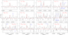 |
Fig. 1. Observed lines of l-H2C5 in TMC-1 in the 31.0–50.4 GHz range. The abscissa corresponds to the rest frequency assuming a local standard of rest velocity of 5.83 km s−1. The ordinate is antenna temperature in millikelvins. Curves shown in red are the computed synthetic spectra. The label U corresponds to features above 4σ. Frequencies and line parameters are given in Table 2. |
New derived rotational parameters (in megahertz) for l-H2C5.
As l-H2C5 has C2v symmetry, it is necessary to discern between ortho-l-H2C5 and para-l-H2C5. The ortho levels are described by Ka odd, while the para levels are described by Ka even. The nuclear spin weights are three and one for ortho-l-H2C5 and para-l-H2C5, respectively. The JKa, Kc = 11, 1 is the lowest ortho energy state located 13.4 K above the para ground level, JKa, Kc = 00, 0. Hence, from the eleven observed lines, eight of them correspond to ortho-l-H2C5 and the remaining three correspond to para-l-H2C5. An analysis of the line intensities through a line model fitting procedure by Cernicharo et al. (2021a) provides a rotational temperature of ∼10 K and column densities of N(ortho-l-H2C5) = (1.3 ± 0.3)×1010 cm−1 and N(para-l-H2C5) = (5.0 ± 2.0)×109 cm−1. The ortho/para ratio was calculated to be 2.6 ± 1.5. We have assumed a linewidth of 0.6 km s−1 and a source of uniform brightness temperature with a diameter of 80″ (Fossé et al. 2001). Figure 1 shows the computed synthetic spectrum in red.
3.2. Column densities for l-H2C3, l-H2C4, and l-H2C6 in TMC-1
The carbene l-H2C3 is the smallest cumulene species studied in this work. The laboratory spectroscopic data used to predict the l-H2C3 spectrum were reported by Vrtilek et al. (1990). The electric dipole moment calculated for this molecule is 4.1 D (Defrees & McLean 1986). As for l-H2C5, l-H2C3 has C2v symmetry and, thus, it is necessary to discern between ortho and para l-H2C3. In the same manner than for l-H2C5, the ortho levels are described by Ka odd while the para levels are described by Ka even, with a 3/1 ratio for ortho/para. Only three rotational transitions for l-H2C3 lie within the 31.0–50.4 GHz frequency range. One transition, 20, 2–10, 1, corresponds to para-l-H2C3 and the other two, 21, 2–11, 1 and 21, 1–11, 0, are ortho-l-H2C3 transitions. The lines are shown in Fig. 2, while the line parameters are collected in Table 2. The position of the lines is consistent with the calculated frequencies and the systemic velocity of the source, VLSR = 5.83 km s−1 (Cernicharo et al. 2020). We assumed Tr = 10 K and the column densities N(ortho-l-H2C3) = (1.5 ± 0.5)×1012 cm−1 and N(para-l-H2C3) = (4.0 ± 1.2)×1011 cm−1. The ortho/para ratio was calculated to be 3.8 ± 1.1. Collisional rates are available for the system l-H2C3/He (Khalifa et al. 2019). Adopting a volume density for TMC-1 of 4 × 104 cm−3 (Cernicharo & Guélin 1987; Fossé et al. 2001), we derived an excitation temperature for the two ortho transitions of ∼9 K, and of ∼8.5 K for the para transition. Hence, the adopted rotational temperature seems well adapted to the excitation conditions of this molecule.
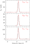 |
Fig. 2. Observed lines of l-H2C3 in TMC-1 in the 31.0–50.4 GHz range. Curves shown in red are the computed synthetic spectra. Frequencies and line parameters are given in Table 2. |
Line parameters for the lines of l-H2C3, l-H2C4, l-H2C5, and l-H2C6 observed in TMC-1.
The next member of the l-H2Cn family is l-H2C4. The rotational spectrum for this cumulene was observed by Killian et al. (1990) and Travers et al. (1996). From ab initio calculations for the dipole moment of l-H2C4 was estimated to be 4.1 D (Oswald & Botschwina 1995), similar to the smaller cumulene carbene l-H2C3. The lines for ortho- and para-l-H2C4 are clearly detected in our TMC-1 survey, as can be seen in Fig. 3. However, it should be noted that there are small discrepancies (of about 30 kHz for the para species) between the observed and predicted frequencies from CDMS. We observed a total of six rotational transitions with Jup = 4 and 5 and Ka = 0 and 1. Four of them pertain to ortho-l-H2C4 and two pertain to para-l-H2C4. All the line parameters are given in Table 2. From the observed integrated line intensities, we obtained a Tr = 10 K and column densities for the ortho and para species of N(ortho-l-H2C4) = (2.5 ± 0.8)×1012 cm−1 and N(para-l-H2C4) = (8.0 ± 2.3)×1011 cm−1. The ortho/para ratio for l-H2C4 is 3.1 ± 0.9.
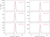 |
Fig. 3. Observed lines of l-H2C4 in TMC-1 in the 31.0–50.4 GHz range. Curves shown in red and green are the computed synthetic spectra using the observed frequencies and the CDMS predictions, respectively. Frequencies and line parameters are given in Table 2. |
To date, l-H2C6 is the larger cumulene carbene observed in space. Its dipole moment is calculated (Maluendes & McLean 1992) to be larger than those for the smaller cumulenes, with a value of 6.2 D. The rotational spectrum was investigated by McCarthy et al. (1997) and the derived spectroscopic parameters are used to predict its transition frequencies. Due to its larger molecular size, many rotational transition for l-H2C6 can be observed in the 31.0–50.4 GHz frequency range. As for all the other cumulene carbenes, and due to its symmetry, it is necessary to discern between ortho- and para-l-H2C6. Hence, we observed a total of twenty-one transitions for l-H2C6, fourteen for ortho- and seven for para-l-H2C6 (see Fig. 4). Line parameters are collected in Table 2. From the observed integrated line intensities, we derived a Tr = 10 K and the column densities N(ortho-l-H2C6) = (6.0 ± 1.8)×1010 cm−1 and N(para-l-H2C3) = (2.0 ± 0.6)×1010 cm−1. The ortho/para ratio was calculated to be 3.0 ± 0.9.
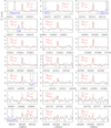 |
Fig. 4. Observed lines of l-H2C6 in TMC-1 in the 31.0–50.4 GHz range. Curves shown in red are the computed synthetic spectra. Frequencies and line parameters are given in Table 2. |
From our observations, we obtain the following relative abundances for l-H2C3/l-H2C4/l-H2C5/l-H2C6 in TMC-1, 344/561/1/4.4. l-H2C4 is the most abundant cumulene carbene in TMC-1, followed by l-H2C3. The larger species, l-H2C5 and l-H2C6, are much less abundant compared to the shorter cumulene chain, with l-H2C6 being 4.4 times more abundant than the odd member l-H2C5. It is worth noting that, within the uncertainties, the four cumelenes studied in this work have an ortho/para abundance ratio of 3. Hence, no significant ortho to para conversion can be noticed for these molecules.
3.3. Chemistry of cumulene carbenes
In order to understand how cumulene carbenes l-H2Cn can be formed in TMC-1, we carried out gas-phase chemical modelling calculations. We adopted typical conditions of cold dark clouds, that is, a volume density of H nuclei of 2 × 104 cm−3, a gas kinetic temperature of 10 K, a visual extinction of 30 mag, a cosmic-ray ionisation rate of H2 of 1.3 × 10⁻¹⁷ s−1, and the so-called set of low-metal elemental abundances (e.g., Agúndez & Wakelam 2013). We used the chemical network RATE12 from the UMIST database (McElroy et al. 2013), updated with results from Lin et al. (2013) and with the subset of gas-phase chemical reactions revised by Loison et al. (2017) in their study of the chemistry of C3H and C3H2 isomers.
Among the family of carbenes l-H2Cn, the one for which the chemistry is better constrained is by far the smallest member l-H2C3, which has been discussed in detail by Loison et al. (2017). This species is mainly formed upon dissociative recombination with electrons of the linear and cyclic isomers of C3 , which in turn are formed through the radiative association of C3H+ and H2. If we focus on the so-called early time, a few 105 yr, where gas-phase chemical models of cold dark clouds reproduce better TMC-1 observations (e.g., Agúndez & Wakelam 2013), the calculated abundance is about one order of magnitude below the observed value (see Fig. 5), but the calculated cyclic-to-linear abundance ratio agrees very well with the observed value of 31 (Cernicharo et al. 2021a; this work). For members of the series l-H2Cn with n > 3, information on the chemistry of the different possible isomers is poorly known and thus chemical networks, such as UMIST RATE12, do not distinguish between them. The calculated abundances of C4H2 and C6H2 agree within a factor of 2 and 3 with the observed abundances of l-H2C4 and l-H2C6, respectively (see Fig. 5). Although one must keep in mind that observations only refer to the cumulene, while the model also includes other isomers, in particular the more stable non-polar species HCnH. If the isomer HCnH is significantly more abundant than H2Cn for n = 4, 6 in TMC-1, then the abundances calculated by the chemical model for C4H2 and C6H2 would be too low. In the case of C5H2, the calculated peak abundance is about 30 times lower than the observed abundance of l-H2C5 (see Fig. 5), although this may not be a problem if the more stable isomer HC5H is substantially more abundant than the carbene l-H2C5.
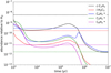 |
Fig. 5. Calculated fractional abundances of various hydrocarbons as a function of time. The asterisk in the legend means that the chemical model does not distinguish between different isomers. The abundances observed in TMC-1 for c-C3H2 (Cernicharo et al. 2021a) and l-H2Cn with n = 3−6 (this work) are indicated by dashed horizontal lines. |
For l-H2Cn with n > 3, the chemical route analogous to that forming l-H2C3 has variable degrees of efficiency. For example, formation of C4 is relatively efficient thanks to the radiative association between C4
 and H (McEwan et al. 1999). For n = 5, the route does not work because C5H+ does not react with H2 (McElvany & Dunlap 1987; Bohme & Wlodek 1990), while formation of C6
 is uncertain due to the unknown reactivity of C6
 with H2 (Anicich 2003). Further studies of reactions involving hydrocarbon ions, in particular regarding isomer differentiation, are highly desirable. According to the chemical model, reactions of CnH− anions with H atoms are a major route to CnH2 molecules, such as C4H2, C5H2, and C6H2. These reactions have been studied in the laboratory for anions CnH− with n = 2, 4, 6, and 7 and have been found to be rapid and to yield CnH2 as a main product (Barckholtz et al. 2001). The reaction with n = 5, although not studied, is likely to behave similarly. It is however unknown whether the carbene isomer H2Cn or the more stable HCnH is preferentially formed. It would be very helpful to investigate this particular point.
Other formation routes, apart from Cn and CnH− + H, can be provided by neutral-neutral reactions. For example, the chemical model points to the reaction between atomic C and the propargyl radical (CH2CCH), which was recently detected in TMC-1 (Agúndez et al. 2021), as a source of C4H2 isomers. This reaction is assumed to be fast by Loison et al. (2017), but calculations of the rate coefficient and product distribution at low temperatures are needed. Similarly, the reaction C + C4H3 is assumed to proceed quickly by Smith et al. (2004) and provides an important route to C5H2 isomers, but more detailed studies on this reaction are necessary. Finally, we note that the cyclic C5H2 isomer c-C3HCCH recently detected by Cernicharo et al. (2021a) is most likely formed through the reaction between CCH and c-C3H2.
Acknowledgments
This research has been funded by ERC through grant ERC-2013-Syg-610256-NANOCOSMOS. Authors also thank Ministerio de Ciencia e Innovación for funding support through projects AYA2016-75066-C2-1-P, PID2019-106235GB-I00 and PID2019-107115GB-C21/AEI/10.13039/501100011033. MA thanks Ministerio de Ciencia e Innovación for grant RyC-2014-16277.
References
- Agúndez, M., & Wakelam, V. 2013, Chem. Rev., 113, 8710 [Google Scholar]
- Agúndez, M., Cabezas, C., Tercero, B., et al. 2021, A&A, 647, L10 [EDP Sciences] [Google Scholar]
- Anicich, V. G. 2003, JPL Publication 03–19 [Google Scholar]
- Araki, M., Takano, S., Sakai, N., et al. 2017, ApJ, 847, 51 [NASA ADS] [CrossRef] [Google Scholar]
- Barckholtz, C., Snow, T. P., & Bierbaum, V. M. 2001, ApJ, 547, L171 [NASA ADS] [CrossRef] [Google Scholar]
- Bohme, D. K., & Wlodek, S. 1990, Int. J. Mass Spectrom. Ion Proc., 102, 133 [CrossRef] [Google Scholar]
- Cernicharo, J. 1985, Internal IRAM Report (Granada: IRAM) [Google Scholar]
- Cernicharo, J. 2012, in European Conference on Laboratory Astrophysics, eds. C. Stehlé, C. Joblin, & L. d’Hendecourt, EAS Publ. Ser., 58, 251 [Google Scholar]
- Cernicharo, J., & Guélin, M. 1987, A&A, 176, 299 [Google Scholar]
- Cernicharo, J., Gottlieb, C. A., Guélin, M., et al. 1991a, ApJ, 368, L39 [NASA ADS] [CrossRef] [Google Scholar]
- Cernicharo, J., Gottlieb, C. A., Guélin, M., et al. 1991b, ApJ, 368, L43 [NASA ADS] [CrossRef] [Google Scholar]
- Cernicharo, J., Heras, A. M., Tielens, A. G. G. M., et al. 2001, ApJ, 546, L123 [NASA ADS] [CrossRef] [Google Scholar]
- Cernicharo, J., Guélin, M., Agúndez, M., et al. 2018, A&A, 618, A4 [NASA ADS] [CrossRef] [EDP Sciences] [Google Scholar]
- Cernicharo, J., Marcelino, N., Agúndez, M., et al. 2020, A&A, 642, L8 [NASA ADS] [CrossRef] [EDP Sciences] [Google Scholar]
- Cernicharo, J., Agúndez, M., Cabezas, C., et al. 2021a, A&A, 649, L5 [CrossRef] [EDP Sciences] [Google Scholar]
- Cernicharo, J., Cabezas, C., Endo, Y., et al. 2021b, A&A, 646, L3 [EDP Sciences] [Google Scholar]
- Cernicharo, J., Cabezas, C., Bailleux, S., et al. 2021c, A&A, 646, L7 [NASA ADS] [CrossRef] [EDP Sciences] [Google Scholar]
- Defrees, D. J., & McLean, A. D. 1986, ApJ, 308, 31 [NASA ADS] [CrossRef] [Google Scholar]
- Fossé, D., Cernicharo, J., Gerin, M., & Cox, P. 2001, ApJ, 552, 168 [Google Scholar]
- Gottlieb, C. A., McCarthy, M. C., Gordon, V. D., et al. 1998, ApJ, 509, L141 [NASA ADS] [CrossRef] [Google Scholar]
- Guélin, M., Müller, S., & Cernicharo, J. 2000, A&A, 363, L9 [Google Scholar]
- Herbst, E. 1978, ApJ, 222, 508 [NASA ADS] [CrossRef] [Google Scholar]
- Kawaguchi, K., Kaifu, N., Ohishi, M., et al. 1991, PASJ, 43, 607 [NASA ADS] [Google Scholar]
- Khalifa, M. B., Sahnoun, E., Wiesenfeld, L., et al. 2019, Phys. Chem. Chem. Phys., 21, 1443 [CrossRef] [Google Scholar]
- Killian, T. C., Vrtilek, J. M., Gottlieb, C. A., et al. 1990, ApJ, 365, L89 [CrossRef] [Google Scholar]
- Langer, W. D., Velusamy, T., Kuiper, T. B. H., et al. 1997, ApJ, 480, L63 [NASA ADS] [CrossRef] [Google Scholar]
- Lin, Z., Talbi, D., Roueff, E., et al. 2013, ApJ, 765, 80 [NASA ADS] [CrossRef] [Google Scholar]
- Loison, J.-C., Agúndez, M., Wakelam, V., et al. 2017, MNRAS, 470, 4075 [NASA ADS] [CrossRef] [Google Scholar]
- Maluendes, S. A., & McLean, A. D. 1992, Chem. Phys. Lett., 200, 511 [NASA ADS] [CrossRef] [Google Scholar]
- McCarthy, M. C., Travers, M. J., Kovács, A., et al. 1997, Science, 275, 518 [NASA ADS] [CrossRef] [Google Scholar]
- McElroy, D., Walsh, C., Markwick, A. J., et al. 2013, A&A, 550, A36 [NASA ADS] [CrossRef] [EDP Sciences] [Google Scholar]
- McElvany, S. W., Dunlap, B. I., & OḰeefe, A., 1987, J. Chem. Phys., 86, 715 [CrossRef] [Google Scholar]
- McEwan, M. J., Scott, G. B. I., Adams, N. G., et al. 1999, ApJ, 513, 287 [NASA ADS] [CrossRef] [Google Scholar]
- Müller, H. S. P., Schlöder, F., Stutzki, J., & Winnewisser, G. 2005, J. Mol. Struct., 742, 215 [Google Scholar]
- Oswald, M., & Botschwina, P. 1995, J. Mol. Spectrosc., 169, 181 [NASA ADS] [CrossRef] [Google Scholar]
- Pardo, J. R., Cernicharo, J., & Serabyn, E. 2001, IEEE Trans. Antennas Propag., 49, 12 [Google Scholar]
- Sattelmeyer, K. W., & Stanton, J. F. 2000, J. Am. Chem. Soc., 122, 8220 [CrossRef] [Google Scholar]
- Seburg, R. A., McMahon, R. J., Stanton, J. F., & Gauss, J. 1997, J. Am. Chem. Soc., 119, 10838 [Google Scholar]
- Smith, I. W. M., Herbst, E., & Chang, Q. 2004, MNRAS, 350, 323 [NASA ADS] [CrossRef] [Google Scholar]
- Tercero, F., López-Pérez, J. A., Gallego, F., et al. 2021, A&A, 645, A37 [EDP Sciences] [Google Scholar]
- Thaddeus, P., Vrtilek, J. M., & Gottlieb, C. A. 1985, ApJ, 299, L63 [NASA ADS] [CrossRef] [Google Scholar]
- Travers, M. J., Chen, W., Novick, S. E., et al. 1996, J. Mol. Spectrosc., 180, 75 [CrossRef] [Google Scholar]
- Travers, M. J., McCarthy, M. C., Gottlieb, C. A., & Thaddeus, P. 1997, ApJ, 483, L135 [NASA ADS] [CrossRef] [Google Scholar]
- Vrtilek, J. M., Gottlieb, C. A., Gottlieb, E. W., et al. 1990, ApJ, 364, L53 [NASA ADS] [CrossRef] [Google Scholar]
All Tables
Line parameters for the lines of l-H2C3, l-H2C4, l-H2C5, and l-H2C6 observed in TMC-1.
All Figures
|
Fig. 1. Observed lines of l-H2C5 in TMC-1 in the 31.0–50.4 GHz range. The abscissa corresponds to the rest frequency assuming a local standard of rest velocity of 5.83 km s−1. The ordinate is antenna temperature in millikelvins. Curves shown in red are the computed synthetic spectra. The label U corresponds to features above 4σ. Frequencies and line parameters are given in Table 2. |
| In the text | |
|
Fig. 2. Observed lines of l-H2C3 in TMC-1 in the 31.0–50.4 GHz range. Curves shown in red are the computed synthetic spectra. Frequencies and line parameters are given in Table 2. |
| In the text | |
|
Fig. 3. Observed lines of l-H2C4 in TMC-1 in the 31.0–50.4 GHz range. Curves shown in red and green are the computed synthetic spectra using the observed frequencies and the CDMS predictions, respectively. Frequencies and line parameters are given in Table 2. |
| In the text | |
|
Fig. 4. Observed lines of l-H2C6 in TMC-1 in the 31.0–50.4 GHz range. Curves shown in red are the computed synthetic spectra. Frequencies and line parameters are given in Table 2. |
| In the text | |
|
Fig. 5. Calculated fractional abundances of various hydrocarbons as a function of time. The asterisk in the legend means that the chemical model does not distinguish between different isomers. The abundances observed in TMC-1 for c-C3H2 (Cernicharo et al. 2021a) and l-H2Cn with n = 3−6 (this work) are indicated by dashed horizontal lines. |
| In the text | |
Current usage metrics show cumulative count of Article Views (full-text article views including HTML views, PDF and ePub downloads, according to the available data) and Abstracts Views on Vision4Press platform.
Data correspond to usage on the plateform after 2015. The current usage metrics is available 48-96 hours after online publication and is updated daily on week days.
Initial download of the metrics may take a while.