| Issue |
A&A
Volume 653, September 2021
|
|
|---|---|---|
| Article Number | A7 | |
| Number of page(s) | 22 | |
| Section | Extragalactic astronomy | |
| DOI | https://doi.org/10.1051/0004-6361/202140583 | |
| Published online | 31 August 2021 | |
Possible evidence for a supermassive binary black hole in 3C454.3
1
National Astronomical Observatories, Chinese Academy of Sciences, Beijing 100012, PR China
e-mail: rqsj@bao.ac.cn
2
Max-Planck Institut für Radioastronomie, Bonn, Germany
Received:
16
February
2021
Accepted:
15
May
2021
Context. The kinematic behaviors of thirteen superluminal components observed at 43 GHz in blazar 3C454.3 are investigated and model-fitted in terms of the precessing jet-nozzle scenario previously proposed.
Aims. In order to search for the possible precession of jet-nozzle and periodic ejection of superluminal components in 3C454.3, the thirteen components are divided into the following two groups: group-A and group-B. Group-A consists of six components (B4, B5, K2, K3, K09, and K14) and group-B consists of seven components (B1, B2, B3, B6, K1, K10, and K16).
Methods. For each component of group-A and group-B, the observed kinematic features (trajectory, core separation, coordinates, and apparent velocity versus time) were model-fitted in terms of our precessing jet-nozzle scenario, and its kinematic parameters (bulk Lorentz factor, viewing angle, apparent velocity, and Doppler factor versus time) were derived and compared with the observations.
Results. It is found that the superluminal components of group-A and group-B may be regarded to be produced by a double-jet system, consisting of jet-A and jet-B which ejects the components of group-A and group-B, respectively. Both jets are likely precessing with the same period of ∼10.5 yr (5.6 yr in the source frame) with modeled time coverages of ∼2 and ∼1.5 periods, respectively. The motion of these components in the inner-jet regions (core separation ≲0.3–0.5 mas) is explained to follow a precessing common trajectory respective for jet-A and jet-B. The recurrence of the curved trajectory for the pair of knots B6 and K10 exhibits a significant clue as to periodicity.
Conclusions. The analysis and explanation of the entire kinematics of the thirteen superluminal components observed in 3C454.3 in terms of our precessing jet-nozzle scenario might possibly imply that blazar 3C454.3 hosts a supermassive binary black hole, which creates two precessing relativistic jets pointing closely toward us with small angles.
Key words: radio continuum: galaxies / galaxies: jets / galaxies: kinematics and dynamics / quasars: individual: blazar 3C454.3
© ESO 2021
1. Introduction
The blazar 3C454.3 (redshift z = 0.859) is one of the most prominent and well-studied blazars. It is a flat-spectrum radio quasar and an optically violent variable with large and rapid polarized outbursts in radio and optical bands. It radiates across the entire electromagnetic spectrum from radio and millimeter through IR-optical-UV and X-ray to high-energy γ-rays. Long-term and short-term monitoring observations reveal various variability timescales from hours, days, and even to years.
In recent years, coordinated observations in radio, IR-optical-UV, X-ray, and γ-rays combined with very long base-line interferometry (VLBI) observations have provided important information, clarifying some physical issues, for example the interpretation of its spectral energy distributions at flaring and quiescent states and the relative location of γ-ray and optical emitting regions in the jet.
Since 2005, the blazar 3C454.3 has shown remarkable flaring activity at all frequencies from radio to γ-rays. In optical and X-ray bands in May 2005, 3C454.3 showed an extremely bright state from the near-infrared (NIR) to the hard X-rays, with the optical flare reaching an optical magnitude mR(R-band) = 12 mag (an unprecedented brightness level), which was followed by a millimeter outburst and flux increase at high radio frequencies (Raiteri et al. 2007; Villata et al. 2006; Fuhrmann et al. 2006). However, in early 2006, a major millimeter flare was observed, which is associated with a minor optical flare.
During the period 2007–2010, 3C454.3 exhibited extremely strong and exceptional γ-ray (> 100 MeV) activities and, in particular, it was observed to be the brightest γ-ray source in the sky on 2009 December 2-3 and 2010 November 20 (a factor of ∼2 and ∼6 brighter than the Vela pulsar, respectively; Donnarumma et al. 2009; Vercellone et al. 2009, 2010, 2011 and references therein). Both γ-ray flares were associated with ejections of radio knots (K09 and K10) observed by VLBI observations (Jorstad et al. 2013; see below)
Multiwavelength monitoring campaigns have been carried out during periods of γ-ray flares, obtaining a large amount of data from radio through optical and X-ray to high-energy γ-rays. A large number of observational and theoretical works have been carried out, emphasizing the following: the correlation (and time delays) between light curves at different energy bands (especially between γ-rays and radiations at radio and optical bands), spectral energy distribution (SED), radiation mechanisms for γ-rays, extremely fast γ-ray variability on < 10hr timescales, the relation between γ-ray outbursts and the ejection of superluminal components on VLBI scales, etc. These studies greatly deepen our understanding of the generic properties of γ-ray blazars and clarify some theoretical issues (e.g., Abdo et al. 2009, 2010, 2011; Ghisellini et al. 2007; Sikora et al. 2008, 2009; Marscher 2013; Foschini et al. 2011; Tosti 2007; Bonnoli et al. 2011; Bonning et al. 2009, 2012; Donnarumma et al. 2009; Giommi et al. 2006; Finke & Dermer 2010; Pacciani et al. 2010; Pian et al. 2006; Ogle et al. 2011; Jorstad et al. 2017, 2013, 2010; Wehrle et al. 2012; Raiteri et al. 2011, 2008a,b, 2007; Striani et al. 2010; Villata et al. 2006, 2007, 2009; Vercellone 2012a,b, Vercellone et al. 2009, 2010, 2011, 2008, 2009).
As an extremely variable flat-spectrum radio quasar, 3C454.3 is one of the most prominent superluminal sources and its superluminal components were firstly detected from the 1981–1986 VLBI observations at centimeter wavelengths (Pauliny-Toth et al. 1987; Pauliny-Toth 1998). They detected some peculiar features on parsec scales: (1) superluminal brightening of the core; (2) the coexistence of a stationary component and superluminally moving components; (3) apparent acceleration of knots; and (4) extremely apparent curvature of the trajectory. These features could be understood now in terms of the formation of stationary shocks or apparently stationary patterns in a curved jet (e.g., Daly & Marscher 1988; Gomez et al. 1997; Meier & Nakamura 2006). Britzen et al. (2013) investigated its VLBI structure and evolution at 15 GHz during a ∼16 yr period (1995.6–2011.5), finding a superluminally expanding ring structure. They also suggest that the ejection position angle swing revealed by the superluminal components could be explained in terms of periodic jet precessing and nutation. Qian et al. (2014) tried to explain the kinematics (trajectory, core separation, coordinates, and apparent velocity versus time) of its nine superluminal knots in terms of the precessing jet-nozzle scenario (Qian et al. 1991, 2009, 2019) and to yield their kinematic parameters (viewing angle, bulk Lorentz factor, and Doppler factor versus time).
Multifrequency monitoring campaigns conducted during the period from approximately 2000–2010 strongly revealed that the multifrequency outbursts across the entire electromagnetic spectrum (from radio-optical-X-ray to high energy γ-rays) are closely connected to the ejections of the superluminal components. In particular, the correlation between the high energy γ-ray outbursts and the ejection of superluminal components is most remarkable (e.g., Jorstad et al. 2005, 2010, 2013; Jorstad et al. 2017; Wehrle et al. 2012).
In this paper we would like to investigate the periodic or quasi-periodic behavior in the ejection of superluminal components in 3C454.3. The search for periodicity in the optical and radio light curves of 3C454.3 has been done, for example, by Su (2001) and Pyatunina et al. (2004). Kudryavtseva & Pyatunina (2008) found the presence of a period 12.4 ± 0.6 yr by means of analyzing the centimeter light curves with the discrete auto-correlation function method. Qian et al. (2007) noticed the double-bump structure in the centimeter light curves with a quasi-periodicity of ∼12.8 yr and proposed a rotating double-jet model to fit the centimeter light curves and the possible presence of a black hole binary. This proposal seems instructive because we show that the kinematic behavior of the superluminal components could be explained in terms of a double precessing jet-nozzle system as described below.
In fact, several years ago we speculated that 3C454.3 might possibly host a double-jet system created by a supermassive binary black hole in its nucleus because we had noticed the following observational facts.
– We noticed the double-bump structure in its centimeter light curves with a pair of outbursts (one strong and one weaker) quasi-regularly separated in time and a quasi-periodicity ∼12.8 yr, which had exhibited for three periods (1965–2005; Kudryavtseva & Pyatunina 2008; Qian et al. 2007).
– As pointed out by Jorstad et al. (2005), the moving components in 3C454.3 should be separated into two groups because rapid swings of the ejection position angle were observed. For example, the difference between the ejection position angles of knots B6 and B4 reaches ∼70°, while the difference between their ejection times is only ∼1.5 yr. We thought that this rapid swing of the ejection position angle is difficult to be explained in a single-jet scenario1.
– Later on, the VLBI observations performed by Jorstad et al. (2013) allowed for them to find that another pair of superluminal knots, K09 and K10, have a behavior similar to that of the pair of knots B4 and B6. The difference between their ejection times is ∼1.1 yr, while the difference between their ejection position angles (measured by their first data points) reaches ∼60°. This pair also showed a rapid ejection position angle swing.
– In particular, knot K10 has a strongly curved path within a core separation ∼0.1 mas, which is very similar to that of knot B6, possibly indicating that both knots, B6 and K10, could be ascribed to a jet, while B4 and K09 could be ascribed to another jet. We thought that the recurrence of a curved trajectory for knots K10 and B6 may be a significant indication for periodicity. We also noticed that the difference between the ejection times of knots K10 and B6 and that for K09 and B4 are similar, being ∼11 yr, which is only a bit shorter than that derived from the analysis of the radio light curves of the source (Qian et al. 2007). Therefore 3C454.3 could have a period ∼11–12 yr of its precessing jet nozzle, yielding the periodicity in the ejection of superluminal knots.
However, at that time, we were not able to find a specific (or concrete) model to disentangle the complex kinematic behavior originating from a double jet system assumed for 3C454.3. Fortunately, the data recently published on the knots K14 and K16 (Liodakis et al. 2020; Weaver et al. 2019) are very useful for testing the application of our double precessing jet scenario assumed for 3C454.3.
In the following, we further analyze and model-fit the kinematics of the 13 superluminal knots of 3C454.3 in terms of our precessing jet-nozzle scenario. We also discuss the suggestion of a black hole binary system, producing the two relativistic jets.
In this paper we adopt the concordant cosmological model (Λ cold dark matter (ΛCDM) model) with Ωm = 0.3, ΩΛ = 0.7, and a Hubble constant of H0 = 70 km s−1 Mpc−1 (Spergel et al. 2003). Thus for 3C454.3, z = 0.859, its luminosity distance is Dl = 5.483 Gpc (Hogg 1999; Ue-Li 1999), and the angular diameter distance is Da = 1.586 Gpc. The angular scale 1 mas = 7.69 pc and proper motion of 1 mas yr−1 are equivalent to an apparent velocity of 46.58c.
We made use of the observation data collected from the following works: Jorstad et al. (2001, 2005, 2010), and Jorstad et al. (2013) for knots B1, B2, B3, B4, B5, B6, K1, K2, K3, K09, and K10; Liodakis et al. (2020) for knot K14; and Weaver et al. (2019) for knot K16. We made model-fits to the kinematic behaviors of the knots and present the obtained results in our figures. Generally, we did not mark the observational errors in the data points, but kept the typical observational errors in coordinates ∼0.02–0.1 mas in mind. We propose new criteria for judging the quality of model-fitting in a knot’s trajectory and a period of jet-nozzle precession.
2. Geometry and formalism
In order to investigate the kinematic behavior and distribution of the trajectory of superluminal components in blazar 3C454.3 on parsec scales in terms of our precessing jet-nozzle scenario, we used a special geometry described as follows (also see Qian et al. 2017, 2019, 2009; Qian et al. 1991).
First, generally, we assume that the superluminal components move along helical trajectories around the curved jet axis (i.e., axis of the helix), as shown in Fig. 1.
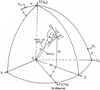 |
Fig. 1. Geometry of the precession helical trajectory model. Superluminal knots move along a helical trajectory around the jet axis defined by the function x0(z0) in the plane (X, Z), having an amplitude A(s0) and phase ϕ(s0) defined in the coordinate system (x′, y′, z′). Through transformation among the coordinate systems, the apparent trajectory and the kinematic parameters (bulk Lorentz factor, Doppler factor, apparent velocity, and viewing angle) of a knot can be derived from its spatial trajectory and spatial kinematics by using the formulas given in Sect. 2. |
Second, we used the coordinate system (Xn, Yn, Zn) to define the plane of the sky (Xn, Zn) and the direction of the observer (Yn), with the Xn-axis pointing toward the negative right ascension and the Zn-axis pointing toward the north pole.
Third, we introduced the coordinate system (X, Y, Z) and located the curved jet axis in the plane (X, Z), where ϵ represents the angle between the Z-axis and Yn-axis and ψ is the angle between the X-axis and Xn-axis. Thus parameters ϵ and ψ were used to define the plane where the jet axis is located.
Fourth, we further introduced the coordinate system (x′, y′, z′) along the jet axis, and we then could use parameters A(s0) (amplitude) and ϕ(s0) (phase) to define the helical trajectory of a knot, where s0 represents the arclength along the axis of helix (or jet axis). The z′-axis is along the tangent of the jet axis.
Fifth, in general, we assume that the jet axis can be defined by a function x0(z0) in the plane (X, Z). We assume the following form for this function:
where
![$$ \begin{aligned} p({z_0}) = {p_1}+{p_2}\left[1+\mathrm{exp}\left(\frac{{z_t}-{z_0}}{{z_m}}\right)\right]^{-1} \end{aligned} $$](/articles/aa/full_html/2021/09/aa40583-21/aa40583-21-eq2.gif)
here ζ = 2 and p(z0) = constant represent a simple parabolic shape. We note that p1, p2, zt, and zm are constants that can be chosen to define the curved jet axis (or the axis of the helix). The arclength along the jet axis s0 is:
In our precession nozzle scenario, the amplitude (A(s0)) and helical phase (ϕ(s0)) of the helical trajectory are specifically defined for the jets (jet-A and jet-B). The initial phase ϕ0 = ϕ(t = 0) for a knot is assumed to be the precession phase of the knot. Different knots have different helical trajectories described by their initial phase ϕ0, which precesses during a precession period.
We have described how to define the spatial helical trajectory of a superluminal knot. Using the following formulas, we can calculate the apparent kinematic parameters observed by VLBI observations: trajectory Xn(Zn), coordinates Xn(t) and Zn(t), core separation rn(t), apparent velocity βa(t) and viewing angle θ(t), bulk Lorentz factor Γ(t), and Doppler factor δ(t).
The spatial helical trajectory of a knot can be described in an (X, Y, Z) system as follows:


where tanη(s0) =  . The projection of the helical trajectory on the plane of the sky (or the apparent trajectory) is represented by
where


All coordinates and the amplitude (A) were measured in units of milliarcseconds. We introduced the following functions
![$$ \begin{aligned} {\Delta }=\arctan \left[\left(\frac{\mathrm{d}X}{\mathrm{d}Z}\right)^2+\left(\frac{\mathrm{d}Y}{\mathrm{d}Z}\right)^2\right]^{-\frac{1}{2}} \end{aligned} $$](/articles/aa/full_html/2021/09/aa40583-21/aa40583-21-eq12.gif)
![$$ \begin{aligned} {{\Delta }_s}=\arccos \left[\left(\frac{\mathrm{d}X}{\mathrm{d}{s_0}}\right)^2+\left(\frac{\mathrm{d}Y}{\mathrm{d}{s_0}}\right)^2+ \left(\frac{\mathrm{d}Z}{\mathrm{d}{s_0}}\right)^2\right]^{-\frac{1}{2}} .\end{aligned} $$](/articles/aa/full_html/2021/09/aa40583-21/aa40583-21-eq14.gif)
And we could then calculate the viewing angle θ, apparent transverse velocity βa, Doppler factor δ, and the elapsed time T, at which the knot reaches distance z0, as follows:
![$$ \begin{aligned} {\theta }=\arccos [{\cos {\epsilon }}(\cos {\Delta }+ \sin {\epsilon }\tan {{\Delta }_p})] \end{aligned} $$](/articles/aa/full_html/2021/09/aa40583-21/aa40583-21-eq15.gif)
![$$ \begin{aligned} {\delta }=[{\Gamma }(1-{\beta }{\cos {\theta }})]^{-1} \end{aligned} $$](/articles/aa/full_html/2021/09/aa40583-21/aa40583-21-eq16.gif)

where Γ = ![$ [1-{\beta}^2]^{-\frac{1}{2}} $](/articles/aa/full_html/2021/09/aa40583-21/aa40583-21-eq19.gif) –bulk Lorentz factor, β = v/c, and v is the velocity of the knot.
–bulk Lorentz factor, β = v/c, and v is the velocity of the knot.
In Sects. 3 and 4, we perform model-fits to the kinematics of the superluminal knots ejected from jet-A and jet-B, respectively. The aim is to use our precessing nozzle scenario to make reasonable fits to the observed parameters of their observed kinematic behavior (including the apparent trajectory, coordinates, core separation, apparent velocity, bulk Lorentz factor, and Doppler factor) and to determine the precession period of the jet nozzles, yielding possible evidence for the existence of a supermassive black hole binary in blazar 3C454.3.
3. Model-fitting of kinematics of superluminal knots of jet-A
Investigating the kinematics of superluminal knots in blazar 3C454.3 in terms of our precessing nozzle scenario, we have found that 3C454.3 might contain two relativistic jets, which eject superluminal components, respectively. Both jet nozzles precess with a period of ∼10.5 yr in a counterclockwise direction. We made model-fits to the kinematics of superluminal components for both jets, respectively.
Knots B4, B5, K2, K3, K09, and K14 are assumed to be ejected by the nozzle of jet-A. We show that their observed trajectories can be fitted well with the precessing common trajectory at the model-predicted precession phases.
In our scenario, the jet axis is defined in the (X, Y)-plane by parameters (ϵ, ψ) and formulas (1) and (2) in Sect. 2. Here for jet-A we assume2 that ϵ = 0.0126 rad (0.72°), ψ = −0.1 rad (−5.73°), and p1 = p2 = 0. Thus the Z-axis is considered to be the jet axis.
The amplitude of the common helical trajectory is assumed to be A = A0sin(πz0/Z1), with A0 = 0.727 mas and Z1 = 240 mas. The helical phase is assumed to be ϕ = constant ≡ precession phase ϕ0 = ϕ(t0) (t0 is the ejection time of a knot).
The parameters given above define the pattern of the spatial helical trajectory for jet-A, which precesses to produce the trajectory of individual knots at their corresponding precession phases. The precession phase of a knot is related to its ejection time as follows:
where T0 = 10.5 yr is the precession period of the jet-A nozzle.
When the parameters of the precessing nozzle scenario for jet-A are given as described above, we can then perform model-fitting of the observed kinematic behavior for each knot of jet-A and derive its bulk Lorentz factor and Doppler factor.
It is noteworthy that the values selected for the model parameters and the associated functions are not statistical samples nor unique. They are a specific and physically meaningful set of working ingredients, which have been obtained through trial and error over the past years, and can be applied to analyze the kinematics of superluminal knots in blazar 3C454.3 on VLBI scales. Based on our precessing nozzle scenario, possible evidence for double precessing relativistic jets and a binary black hole in 3C454.3 are tentatively discussed.
It is found that jet-A thus has a very small cone angle of ∼1.38° in space, but its projection in the plane of sky has a cone angle of ∼60° (at a core separation of ∼0.2 mas)3 with its jet axis at a position angle of ∼−84.3°. Most of the superluminal knots follow the precessing common trajectory defined above at different core separations. The modeled precessing common trajectory distribution for jet-A is shown in Fig. 2 (upper panel) and the observed trajectories of knots B5, K09, and K14 are also shown for comparison.
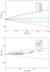 |
Fig. 2. Jet-A: Modeled precessing common trajectory distribution (upper panel) and the observed trajectories of knots B5, K09, and K14 for comparison (lower panel). |
3.1. Model-fitting of the kinematics of knot B4
The model-fitting results for the kinematics of knot B4 are shown in Fig. 3. In the model fitting, we assumed its precession phase ϕ0 = 4.58 rad and corresponding ejection time t0 = 1998.24, which is consistent with the ejection time 1998.36 ± 0.07 derived by Jorstad et al. (2005).
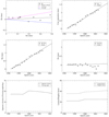 |
Fig. 3. Model fitting results for knot B4. |
It can be seen that its entire kinematics (trajectory, core separation, and coordinates versus time) are well fitted within Xn ∼ 0.9 mas. The kinematic quantities (apparent velocity, viewing angle, Lorentz factor, and Doppler factor) were derived.
In order to demonstrate the validity of model-fitting results, two modeled trajectories (in magenta and blue) defined by precession phases of 4.58 ± 0.31 rad (0.31 rad corresponding to 5% of the precession period, equivalent to 0.53 yr) are also shown in Fig. 3 (in the top left panel). We recognize that the model-fitting with the precessing common trajectory is effective if the data points obtained by VLBI observations are well within the region limited by the two lines. It can be seen that for knot B4, most of the data points are located within this region, although they are quite divergent4.
In order to explain the observed core separation rn(t), coordinates Xn(t) and Zn(t), and apparent velocity βa, changes in its bulk Lorentz factor Γ are assumed: for Z ≤ 20 mas, Γ = 22; for Z = 20−30 mas, Γ = 22 + 2.7(Z − 20)/(30−20)5; and for Z > 30 mas, Γ = 24.7. During the period from 1998.4–2000.6, the bulk Lorentz factor Γ, the Doppler factor δ, the apparent velocity βa, and the viewing angle θ vary over the following respective ranges: [22.0 → 24.7], [35.6 → 39.2], [17.3 → 19.9]c, and [1.26 → 1.18](deg.). Jorstad et al. derived those parameters to be as follows: Γ = 20.0, δ = 13.9, βa = 19.0 ± 1.1c, and θ = 3.9°. Obviously, our modeled apparent velocity is consistent with the observed value, but the values derived for δ and θ by Jorstad et al. (2005) are largely different from ours6. Therefore, the observed kinematic behavior of knot B4 can be explained well in terms of our precessing nozzle scenario with a precession period 10.5 yr within core separation ≲0.9 mas (i.e., before ∼2000.60), equivalent to a spatial distance of Zc, m ∼ 41.7 mas (or Zc, p ∼ 321 pc) from the radio core.
3.2. Model fitting of kinematics of knot B5
The model fitting results of the kinematics of knot B5 are shown in Fig. 14. Its precession phase and ejection time are modeled as ϕ0 = 4.69 rad and t0 = 1998.42, compared with 1999.04 ± 0.44 given by Jorstad et al. (2005).
Only five data points were available for its trajectory, but all are exactly on the modeled precessing common trajectory. This is good evidence for our precessing nozzle scenario for jet-A being very successful. Its common trajectory was observed to extend to a core separation of rn ∼ 0.3 mas, corresponding to a spatial distance of Zc, m ∼ 27.3 mas (or Zc, p ∼ 210 pc) from the core.
Its motion is accelerated. The bulk Lorentz factor is modeled as follows: for Z ≤ 3 mas, Γ = 9.5; for Z = 3−16 mas, Γ = 9.5 + 20.5(Z − 3)/(16−3); and for Z > 16 mas, Γ = 30. During the 1999.4–2000.4 period, its Lorentz factor Γ, Doppler factor δ, apparent velocity βa, and viewing angle θ approximately vary over the ranges of [11.0 → 30.0], [20.5 → 41.9], [5.0 → 27.5]c, and [1.25 → 1.27](deg.), respectively. Thus we can see that the observed kinematic behavior of knot B5 can be explained well in terms of the precessing jet-nozzle model for jet-A.
3.3. Model fitting of kinematics of knot K2
Knots K2 and K3 may be a pair of superluminal ejections and they are connected with the γ-ray outburst on 2007 July 24–30 (Vercellone et al. 2010). For the model fitting of the kinematics of knot K2, we considered the following two cases: t0 = 2007.49 and t0 = 2007.24.
3.3.1. Case 1: t0 = 2007.49
We adopted its ejection time t0 = 2007.49 as suggested by Jorstad et al. (2010), corresponding to precession phase ϕ0(rad) = 3.83 + 2π. The model-fitting results of the kinematics of knot K2 are shown in Fig. A.2.
Deceleration in its motion is modeled. The bulk Lorentz factor is assumed to be as follows: for Z ≤ 3 mas, Γ = 18; for Z = 3−7 mas, Γ = 18−3(Z − 3)/(7−3); for Z = 7−10 mas, Γ = 15−6.5(Z − 7)/(10−7); and for Z > 10 mas, Γ = 8.5.
During the period from 2007.6-2009.6, the Lorentz factor Γ, Doppler factor δ, apparent velocity βa, and viewing angle θ vary over the ranges [18.0 → 8.5], [31.8 → 16.5], [11.5 → 2.8], and [1.15 → 1.14](deg.), respectively. In general, these values are consistent with those derived in other studies. Its observed precessing common trajectory may extend to a core separation of rn ≃ 0.3 mas, corresponding to a spatial distance of Zc, m ∼ 15.7 mas (or Zc, p ∼ 121 pc) from the core.
3.3.2. Case 2: t0 = 2007.24
Its ejection epoch is modeled as t0 = 2007.24 (ϕ0(rad) = 3.68 + 2π). Such an epoch may be regarded as an extreme case, to which our scenario can be applied, corresponding to the beginning of the associated optical flare (Jorstad et al. 2010)7.
The model fitting results are shown in Fig. A.3. It can be seen that most data points of its trajectory are well inside the region limited by the lines (in magenta and blue) defined by precession phases 3.68 ± 0.31 rad, indicating that its kinematic behavior can still be explained well in terms of the precessing jet-nozzle scenario.
Deceleration in its motion is modeled. The bulk Lorentz factor Γ is assumed as follows: for Z ≤ 3 mas, Γ = 15; for Z = 3−10 mas, Γ = 15−2(Z − 3)/(10−3); for Z = 10−15 mas, Γ = 13−5(Z − 10)/(15−10); and for Z > 15 mas, Γ = 8.
During the period from 2007.6–2009.6, its bulk Lorentz factor Γ, Doppler factor δ, apparent velocity βa, and viewing angle θ vary in the following ranges respectively: [14.9 → 8.0], [27.8 → 15.6], [7.2 → 2.1]c, and [1.0 → 0.99](deg). The observed trajectory reveals that its precessing common trajectory may at least extend to a core separation of rn ∼ 0.3 mas, corresponding to a spatial distance of Zc, p ∼ 133 pc (or Zc, m ∼ 17.3 mas) from the core.
3.4. Model fitting of the kinematics for knot K3
We also considered two kinds of model fitting for the kinematics of K3 and chose different ejection times of t0 = 2007.61 and 2007.31.
3.4.1. Case 1: t0 = 2007.61
Jorstad et al. (2010) suggested the ejection time for knot K3 to be t0 = 2007.93 ± 0.10. However, in our scenario the precessing common trajectory corresponding to this ejection time deviated from the observed trajectory too far, so we chose a different value of t0 = 2007.61 (ϕ0(rad) = 3.90 + 2π). The model fitting results of the kinematic behavior are shown in Fig. A.4.
Acceleration in its motion is modeled. The bulk Lorentz factor is assumed to be as follows: for Z ≤ 2 mas, Γ = 7.2; for Z = 2−3.5 mas, Γ = 7.2 + 4.8(Z − 2)/(3.5−2); and for Z > 3.5 mas, Γ = 12.
During the period from 2008.4–2009.6, the Lorentz factor Γ, Doppler factor δ, apparent velocity βa, and viewing angle θ approximately vary over the following respective ranges: [7.2 → 12], [14.0 → 22.6], [2.04 → 5.50]c, and [1.17 → 1.16](deg). Its precessing common trajectory may extend to a core separation of rn ≃ 0.15 mas, corresponding to a spatial distance of Zc, m ∼ 7.3 mas (or Zc, p ∼ 56.4 pc) from the core.
3.4.2. Case 2: t0 = 2007.31
In our precessing nozzle scenario, t0 = 2007.31 is an extreme case, which corresponds to the starting time of the associated optical flare (Jorstad et al. 2010). The model-fitting results of the kinematics of knot K3 are shown in Fig. A.5. It precession phase and ejection epoch are modeled as ϕ0(rad) = 3.72 + 2π and t0 = 2007.31.
It can be seen that most data points of its trajectory can be well fitted by the precessing common trajectory when errors in measurements are taken into account. Thus its kinematic behavior can be explained well in terms of the precessing nozzle scenario.
Its observed precessing common trajectory may extend to a core separation of rn ∼ 0.15 mas, corresponding to a spatial distance of Zc, p ∼ 59.2 pc (or Zc, m ∼ 7.7 mas) from the core. Acceleration of its motion was observed and its bulk Lorentz factor is modeled as follows: for Z ≤ 2 mas, Γ = 6.3; for Z = 2−3.5 mas, Γ = 6.3 + 5.7(Z − 2)/(3.5−2); and for Z > 3.5 mas, Γ = 12. During the period from 2008.4–2009.6, its Lorentz factor Γ, Doppler factor δ, apparent velocity βa, and viewing angle θ approximately vary over the following respective ranges: [6.3 → 12.0 ], [12.3 → 22.7], [1.50 → 5.29]c, and [1.12 → 1.12](deg).
Here we would like to point out that the outburst observed at multiple wavelengths in 2008 (during ∼2454600–2454850) was not associated with any ejection with a superluminal component. In the millimeter, optical, and γ-ray bands, it has multiple peaks and in the radio band it only has a single peak. Thus it is not possible to connect the single radio peak with any of the millimeter, optical, or γ-ray peaks. If the millimeter, optical, and γ-ray peaks are caused by multiple sources along the curved jet with variable Doppler factors in different regions, the single radio peak could be integrated from the activities of the multiple sources. In this case, the interpretation of the connection among the activities in the γ-ray, optical, millimeter, and radio bands would need to be further investigated (Vercellone et al. 2010; Raiteri et al. 2012; D’Arcangelo et al. 2009; Krichbaum et al. 2008).
3.5. Model fitting of kinematics of knot K09
Before performing the model-fitting of the kinematic behavior for knot K09, we would like to point out that its trajectory has some peculiar features. In the trajectory section (coordinate interval Xn = (0.15 mas, 0.23 mas), knot K09 moved along a zigzag track which deviated southward from the average trace. Thus we considered two models for making fits to its kinematics: one model includes the zigzag path and the other one does not.
3.5.1. Case 1: Model with zigzag trajectory section excluded
In this case, we assume the precession phase ϕ0 = 5.25 + 2π, corresponding to the ejection time t0 = 2009.86, which is exactly consistent with what was derived by Jorstad et al. (2013). The model-fitting results are shown in Fig. 4.
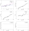 |
Fig. 4. Model fitting results for knot K09: Case 1. |
It can be seen that the observed trajectory and core separation versus time are well model-fitted, except for the zigzag section. Its bulk Lorentz factor is assumed to be Γ = constant = 16. Due to the viewing angle almost being constant, θ∼ = 1.25°, its Doppler factor and apparent velocity are derived to be δ ∼ 28.5 and βa ∼ 10.0c, respectively. These values are extremely consistent with those given by Jorstad et al. (2013): Γ = 15 ± 2, θ = 1.35 ± 0.2 (deg), δ = 27 ± 3, and βa = 9.6 ± 0.6c. Its observed precessing common trajectory is assumed extending to a core separation of rn ∼ 0.40 mas, equivalent to a spatial distance of Zc, p ∼ 141 pc (or Zc, m ∼ 18.3 mas) from the core. Therefore, the kinematic behavior of knot K09 can be well explained in terms of our precessing nozzle scenario.
In addition, we would like to suggest that the zigzag section of its trajectory could be caused by disturbances in jet-B, which might affect the VLBI modeling of the apparent motion of knot K09. Thus the exclusion of the zigzag trajectory section in the model-fitting may be valid.
3.5.2. Case 2: Model with zigzag trajectory section included
Here we also present the model-fitting results of the kinematics of knot K09 with the inclusion of the zigzag trajectory section, which are shown in Fig. 5. Its precession phase and ejection epoch are modeled as follows: ϕ0(rad) = 5.13 + 2π and t0 = 2009.66, which is about ∼120 days before the peak of the associated optical flare.
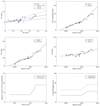 |
Fig. 5. Model fitting results for knot K09: Case 2. |
It can be seen that the observed trajectory is well fitted by the precessing nozzle model with most data points being within the region limited by the two lines (in magenta and blue) defined by precession phases 5.13 ± 0.31 rad. The core-separation and coordinates versus time are also well fitted (upper left and middle right panels in Fig. 5). Thus the kinematic behavior of knot K09 can be fully explained in terms of the precessing nozzle scenario for jet-A. Its observed precessing common trajectory may be regarded as extending to rn ∼ 0.40 mas, corresponding to a spatial distance of Zc, p ∼ 142.3 pc (or Zc, m ∼ 18.5 mas) from the core.
The proper motion of knot K09 increases along the jet and intrinsic acceleration is modeled as follows: for Z ≤ 10, Γ = 14.0; for Z = 10−15 mas, Γ = 14.0 + 8.8(Z − 10)/(15−10); and for Z > 15 mas, Γ = 22.8. During the period from 2009.8–2011.8, its bulk Lorentz factor Γ, Doppler factor δ, apparent velocity βa, and viewing angle θ approximately vary over the following respective ranges: [14.0 → 22.8]; [25.6 → 36.9], [7.7 → 17.9]c, and [1.24 → 1.22](deg).
3.6. Model fitting of kinematics of knot K14
We consider the following two cases: (1) K14 was ejected from the radio core at t0 = 2013.76 and (2) K14 was ejected from the optical core at 2013.76. The optical core is assumed to be at coordinates (Xn = −0.039 mas and Zn = −0.022 mas).
3.6.1. Case 1: K14 ejected from radio core, t0 = 2013.76
Its observation data were collected from Liodakis et al. (2020), where the core separation rn(t) and the average position angle PA = 61 ± 10 (deg) are given, implying a nonballistic motion. The model-fitting results of the kinematics of knot C14 are shown in Fig. 6. We assume that its precession phase is ϕ0(rad) = 1.30 + 4π, corresponding to the ejection epoch t0 = 2013.76.
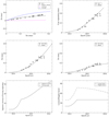 |
Fig. 6. Model fitting results for knot K14: Case 1. |
It can be seen that the kinematic behavior of knot K14 can be well explained in terms of the precessing nozzle model. Its precessing common trajectory was observed within rn ∼ 0.60 mas, corresponding to a spatial distance of Zc, p ∼ 759 pc (or Zc, m ∼ 98.7 mas) from the core.
Its motion is apparently accelerated with the apparent velocity increases from ∼15c to ∼27c during the period from 2014.6–2015.6, which is consistent with the average value (22.09 ± 0.14)c given in Liodakis et al. (2020). Its bulk Lorentz factor is modeled as follows: for Z ≤ 4 mas, Γ = 20.0; for Z = 4−15 mas, Γ = 20 + 15(Z − 4)/(15−4); for Z = 15−20 mas, Γ = 35 + 5(Z − 15)/(20−15); and for Z > 20 mas, Γ = 40. During the period from 2014.6–2015.6, its bulk Lorentz factor Γ, Doppler factor δ, apparent velocity βa, and viewing angle θ vary over the following respective ranges: [40 = constant], [77.2 → 69.7], [14.8 → 26.9]c, and [0.27 → 0.55](deg.). Thus its apparent acceleration is due to its motion along a curved trajectory, not due to intrinsic acceleration.
We point out that according to our precession nozzle model, the ejection epoch t0 = 2013.76 was earlier than those given by Traianou et al. (2018; t0 = 2014.3 ± 0.2) and Liodakis et al. (2020; t0 = 2014.38 ± 0.04). However, it is near the starting time of the associated optical flaring event with a slow rising phase and thus the ejection epoch derived by us seems quite reasonable because radio knot K14 could be the counterpart that evolved from the optical knot producing the optical flare (a shock through the optical core or injection of magnetized plasmas into the jet). This is consistent with the suggestion that one shock produces two flares: one optical and one radio knot ejection (Liodakis et al. 2020). Moreover, both are associated with optical and γ-ray outbursts.
It is worth noting that the position angle range 61 ± 10 (deg) is fully covered by the red and blue lines within core separation rn ∼ 0.6 mas, thus its observed trajectory is well explained by our precessing nozzle model.
3.6.2. Case 2: t0 = 2003.76, knot K14 ejected from the optical core
The precession phase is the same, ϕ0 = 1.30 + 4π, but the separation from the optical core should be corrected by 0.045 mas with respect to the radio core. In Fig. 7 we give the model-fitting results, assuming that knot K14 was ejected from the optical core (assumed at coordinates (−0.039 mas, −0.028 mas)) at ∼2013.76 and moving through the radio core at ∼2014.3. The apparent velocity and bulk Lorentz factor were similarly modeled.
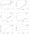 |
Fig. 7. Model fitting results for knot K14: Case 2. |
Its bulk Lorentz factor is assumed as follows: for Z ≤ 4 mas, Γ = 23.0; for Z = 4−15 mas, Γ = 23 + 12(Z − 4)/(15−4); for Z = 15−20 mas, Γ = 35 + 5(Z − 15)/(20−15); and for Z > 20 mas, Γ = 40. During the period from 2014.6–2015.6, its Lorentz factor Γ, Doppler factor δ, apparent velocity βa, and viewing angle θ vary over the following respective ranges: [40 = constant], [76.8 → 68.3], [15.5 → 28.2]c, and [0.29 → 0.59](deg.). Thus its apparent acceleration is due to its motion along a curved trajectory, not due to intrinsic acceleration.
In summary we emphasize that the detection of knot K14 is of great significance for our precessing nozzle model for jet-A, because the inclusion of its ejection at 2013.76 has extended the time interval for the model fitting of the nozzle precession in jet-A to ∼15 years, which is almost 1.5 times the precession period.
3.7. A brief summary for jet A
Based on our precessing nozzle scenario, we have consistently model-fitted the kinematic behaviors of six superluminal knots (B4, B5, K2, K3, K09, and K14), which are assumed to be ejected from jet-A. The detection of knot K14 is important, extending the model-fit over a time interval of ∼15 years, which is almost one and a half of the precession period 10.5 yr.
The model fitting results are summarized in Table 1, where the following model parameters for jet-A are presented: precession phase ϕ0(rad), ejection time t0(year), extension of the precessing common trajectory rn, c(mas), corresponding spatial distances Zc, m(mas) and Zc, p(pc), bulk Lorentz factor Γ, Doppler factor δ, apparent velocity βa(c), and viewing angle θ(deg).
Model parameters for the six superluminal knots (B4, B5, K2, K3, K09, and K14) of jet-A.
It is worth noting that the concept of the precessing common trajectory allowed us to model-fit the trajectories of these knots and their kinematic parameters consistently (Lorentz factor, Doppler factor, apparent velocity, and viewing angle versus time) were derived. Thus the kinematic behaviors of the knots can now be physically connected to the jet precession and the properties of the central engine. These results may be helpful to concretely study the physical parameter connection between the ejection of radio knots and their associated optical and γ-ray outbursts.
The extensions of precessing common trajectory for these knots are quite different, extending from a spatial distance of ∼60 pc (K3) to ∼750 pc (K14). This result needs to be tested using future VLBI observations.
4. Model fitting of the kinematics of jet B
Superluminal knots B1, B2, B3, B6, K1, K10, and K16 are assumed to be ejected by the nozzle of jet-B. In our scenario, the jet axis is defined in the (X, Y)-plane by parameters (ϵ,ψ) and formulas (1) and (2) in Sect. 2. Here for jet-B, we assume the following8: ϵ = 0.0126 rad (0.72°) and ψ = 0.20 rad (11.46°). ζ = 2, p1 = 0, p2 = 1.34 × 10⁻⁴mas−1, zt = 66 mas, and zm = 6.0 mas. The amplitude of the common helical trajectory is assumed to be A = A0[sin(πz0/Z1)]1/2, with A0 = 0.182 mas and Z1 = 396 mas. The phase of the helical trajectory is assumed to be ϕ = ϕ0-(z0/Z2)1/2 with Z2 = 3.58 mas. Furthermore, ϕ0 = ϕ(t0) is the precession phase of a knot, and t0 is its corresponding ejection time.
The parameters given above define the pattern of the spatial helical trajectory for jet-B, which precesses to produce the trajectory of individual knots at their corresponding precession phases. The precession phase of a knot is related to its ejection time as follows:
where T0 = 10.5 yr is the precession period of the jet-B nozzle.
When the parameters of the precessing nozzle scenario for jet-B are given as described above, we can then perform model-fitting of the observed kinematic behavior for each knot of jet-B and derive its bulk Lorentz factor and Doppler factor.
It is found that jet-B has a very small cone angle of ∼0.5° in space, but its projection in the plane of sky has a cone aperture of ∼36° with its jet axis at a position angle of ∼−101.5°, which differs from the position angle of jet-A by ∼17°. The modeled distribution of precessing common trajectories is shown in Fig. 8 (upper panel) and the observed trajectories of knots (B3, K1, and K10) are also shown for comparison. We find that most of the superluminal knots follow the precessing common trajectory defined above at different core separations.
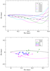 |
Fig. 8. Jet B: modeled distribution of precessing common trajectory (upper panel) and the observed trajectories of knots B3, K1, and K10 for comparison. |
4.1. Model fitting of kinematics of knot B1
Superluminal knots B1, B2, and B3 were ejected from the core at a similar position angle PA ∼ −80° (Jorstad et al. 2001). However, only knot B2 has been observed within a core separation of ∼0.15 mas. Thus we have to use the trajectory of knot B2 as a guide for making model-fitting of the kinematics for knots B1 and B3.
For knot B1, we assume the ejection time of t0 = 1994.46 derived by linear extrapolation of the core separation to zero (Jorstad et al. 2001), corresponding to precession phase ϕ0 = 0.42 rad. The model fitting results are shown in Fig. B.1.
Its precessing common trajectory was not observed and is assumed to extend to rn ∼ 0.07 mas, corresponding to a spatial distance of Zc, m ∼ 3.73 mas (or Zc, p ∼ 28.7 pc) from the core. Beyond this core separation, a change in parameter ψ is introduced to model-fit its outer trajectory as follows: for Z ≤ 5 mas, ψ = 0.20 rad; for Z = 5−15 mas, ψ(rad) = 0.20−0.65(Z − 5)/(15−5); and for Z > 15 mas, ψ = −0.45 rad.
No acceleration is assumed and its bulk Lorentz factor Γ = constant = 32.0. During the period from 1995.0–1995.5, its Doppler factor δ, apparent velocity βa, and viewing angle θ vary over the following ranges respectively: [50.4 → 58.9], [26.2 → 17.3]c, and [0.93 → 0.53](deg).
4.2. Model fitting of the kinematics of knot B2
Its ejection time is assumed to be t0 = 1994.90, which is consistent with what was derived by Jorstad et al. (2001), and precession phase is ϕ0 = 0.68 rad. The model-fitting results are shown in Fig. 9.
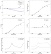 |
Fig. 9. Model fitting results for knot B2. |
Fortunately, the first data point plays a significant role, indicating that its initial trajectory could be fitted by the precessing nozzle model. But its observed trajectory beyond Xn ≃ 0.13 mas could only be explained by introducing a change in parameter ψ: for Z ≤ 5 mas, ψ = 0.20 rad; for Z = 5−15 mas, ψ(rad) = 0.20−0.35(Z − 3)/(15−5); and for Z > 15 mas, ψ = −0.15 rad.
Both acceleration and deceleration in its motion are assumed in the model fitting. The bulk Lorentz factor is assumed as follows: for Z ≤ 5 mas, Γ = 17; for Z = 5−15 mas, Γ = 17 + 17(Z − 5)/(15−5); for Z = 15−20 mas, Γ = 34−6(Z − 15)/(20−15); and for Z > 20 mas, Γ = 28. During the period from 1995.2–1997.0, its Lorentz factor Γ, Doppler factor δ, apparent velocity βa, and viewing angle θ vary over the following ranges respectively: [17.0–(33.9)–28.0], [31.0–(52.8)–51.7], [9.6–(28.3)–14.9]c, and [1.04–(0.50)–0.59](deg). Its observed precessing common trajectory is assumed extending to about core separation rn = 0.06 mas, which is equivalent to a spatial distance of Zc, m ∼ 3.47 mas (or Zc, p ∼ 26.7 pc) from the core.
4.3. Model fitting of the kinematics of knot B3
The model fitting results of the kinematics of knot B3 are shown in Fig. B.2. Its precession phase is ϕ0 = 1.10 rad and ejection time is t0 = 1995.60, consistent with what was derived by Jorstad et al. (2001). Its kinematics can be well fitted in terms of the precessing nozzle scenario and the observed precessing common trajectory is assumed to approximately extend to a core separation of 0.30 mas, which is equivalent to a spatial distance of Zc, m ∼ 18.7 mas (or Zc, p ∼ 143.8 pc) from the core. Its bulk Lorentz factor is modeled as Γ = const. = 14.0. During the period from 1996.5–1997.8, its Doppler factor δ, apparent velocity βa, and viewing angle θ approximately vary over the following ranges respectively: [26.4–26.6], [6.5–6.1]c, and [1.01–0.94](deg). They almost stay constant.
4.4. Model-fitting of the kinematics of knot B6
The model fitting results for knot B6 are shown in Fig. 10. We assume that its ejection time t0 = 1999.61, which is consistent with what is given by Jorstad et al. (2005; t0 = 1999.80 ± 0.37), and the corresponding precession phase ϕ0 = 3.50 rad.
 |
Fig. 10. Model fitting results for knot B6. |
Within Xn ≃ 0.5 mas, the observed curved trajectory was fitted because the data points are all in the region defined by the magenta and blue lines9. Similar initial trajectory curvature also occurred in the motion of knot K10 (see below), indicating the repeat performance of the phenomenon.
A remarkable feature observed for B6 is its accelerated motion. We model-fit its bulk Lorentz factor as follows: for Z ≤ 10 mas, Γ = 22; for Z = 10−20 mas, Γ = 22 + 13(Z − 10)/(20−10); and for Z > 20 mas, Γ = 35. During the period from 1999.8–2001.3, its bulk Lorentz factor Γ, Doppler factor δ, apparent velocity βa, and viewing angle θ vary over the respective ranges: [22.0, 35.0], [43.0, (57.1), 48.7], [6.4, 32.2]c, and [0.39, 1.08](deg.). These values are well compared with those derived by Jorstad et al.: Γ = 25.27, δ = 29.7, βa = 24.8 ± 2.5c, and θ = 1.9°.
Its observed precessing common trajectory is assumed to extend to a core separation of rn ∼ 0.7 mas, which is equivalent to a spatial distance of Zc, m ∼ 51.7 mas (or Zc, p ∼ 397.8 pc) from the core.
The model fitting of the kinematics of knot B6 seems quite successful, demonstrating that our precessing nozzle scenario is valid for jet-B. Below we show that the successful model fitting of the kinematics for knot K10 further verifies the assumed double-jet scenario for 3C454.3 and the precessing nozzle model for jet-B.
4.5. Model fitting of kinematics of knot K1
For the model-fitting of the kinematics of knot K1, we consider two cases. First, its ejection time is assumed to be 2005.50 adopted from Jorstad et al. (2010), which corresponds to a precession phase of ϕ0 = 0.74 + 2π. This ejection time is after the peaking of the associated optical flare. Second, the ejection time is assumed to be t0 = 2004.29, corresponding to a precession phase of ϕ0 = 0.02 + 2π. This ejection time is near the beginning of the slowly rising phase of the associated optical flare (Jorstad et al. 2010).
4.5.1. Case 1: Model fitting of kinematics of knot K1 with t0 = 2005.50
The ejection time t0 = 2005.50 is after the peaking of the associated optical flare (Jorstad et al. 2010). The model-fitting results are shown in Fig. B.3. In this case the observed trajectory departs from the predicted precessing common trajectory (defined by the region limited by the magenta and blue lines in Fig. B.3), and we introduced the following changes in parameter ψ to fit the observed trajectory: for Z ≤ 3 mas, ψ = 0.2 rad; for Z = 3−5 mas, ψ(rad) = 0.2 + (Z − 3)(0.4−0.2)/(5−3); and for Z > 5 mas, ψ = 0.40 rad. We assume its bulk Lorentz factor = constant = 12.0. During the period from 2006.0–2007.4, its Doppler factor δ, apparent velocity βa, and viewing angle θ vary over the following ranges respectively: [22.9 → 23.0], [4.0 → 4.7]c, and [1.03 → 0.97](deg). Its observed precessing common trajectory is modeled as extending to a core separation of rn≃0.06 mas, which is equivalent to a spatial distance of Zc, m ∼ 3.47 mas (or Zc, p ∼ 26.7 pc) from the core.
4.5.2. Case 2: Model fitting of kinematics of knot K1 with t0 = 2004.29
The ejection time t0 = 2004.29 is near the beginning of the slowly rising phase of the associated optical flare, implying that the optical flare is possibly due to knot K1 passing through a stationary shock in the optical jet. In this case the observed trajectory can be well fitted by the predicted precessing common trajectory. This result seems important for investigating the connection of its multiwavelength variability from radio and optical to high-energy γ-rays.
The model fitting results are shown in Fig. B.4. Its motion is modeled as accelerated. The bulk Lorentz factor is assumed as follows: for Z ≤ = 1.0 mas, Γ = 5; for Z = 1−5 mas, Γ = 5 + (Z − 1)(12.5−5)/(5−1); and for Z > 5 mas, Γ = 12.5. During the period from 2006.0-2007.5, its Lorentz factor Γ, Doppler factor δ, apparent velocity βa, and viewing angle θ vary over the following ranges respectively: [8.6 → 12.5], [16.7 → 24.1], [2.7 → 4.4]c, and [1.09 → 0.84](deg). Its observed precessing common trajectory is assumed to approximately extend to a core separation of rn ≃ 0.20 mas, which is equivalent to a spatial distance of Zc, m ∼ 11.5 mas (or Zc, p ∼ 88.2 pc) from the core.
Here we would like to point out that the millimeter outburst associated with the ejection of knot K1 revealed a multiple-peak structure (Krichbaum et al. 2008), similar to what was observed in optical bands (Jorstad et al. 2010). Krichbaum et al. assembled the millimeter-radio spectra at different times for this outburst, showing its complex spectral evolution, which would need to be interpreted in connection with the evolution of the optical emission because these spectra may be composed by the emissions from different regions in the curved jet (Raiteri et al. 2012; D’Arcangelo et al. 2009).
4.6. Model-fitting of the kinematics of knot K10
Superluminal knot K10 is an extremely important superluminal component for our scenario. And it is associated with an exceptionally strong high-energy (> 100 MeV) γ ray outburst with its peak flux density reaching six times the flux density of the Vela pulsar.
As we have mentioned that the curved trajectory of K10 almost repeated that of knot B6, exhibiting a significant signal for the periodicity in ejection of superluminal components in 3C454.3.
We consider the following two cases: (1) the ejection time t0 = 2010.95, which is consistent with what is given in Jorstad et al. (2013); and (2) the ejection time t0 = 2010.80, concordant with the start of the associated optical flare. The observed kinematics of knot K10 can be model-fitted well in both cases.
4.6.1. Case 1: t0 = 2010.95
The model-fitting results are shown in Fig. 11. It can be seen that the entire kinematic behavior has been model-fitted very well by our precessing jet-nozzle scenario.
-
The ejection time of K10 is considered to be t0 = 2010.95 (corresponding precession phase ϕ0(rad) = 4.0 + 2π), which is fully consistent with 2010.95 ± 0.07 given in Jorstad et al. (2013).
-
According to Jorstad et al., knot K10 appears at a position angle (PA) ≈−136° and then its trajectory curves into the direction of PA ≈ −92°. Our model fitting results give the position angle = −138° (at a core separation of rn = 0.05 mas) and PA = −91° (at rn = 0.4 mas). Thus our model completely explains the curved trajectory of knot K10. Its observed precessing common trajectory is assumed to extend to a core separation of rn ∼ 0.22 mas, which is equivalent to a spatial distance of Zc, m ∼ 23.7 mas (or Zc, p ∼ 182.5 pc) from the core.
-
For the period from 2011.1–2011.8, its bulk Lorentz factor is modeled as Γ = 25.0 = const., compared with Γ = 26 ± 3 given in Jorstad et al.
-
The corresponding Doppler factor δ varies in the range [47.9, 45.9], compared with 51 ± 4 given by Jorstad et al.
-
Its apparent velocity βa varies in the range [4.9, 13.7], compared with βa = 8.9 ± 1.7 given by Jorstad et al.
-
We obtain its viewing angle θ varying in the range [0.47, 0.68](deg), compared with the value θ = 0.4° ± 0.1° given in Jorstad et al.
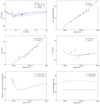 |
Fig. 11. Case 1: Model fitting results for knot K10. |
Therefore, the kinematic parameters we modeled for K10 are quite consistent with those given in Jorstad et al. (2013). Our precessing nozzle scenario and the model-fitting results for knot K10 are valid and effective.
4.6.2. Case 2: t0 = 2010.80
The model fitting results are shown in Fig. 12. It can be seen that the observed kinematics of knot K10 can also be model-fitted well. The modeled Lorentz factor Γ = constant = 22.5 is a bit smaller than that taken for case 1 (Γ = 25.0). During the period from 2011.10–2011.80, its Doppler factor δ, apparent velocity βa, and viewing angle θ vary over the respective ranges: [43.8, 41.9], [7.2, 11.4]c, and [0.42, 0.69](deg). Its observed precessing common trajectory is assumed to extend to a core separation of rn ∼ 0.22 mas, equivalent to a spatial distance of Zc, m ∼ 23.5 mas (or Zc, p ∼ 180.5 pc) from the core.
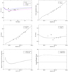 |
Fig. 12. Case 2: Model fitting results for knot K10. |
The full fitting of the kinematics of knot K10 with an ejection time of t0 = 2010.80 may be meaningful because in some physical conditions radio knots can be regarded as the evolved counterpart of optical knots. In fact, the ejection time t0 = 2010.95 was derived by linear extrapolation to zero separation from the core, being a “mathematical solution”, while the ejection time t0 = 2010.80 was derived from the connection between optical and radio outbursts, being a “physical solution”. Here we show that both solutions are possible.
However, its outbursts at 1 mm and optical wavebands simultaneously peaked at ∼2455520.657, which seems to imply that knot K10 was ejected before 2010.95 ± 0.07 (2455543 ± 25).
4.7. Model fitting of kinematics of knot K16
Its observational data were collected from Weaver et al. (2019): the core separation rn(t) and average position angle PA = −79 ± 1 (deg.). Thus K16 moves ballistically.
At first sight, the analysis of the kinematics of knot K16 was difficult because no observational data were available within a core separation of ∼0.15 mas and no appropriate solution could be found for fitting its observed trajectory. It was not clear whether knot K16 was associated with jet-A or jet-B. However, we at last found that its trajectory section between Xn(mas) = (0.15, 0.25) is well concordant with that of the observed trajectory of knot B2, as shown in Fig. 13. This clue was quite important and showed us that knot K16 should belong to jet-B and its initial kinematic behavior should be fitted with a precession phase of ϕ0 ≃ 0.68 + 4π and corresponding ejection epoch of t0 ≃ 2015.90, which is exactly equal to 1994.90 (t0 for knot B2) plus 21.0 yr (two precession periods). This result is very instructive and encouraging when searching for the periodicity in 3C454.3 through VLBI observations of superluminal components.
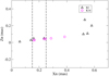 |
Fig. 13. Similarity of the trajectory sections of knot K16 and B2 between Xn = 0.15 mas and 0.25 mas. This comparison provides a rather important clue, showing that the kinematic behavior of knot K16 should be explained similarly to that of knot B2; an open circle corresponds to K16 and an open triangle corresponds to B2. |
The model-fitting results of the kinematics of knot K16 are shown in Fig. 14. Its observed precessing common trajectory is assumed to extend to ∼0.10 mas, which is equivalent to a spatial distance of Zc, m ∼ 5.87 mas (or Zc, p ∼ 45.1 pc) from the core.
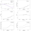 |
Fig. 14. Model fitting results for knot K16. |
Its outer trajectory can be fitted by introducing changes in parameter ψ: for Z ≤ 5 mas, ψ = 0.20 rad; for Z = 5–15 mas, ψ(rad) = 0.20−0.35(Z − 5)/(15−5); and for Z > 15 mas, ψ = −0.15 rad.
Its bulk Lorentz factor is modeled as follows: for Z ≤ 5 mas, Γ = 17; for Z = 5–15 mas, Γ = 17 + 15(Z − 5)/(15−5); and for Z > 15 mas, Γ = 32.
During the period from 2016.4–2017.2, the bulk Lorentz factor increases from 18.7 to 32.0 and the modeled apparent velocity βa varies over the range [11.3, (25.8, maximum), 21.6], which is consistent with what is given by Weaver et al. (2019; 20.3 ± 0.8). However, our modeled Doppler factor δ varying over the range [33.6–55.6] is much higher than what was derived from the observed minimum variability timescale (∼2 hr) in Weaver et al. (δ = 22.6). In our model, its viewing angle varies over the range [1.03, 0.69](deg). Thus we reach the conclusion that the kinematics of knot K16 can be explained well in terms of our precessing nozzle scenario for jet-B with a precession period of 10.5 yr.
4.8. A brief summary for jet B
Seven knots (B1, B2, B3, B6, K1, K10, and K16) were ejected from jet-B. Their kinematic behavior can be explained well and model-fitted in terms of our precessing nozzle scenario for jet-B. The model fitting results are summarized in Table 2, where the following model parameters for jet-B are presented: precession phase ϕ0(rad), ejection time t0(year), extension of the precessing common trajectory rn, c(mas), corresponding spatial distances Zc, m(mas) and Zc, p(pc), bulk Lorentz factor Γ, Doppler factor δ, apparent velocity βa(c), and viewing angle θ(deg).
Model parameters for the seven superluminal components (B1, B2, B3, B6, K1, K10, and K16) of jet-B.
The most prominent features of jet B are the presence of two pairs of knots, B6-K10 and B2-K16. In the case of pair B6-K10, they have similar ejection position angles and similar curved initial trajectories with a difference in ejection times of ∼11.2 yr, which is close to a precession period of 10.5 yr. In the case of pair B2-K16, they have similar ballistic trajectories with a difference in ejection times of 21.0 yr, which is exactly equivalent to two precession periods. We emphasize that this kind of repeated occurrences of similar ejection position angles and trajectory patterns are significant clues to find a precessing common trajectory and a precession period of a jet nozzle.
5. Discussion and conclusion
We have made use of our precessing nozzle scenario proposed previously (e.g., Qian et al. 1991, 2009, 2019) to model-fit the kinematic behavior of thirteen superluminal knots in blazar 3C454.3. The main results are as follows.
-
We show that blazar 3C454.3 might host a supermassive black hole binary, which produces two relativistic jets. Both jet nozzles precess with the same period of 10.5 yr and eject superluminal components steadily.
-
In this case, the observed superluminal components may be divided into the following two groups: group A (knots B4, B5, K2, K3, K09, and K14) and group B (knots B1, B2, B3, B6, K1, K10, and K16). The kinematics (trajectory, coordinates, and apparent velocity versus time) of the knots in group A and group B can then be well and consistently interpreted in terms of the precessing nozzle models for jet A and B, respectively. The kinematic parameters (Lorentz factor, Doppler factor, and viewing angle versus time) can be derived. Although for a few knots the model-fittings may have some uncertainties due to the lack of observational data, the kinematic behaviors of most knots have been well model-fitted, especially for those associated with strong γ-ray outbursts, for example for knots K09 and K10.
-
The key ingredient of our precessing nozzle scenario is the assumption about the presence of the precessing common trajectory. That is to say, all the superluminal knots move along the common trajectory, which precesses and produces the trajectory of individual knots ejected at different times (or at different precession phases). Based on this assumption, we then can consistently arrange the distribution of the trajectory of the knots ejected at different times and model-fit the kinematics of the superluminal knots and derive the period of jet-nozzle precession.
-
Interestingly, for the blazars and quasi-stellar objects (QSOs: 3C279, 3C454.3, OJ287, B1308+326, PG1302-102, and NRAO 150), we have applied the precessing nozzle scenario to interpret their VLBI kinematics and determine the periods of their jet-nozzle precession. We find that the assumption of a precessing common trajectory has been generally valid, but the observed pattern and the extension of a precessing common trajectory are quite different for different sources and different superluminal knots (readers can refer to Qian et al. 2019 and the references therein). Higher resolution VLBI observations are needed to show if this assumption is still valid within core separations < 0.1 mas.
-
This assumption could be based on the theoretical works of relativistic magnetohydrodynamics for jet-formation that magnetic effects in the acceleration and collimation zone of relativistic jets are very strong, forming some very solid magnetic structures and controlling the trajectory patterns of moving superluminal knots ejected from the jet nozzle (e.g., Vlahakis & Koenigl 2004; Blandford & Payne 1982; Blandford & Znajek 1977; Camenzind 1990 and references therein). Thus all the superluminal components in a blazar can move along the same (or common) steady trajectory, which precesses if the jet nozzle is precessing.
-
By means of model-fitting of the kinematics of the superluminal knots in blazar 3C454.3, we find that the precessing common trajectory can be observed for different knots over a range of core separation ∼(0.07 mas, 0.8 mas), corresponding to a range of spatial distance from the radio core of ∼(50, 800) pc. Obviously, VLBI observations with higher resolutions are required to confirm the observed common trajectory extending inward to the core.
-
In the process of model-fittings, we obtain the bulk Lorentz factor Γ versus time for the superluminal knots attributed to jet-A and jet-B: both intrinsic acceleration and deceleration in motion are found. For jet-A and jet-B, the derived Lorentz factor varies over ranges ∼[6, 40] and ∼[9, 32], respectively (see Tables 1 and 2). These values are model-dependent, but for the first time they provide some observational basis to investigate the physics of the relativistic jets on different scales in 3C454.3. Moreover, the derivation of Doppler factor for these superluminal knots may have provided the physical basis to investigate the mechanisms of their multiwavelength emission from radio and optical to high-energy γ-rays.
-
A prominent periodic phenomenon has been found in th ejection of superluminal components, being the recurrence of knot ejections along similar position angles. The following three pairs of knots remarkably show this effect: B2-K16, B4-09, and B6-K10. In particular, the pair B6-K10 not only reveals the similar curved trajectories, but it also shows their ejection times differing by 11.34 yr, which is close to a precession period of 10.5 yr. The pair B2-K16 have a similar trajectory and ejection times differing by 21 yr, exactly equal to two precession periods.
-
The recurrence of these distinct features as described above may be important instructive signatures for recognizing jet-nozzle precession in 3C454.3 and other blazars and would be very helpful to analyze the physical processes (jet formation, radiation, and motion of superluminal knots) in blazars. In particular, the observed recurrence of trajectory patterns may be the best piece of evidence for periodicity in blazars. In addition, if the suggestion of the presence of supermassive binary black hole systems in some blazars is confirmed, the currently available physical concepts and observational data analysis methods based on a single-jet scenario for studying blazars will be greatly challenged.
-
Based on the observed apertures of the precessing cones for jet-A and jet-B, the mass ratio of the binary black hole can be estimated to be q = m/M ∼ 0.3. Combining this mass ratio with the known measurements of the hole mass M (e.g., Woo & Urry 2002; Gu et al. 2001), we can approximately estimate the separation rpc between the binary holes and the post-Newtonian parameter ϵn (Qian et al. 2017, 2018). For M = (1.6−4.4)×109 M⊙, rpc = 2.1–2.9 and ϵn = (4.8-9.4) × 10−3, which is approximately comparable with the critical value ϵn = 0.01, indicating that the motion of the secondary hole is near relativistic. As in the case of OJ287, the interpretation of VLBI kinematics in terms of our precessing nozzle scenario may be helpful for deriving the parameters of orbital motion in supermassive black hole binaries (Qian 2018).
On the whole, now we can understand the entire kinematics and dynamics obtained by VLBI observations in 3C454.3, including its peculiar features. First, a putative supermassive binary black hole creates two relativistic jets (jet A and jet B). Second, the two jets alternately eject superluminal components: Jet-B (knots B1, B2, and B3) → Jet-A (knots B4 and B5) → Jet-B (knots B6 and K1) → Jet-A (knots K2, K3, and K09) → Jet-B (knot K10) → Jet-A (knot K14) → Jet-B (knot K16). This is a very interesting phenomenon and will become a great challenge to physics of blazars if confirmed in future observations. Third, the axes of jet-A and jet-B have different directions in space and are defined by parameters (ϵ, ψ) (in radians): (0.0126, −0.1) and (0.0126, +0.20), respectively, referring to Fig. 1. Jet-A has its apparent axis at a position angle of PA ≃ −84° and jet-B at PA ≃ −101°. Their nozzle-precessing cones have half opening angles ≃30° (jet-A) and ≃10° (jet-B). The ejections of superluminal components in such wide cones lead to the wide distribution of the knots’ trajectories, as shown by knots R1, R2, R3, and R4 observed at 15 GHz (Britzen et al. 2013). Fourth, these knots and the associated shocks due to an interaction with the surrounding interstellar medium apparently form a ring-like structure (a prominent feature of 3C454.3) surrounding the core (Britzen et al. 2012). Fifth, the trajectories of these knots on the ring-like structure may have been reconverged at coordinate Xn ≃ 3 mas, constructing a second nozzle to eject the magnetized plasmas which then move along the direction toward knots Y and Z at core distances ∼10 mas (Qian et al. 2014). Sixth, due to the formation of stationary shocks in the jets, the peculiar phenomenon of “superluminal brightening and expanding” observed by Pauliny-Toth et al. (1987), Pauliny-Toth (1998) can be well understood, while superluminal components may be associated with the traveling shocks, as is usually suggested. Seventh, the superluminal components ejected from both the jets and their evolution may become the main causes producing the extremely complex and violent variability across the entire electromagnetic spectrum from radio to high energy γ-rays and the periodic behaviors in the light curves.
Our precessing nozzle scenario for blazar 3C454.3 is tentative and needs to be tested by future VLBI observations because the phenomena occurred in this blazar are exceptionally complex. For example, as shown by Britzen et al. (2012), the kinematic behavior of the superluminal components could be affected (or governed) by several different ingredients: jet precession and nutation, the rotation of knots, the formation of both stationary and traveling shocks, the formation of a superluminally expanding ring-like structure and jet recollimation and reopening (Qian et al. 2014), and an interaction between a jet and surrounding medium. In other blazars, similar complex phenomena have been observed and investigated, for example, in 3C279 (Qian 2011, 2012; Qian et al. 2019) and OJ287 (Qian 2018, 2019a,b, 2020).
Until know we have shown that blazar 3C279 (Qian et al. 2019), OJ287 (Qian et al. 2018; Britzen et al. 2018), and 3C454.3 (this paper, Qian et al. 2007, 2014) could host putative binary black holes. We have also made use of our precessing nozzle scenario to interpret the kinematics of the superluminal components in a few QSOs and determine their jet-nozzle precession periods, including, for example, the following: QSOs 3C345, B1038+326, PG1302-102, and NRAO 150 (Qian et al. 2009, 2017; Qian 2018, 2016).
We would like to point out that our precessing nozzle scenarios for these blazars and QSOs are not only based on the model fittings of available VLBI data, but they have also been verified by other observations. For example, in the case of OJ287, Hodgson et al. (2017) found some evidence for the possible presence of two ejection directions in OJ287. Particularly in the case of 3C279, one of the double jets (jet-B; Qian et al. 2019), which had been predicted and searched for quite a long time, had been found to be already observed much earlier (Pauliny-Toth et al. 1987; Pauliny-Toth 1998; de Pater & Perley 1983; Cheung 2002).
These investigations may have confirmed the assumption about the presence of the precessing common trajectory. Moreover, the proposed double precessing nozzle mechanism may be a great challenge to blazar physics based on a single-jet structure. Especially, in the case of blazar OJ287, there could be a possibility that the quasi-periodicity of ∼12 yr found in its optical light curve (Sillanpää et al. 1988, 1996; Lehto & Valtonen 1996) might be interpreted in terms of a double-jet mechanism (Qian et al. 2018; Qian 2019a,b, 2020; also referring to Villata et al. 1998; Qian et al. 2007)10. Magnetohydrodynamic (MHD) theories for double-jet formation in binary black hole systems involve very complex physical processes (including the spin of holes, the accretion of mass and magnetic fields, the formation of magnetospheres as well as the effects of general relativity (Einstein 1916, 1918)). Thus the processes producing quasi-periodicities in dual-jet systems have not been widely studied (e.g., Shi et al. 2012; Shi & Krolik 2015; Artymovicz & Lubow 1996; Artymovicz 1998; D’Orazio et al. 2013; Tanaka 2013 and references therein), although supermassive black hole binaries have already been assumed as a hopeful scenario to explain the quasi-periodic behavior observed in blazar OJ287 (e.g., Artymovicz 1998). Particularly, Shi & Krolik (2015) argued that in the MHD framework, cavity-accretion rates can be raised to make both black holes producing a jet and forming a double jet system.
In conclusion, we suggest that blazar 3C454.3 could host a binary black hole system in its nucleus. Similar systems have been suggested for blazar 3C279 (Qian et al. 2019) and blazar OJ287 (Britzen et al. 2018; Qian et al. 2018). Although these scenarios are only hypothetical and putative, not unique, and have yet to be tested, they could be useful for understanding the superluminal phenomena in blazars and for disentangling different mechanisms and ingredients. Due to the consistency of the model-fitting results of VLBI kinematics for three blazars, our precessing nozzle scenario might be actually applicable.
As suggested by Vercellone et al. (2011) that for explaining the extreme γ-ray variability and the spectral energy distributions observed in 3C454.3, an intriguing possibility is to invoke the presence of a supermassive binary black hole as previously hypothesized in Qian et al. (2007). Here in this paper we perhaps have really provided possible evidence for such a system in 3C454.3. However, we should emphasize that this work cannot exclude single-jet scenarios with or without a precessing jet-nozzle and more observational data on the kinematics in the innermost jet regions (especially at core separations of rn < 0.05–0.1 mas) are needed to solve the issues.
Jorstad et al. (2005) derived δ and θ from flux variability timescales.
It is noted that both the optical flares respectively associated with knots K2 and K3 have slowly rising phases before reaching their flaring peaks (Jorstad et al. 2010).
In a recent work, Qian (2020) investigated the polarization properties of the quasi-periodic optical outbursts observed in 1984, 2007, and 2015 in OJ287 and demonstrate that they may originate from synchrotron radiation (not from bremsstrahlung) due to the presence of large polarization angle swings, which is consistent with the results for the 1984 outburst obtained by Holmes et al. (1984). Thus these optical outbursts may likely be produced in its double relativistic jets. Kushwaha (2020) recently argued that the bremsstrahlung of the 3 × 10⁵ K gas bubble as suggested in the impact-disk model (Valtonen et al. 2019) cannot explain the NIR, optical, and UV spectral variations. It seems that the various types of NIR and optical variations observed in OJ287 may likely be understood in terms of multi-emitting regions in its double optical relativistic jet (e.g., Bonning et al. 2012, 2010; Raiteri et al. 2007; Villata et al. 2006; Sillanpää et al. 1996).
Acknowledgments
Qian gratefully acknowledges the support of publishing fund from Max-Planck Institut für Radioastronomie. Qian would like to thank Ya-yuan Wen (National Astronomical Observatories of Chinese Academy Sciences) for her long-lasting help with preparation of our papers. Qian also thanks Jing-wen Qian for her help with making the figure describing the geometry of the precessing nozzle scenario.
References
- Abdo, A. A., Ackermann, M., Ajello, M., et al. 2009, ApJ, 699, 817 [NASA ADS] [CrossRef] [Google Scholar]
- Abdo, A. A., Ackermann, M., Agudo, I., et al. 2010, ApJ, 716, 30 [NASA ADS] [CrossRef] [Google Scholar]
- Abdo, A. A., Ackermann, M., Ajello, M., et al. 2011, ApJ, 733, L26 [NASA ADS] [CrossRef] [Google Scholar]
- Artymovicz, P. 1998, in Theory of Black Hole Accretion Disks, eds. M. A. Abramowicz, G. Björnsson, & J. E. Pringle, 202 [Google Scholar]
- Artymovicz, P., & Lubow, S. H. 1996, ApJ, 467, L77 [NASA ADS] [CrossRef] [Google Scholar]
- Blandford, R. D., & Payne, D. G. 1982, MNRAS, 199, 883 [NASA ADS] [CrossRef] [Google Scholar]
- Blandford, R. D., & Znajek, R. L. 1977, MNRAS, 179, 433 [Google Scholar]
- Bonning, B. W., Bailyn, C., Urry, C. M., et al. 2009, ApJ, 697, L81 [NASA ADS] [CrossRef] [Google Scholar]
- Bonning, B. W., Bailyn, C., Urry, C. M., et al. 2010, in Accretion and Ejection in AGNs: A Global View, eds. L. Maraschi, G. Ghisellini, R. Della Ceca, F. Tavecchio, et al., ASP Conf. Ser., 427, 265 [NASA ADS] [Google Scholar]
- Bonning, B. W., Urry, C. M., Bailyn, C., et al. 2012, ApJ, 756, 13 [NASA ADS] [CrossRef] [Google Scholar]
- Bonnoli, G., Ghisellini, G., Foschini, L., et al. 2011, MNRAS, 410, 368 [NASA ADS] [CrossRef] [Google Scholar]
- Britzen, S., Zamaninasab, M., Aller, M., et al. 2012, J. Phys. Conf. Ser., 372, 012029 [NASA ADS] [CrossRef] [Google Scholar]
- Britzen, S., Qian, S. J., Witzel, A., et al. 2013, A&A, 557, A37 [NASA ADS] [CrossRef] [EDP Sciences] [Google Scholar]
- Britzen, S., Fendt, C., Witzel, G., Qian, S. J., et al. 2018, MNRAS, 478, 3199 [NASA ADS] [Google Scholar]
- Camenzind, M. 1990, Rev. Mod. Astron., 3, 234 [Google Scholar]
- Cheung, C. C. 2002, ApJ, 581, L15 [NASA ADS] [CrossRef] [Google Scholar]
- Daly, R. A., & Marscher, A. P. 1988, ApJ, 334, 539 [NASA ADS] [CrossRef] [Google Scholar]
- D’Arcangelo, F. D., Marscher, A. P., Jorstad, S. G., et al. 2009, ApJ, 697, 985 [NASA ADS] [CrossRef] [Google Scholar]
- de Pater, I., & Perley, R. A. 1983, ApJ, 273, 64 [NASA ADS] [CrossRef] [Google Scholar]
- Donnarumma, I., Pucella, G., Vittorini, V., et al. 2009, ApJ, 707, 1115 [NASA ADS] [CrossRef] [Google Scholar]
- D’Orazio, D. L., Haiman, Z., & Macfadyen, A. 2013, MNRAS, 436, 2997 [NASA ADS] [CrossRef] [Google Scholar]
- Einstein, A. 1916, Sitzungberichte der Königlich Presssichen Akademie der Wissenshafte (Berlin: SPAW), 688 [Google Scholar]
- Einstein, A. 1918, Sitzungberichte der Königlich Presssichen Akademie der Wissenshafte (Berlin: SPAW), 154 [Google Scholar]
- Finke, J. D., & Dermer, C. D. 2010, ApJ, 714, L303 [NASA ADS] [CrossRef] [Google Scholar]
- Foschini, L., Ghisellini, G., Tavecchio, F., et al. 2011, A&A, 530, A77 [NASA ADS] [CrossRef] [EDP Sciences] [Google Scholar]
- Fuhrmann, L., Cucchiara, A., Marchili, N., et al. 2006, A&A, 445, L1 [NASA ADS] [CrossRef] [EDP Sciences] [Google Scholar]
- Ghisellini, G., Foschini, L., Tavecchio, F., & Pian, E. 2007, MNRAS, 382, L82 [NASA ADS] [CrossRef] [Google Scholar]
- Giommi, P., Blustin, A. J., Capalbi, M., et al. 2006, A&A, 456, 911 [NASA ADS] [CrossRef] [EDP Sciences] [Google Scholar]
- Gomez, J. L., Marti, J. M., Marscher, A. P., et al. 1997, ApJ, 482, L33 [NASA ADS] [CrossRef] [Google Scholar]
- Gu, M., CaO, X., & Jiang, D. R. 2001, MNRAS, 327, 1111 [NASA ADS] [CrossRef] [Google Scholar]
- Hodgson, J. A., Krichbaum, T. P., Marscher, A. P., et al. 2017, A&A, 597, A80 [NASA ADS] [CrossRef] [EDP Sciences] [Google Scholar]
- Hogg, D. W. 1999, ArXiv e-prints [arXiv:astro-ph/9905116] [Google Scholar]
- Holmes, P. A., Brand, P. W. J. L., Impey, C. D., et al. 1984, MNRAS, 211, 497 [NASA ADS] [CrossRef] [Google Scholar]
- Jorstad, S. G., Marscher, A. P., Mattox, J. R., et al. 2001, ApJ, 556, 738 [NASA ADS] [CrossRef] [Google Scholar]
- Jorstad, S. G., Marscher, A. P., Lister, M. L., et al. 2005, AJ, 130, 1418 [NASA ADS] [CrossRef] [Google Scholar]
- Jorstad, S. G., Marscher, A. P., Larionov, V. M., et al. 2010, ApJ, 715, 362 [NASA ADS] [CrossRef] [Google Scholar]
- Jorstad, S. G., Marscher, A. P., Smith, P. S., et al. 2013, ApJ, 773, 147 [NASA ADS] [CrossRef] [Google Scholar]
- Jorstad, S. G., Marscher, A. P., Morozova, D. A., et al. 2017, ApJ, 846, 98 [NASA ADS] [CrossRef] [Google Scholar]
- Krichbaum, T. P., Lee, S. S., Lobanov, A. P., Marscher, A. P., & Gurwell,, M. A. 2008, in Extragalactic jets: Theory and Observation from Radio to Gamma Ray, eds. T. A. Rector, D. S. De Young, et al., ASP Conf. Ser., 386, 186, (San Francisco, CA) [NASA ADS] [Google Scholar]
- Kudryavtseva, N. A., & Pyatunina, T. B. 2008, Astron. Rep., 50, 1 [Google Scholar]
- Kushwaha, P. 2020, Galaxies, 8, 15 [CrossRef] [Google Scholar]
- Lehto, H. J., & Valtonen, M. J. 1996, ApJ, 460, 207 [NASA ADS] [CrossRef] [Google Scholar]
- Liodakis, L., Blinov, D., Jorstad, S. G., et al. 2020, ApJ, 902, 61 [NASA ADS] [CrossRef] [Google Scholar]
- Marscher, A. P. 2013, 2012 4th Fermi Symposium Proceedings eConf C121028, [arXiv:1304.2064] [Google Scholar]
- Meier, D. L., & Nakamura, M. 2006, in Blazar Variability Workshop II: Entering the GLAST Era, eds. H. R. Miller, K. Marshall, J. R. Webb, & M. F. Aller, ASP Conf. Ser., 350, 195 [NASA ADS] [Google Scholar]
- Ogle, P. M., Wehrle, A. E., Balonek, T., & Gurwell, M. A. 2011, ApJS, 195, 19 [NASA ADS] [CrossRef] [Google Scholar]
- Pacciani, L., Vittorini, V., Tavani, M., et al. 2010, ApJ, 716, L170 [NASA ADS] [CrossRef] [Google Scholar]
- Pauliny-Toth, I. I. K. 1998, in Radio Emission from Galactic and Extragalactic Compact Sources, eds. J. A. Zensus, G. B. Taylor, & J. M. Wrobel, ASP Conf. Ser., 114, 75 [Google Scholar]
- Pauliny-Toth, I. I. K., Porcas, R. W., Zensus, J. A., et al. 1987, Nature, 328, 778 [NASA ADS] [CrossRef] [Google Scholar]
- Pian, E., Foschini, L., Beckmann, V., et al. 2006, A&A, 449, L21 [NASA ADS] [CrossRef] [EDP Sciences] [Google Scholar]
- Pyatunina, T. B., Kudryavtseva, N. A., Gabuzda, D. C., et al. 2004, in Proc. of the all-Russia Astronomical Conference "Horizons of the Universe", Moscow, 109 [Google Scholar]
- Qian, S. J. 2011, Res. Astron. Astrophys., 11, 43 [NASA ADS] [CrossRef] [Google Scholar]
- Qian, S. J. 2012, Res. Astron. Astrophys., 12, 46 [NASA ADS] [CrossRef] [Google Scholar]
- Qian, S. J. 2016, Res. Astron. Astrophys., 16, 20 [NASA ADS] [CrossRef] [Google Scholar]
- Qian, S. J. 2018, ArXiv e-prints [arXiv:1811.11514] [Google Scholar]
- Qian, S. J. 2019a, ArXiv e-prints [arXiv:1904.03357] [Google Scholar]
- Qian, S. J. 2019b, ArXiv e-prints [arXiv:1906.09782] [Google Scholar]
- Qian, S. J. 2020, ArXiv e-prints [arXiv:2005.05517] [Google Scholar]
- Qian, S. J., Witzel, A., Krichbaum, T., et al. 1991, Acta Astron. Sin., 32, 369 (english translation: in Chin. Astro. Astrophys. 16, 137) [Google Scholar]
- Qian, S. J., Kudryavtseva, N. A., Britzen, S., et al. 2007, Chin. J. Astron. Astrophys., 3, 364 [Google Scholar]
- Qian, S. J., Witzel, A., Zensus, J. A., et al. 2009, Res. Astron. Astrophys., 9, 137 [NASA ADS] [CrossRef] [Google Scholar]
- Qian, S. J., Britzen, S., Witzel, A., et al. 2014, Res. Astron. Astrophys., 14, 249 [NASA ADS] [CrossRef] [Google Scholar]
- Qian, S. J., Britzen, S., Witzel, A., et al. 2017, A&A, 604, A90 [NASA ADS] [CrossRef] [EDP Sciences] [Google Scholar]
- Qian, S. J., Britzen, S., Witzel, A., et al. 2018, A&A, 615, A123 [NASA ADS] [CrossRef] [EDP Sciences] [Google Scholar]
- Qian, S. J., Britzen, S., Krichbaum, T. P., & Witzel, A. 2019, A&A, 621, A11 [NASA ADS] [CrossRef] [EDP Sciences] [Google Scholar]
- Raiteri, C. M., Villata, M., Larionov, V. M., et al. 2007, A&A, 473, 819 [NASA ADS] [CrossRef] [EDP Sciences] [Google Scholar]
- Raiteri, C. M., Villata, M., Larionov, V. M., et al. 2008a, A&A, 491, 755 [NASA ADS] [CrossRef] [EDP Sciences] [Google Scholar]
- Raiteri, C. M., Villata, M., Chen, W. P., et al. 2008b, A&A, 485, L17 [NASA ADS] [CrossRef] [EDP Sciences] [Google Scholar]
- Raiteri, C. M., Villata, M., Aller, M. F., et al. 2011, A&A, 534, A87 [NASA ADS] [CrossRef] [EDP Sciences] [Google Scholar]
- Raiteri, C. M., Villata, M., Smith, P. S., et al. 2012, A&A, 545, A48 [NASA ADS] [CrossRef] [EDP Sciences] [Google Scholar]
- Shi, J. M., & Krolik, J. H. 2015, ApJ, 807, 131 [NASA ADS] [CrossRef] [Google Scholar]
- Shi, J. M., Krolik, J. H., Loubow, S. H., & Hawley, J. F. 2012, ApJ, 749, 118 [NASA ADS] [CrossRef] [Google Scholar]
- Sikora, M., Moderski, R., & Madejski, G. M. 2008, ApJ, 675, 71 [NASA ADS] [CrossRef] [Google Scholar]
- Sikora, M., Stawarz, L., Moderski, R., et al. 2009, ApJ, 704, 38 [NASA ADS] [CrossRef] [Google Scholar]
- Sillanpää, A., Haarala, S., Valtonen, M. J., et al. 1988, ApJ, 325, 628 [NASA ADS] [CrossRef] [Google Scholar]
- Sillanpää, A., Takalo, L. O., Pursimo, T., et al. 1996, A&A, 315, L13 [NASA ADS] [Google Scholar]
- Spergel, D. N., Verde, L., Peiris, H. V., et al. 2003, ApJS, 148, 175 [NASA ADS] [CrossRef] [Google Scholar]
- Striani, E., Vercellone, S., Tavani, M., et al. 2010, ApJ, 718, 455 [NASA ADS] [CrossRef] [Google Scholar]
- Su, C. Y. 2001, Chin. Astron. Astrohys., 25, 153 [Google Scholar]
- Tanaka, T. L. 2013, MNRAS, 434, 2275 [NASA ADS] [CrossRef] [Google Scholar]
- Tosti, G. 2007, in AIP Conference proceedings, 9212, 255 [NASA ADS] [CrossRef] [Google Scholar]
- Traianou, T., Krichbaum, T. P., Jorstad, S. G., et al. 2018, Proc. of Science, 2018, 14th European VLBI network symposium& Users Meeting (EVN 2018), 8-11 October 2018, Granada, Spain [Google Scholar]
- Valtonen, M. J., Zola, S., Pihajoki, P., et al. 2019, ApJ, 882, 88 [CrossRef] [Google Scholar]
- Ue-Li, Pen. 1999, ApJS, 120, 49 [NASA ADS] [CrossRef] [Google Scholar]
- Vercellone, S., Chen, A. W., Giuliani, A., et al. 2008, ApJ, 676, L13 [NASA ADS] [CrossRef] [Google Scholar]
- Vercellone, S., Chen, A. W., Vittorini, V., et al. 2009, ApJ, 690, 1018 [NASA ADS] [CrossRef] [Google Scholar]
- Vercellone, S., D’Ammando, F., Vittorini, V., et al. 2010, ApJ, 712, 405 [NASA ADS] [CrossRef] [Google Scholar]
- Vercellone, S., Striani, E., Vittorini, V., et al. 2011, ApJ, 736, L38 [NASA ADS] [CrossRef] [Google Scholar]
- Vercellone, S. (AGILE Team) 2012a, 2011 Fermi symposium proceedings - eConf C110509 [Google Scholar]
- Vercellone, S. (AGILE Team) 2012b, 2012 Fermi& Jansky Proceedings -eConf C1111101; [2011 Fermi& Jansky: Our Evolving Understanding of AGN, St Michaels, MD, Nov 10–12] [Google Scholar]
- Villata, M., Raiteri, C. M., Sillanpää, A., & Takalo, L. O. 1998, MNRAS, 293, L13 [NASA ADS] [CrossRef] [Google Scholar]
- Villata, M., Raiteri, C. M., Balonek, T. J., et al. 2006, A&A, 453, 817 [NASA ADS] [CrossRef] [EDP Sciences] [Google Scholar]
- Villata, M., Raiteri, C. M., Aller, M. F., et al. 2007, A&A, 464, L5 [NASA ADS] [CrossRef] [EDP Sciences] [Google Scholar]
- Villata, M., Raiteri, C. M., & Gurwell, M. A. 2009, A&A, 504, L9 [NASA ADS] [CrossRef] [EDP Sciences] [Google Scholar]
- Vlahakis, N., & Koenigl, A. 2004, ApJ, 605, 656 [NASA ADS] [CrossRef] [Google Scholar]
- Weaver, Z. R., Balonek, T. J., Jorstad, S. G., et al. 2019, ApJ, 875, 15 [NASA ADS] [CrossRef] [Google Scholar]
- Wehrle, A. E., Marscher, A. P., Jorstad, S. G., et al. 2012, ApJ, 758, 72 [NASA ADS] [CrossRef] [Google Scholar]
- Woo, J. H., & Urry, C. M. 2002, ApJ, 579, 530 [NASA ADS] [CrossRef] [Google Scholar]
Appendix A: Figures for knots B5, K2, and K3 of jet-A (Figs. A.1–A.5)
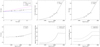 |
Fig. A.1. Model-fitting results for knot B5. |
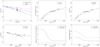 |
Fig. A.2. Model-fitting results for knot K2: Case 1. |
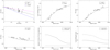 |
Fig. A.3. Model-fitting results for knot K2: Case 2. |
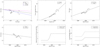 |
Fig. A.4. Model-fitting results for knot K3: Case 1. |
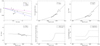 |
Fig. A.5. Model-fitting results for knot K3: Case 2. |
Appendix B: Figures for knots B1, B3, and K1 of jet-B (Figs. B.1–B.4)
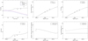 |
Fig. B.1. Model-fitting results for knot B1. |
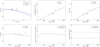 |
Fig. B.2. Model-fitting results for knot B3. |
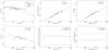 |
Fig. B.3. Model-fitting results for knot K1: Case 1. |
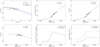 |
Fig. B.4. Model-fitting results for knot K1: Case 2. |
All Tables
Model parameters for the six superluminal knots (B4, B5, K2, K3, K09, and K14) of jet-A.
Model parameters for the seven superluminal components (B1, B2, B3, B6, K1, K10, and K16) of jet-B.
All Figures
|
Fig. 1. Geometry of the precession helical trajectory model. Superluminal knots move along a helical trajectory around the jet axis defined by the function x0(z0) in the plane (X, Z), having an amplitude A(s0) and phase ϕ(s0) defined in the coordinate system (x′, y′, z′). Through transformation among the coordinate systems, the apparent trajectory and the kinematic parameters (bulk Lorentz factor, Doppler factor, apparent velocity, and viewing angle) of a knot can be derived from its spatial trajectory and spatial kinematics by using the formulas given in Sect. 2. |
| In the text | |
|
Fig. 2. Jet-A: Modeled precessing common trajectory distribution (upper panel) and the observed trajectories of knots B5, K09, and K14 for comparison (lower panel). |
| In the text | |
|
Fig. 3. Model fitting results for knot B4. |
| In the text | |
|
Fig. 4. Model fitting results for knot K09: Case 1. |
| In the text | |
|
Fig. 5. Model fitting results for knot K09: Case 2. |
| In the text | |
|
Fig. 6. Model fitting results for knot K14: Case 1. |
| In the text | |
|
Fig. 7. Model fitting results for knot K14: Case 2. |
| In the text | |
|
Fig. 8. Jet B: modeled distribution of precessing common trajectory (upper panel) and the observed trajectories of knots B3, K1, and K10 for comparison. |
| In the text | |
|
Fig. 9. Model fitting results for knot B2. |
| In the text | |
|
Fig. 10. Model fitting results for knot B6. |
| In the text | |
|
Fig. 11. Case 1: Model fitting results for knot K10. |
| In the text | |
|
Fig. 12. Case 2: Model fitting results for knot K10. |
| In the text | |
|
Fig. 13. Similarity of the trajectory sections of knot K16 and B2 between Xn = 0.15 mas and 0.25 mas. This comparison provides a rather important clue, showing that the kinematic behavior of knot K16 should be explained similarly to that of knot B2; an open circle corresponds to K16 and an open triangle corresponds to B2. |
| In the text | |
|
Fig. 14. Model fitting results for knot K16. |
| In the text | |
|
Fig. A.1. Model-fitting results for knot B5. |
| In the text | |
|
Fig. A.2. Model-fitting results for knot K2: Case 1. |
| In the text | |
|
Fig. A.3. Model-fitting results for knot K2: Case 2. |
| In the text | |
|
Fig. A.4. Model-fitting results for knot K3: Case 1. |
| In the text | |
|
Fig. A.5. Model-fitting results for knot K3: Case 2. |
| In the text | |
|
Fig. B.1. Model-fitting results for knot B1. |
| In the text | |
|
Fig. B.2. Model-fitting results for knot B3. |
| In the text | |
|
Fig. B.3. Model-fitting results for knot K1: Case 1. |
| In the text | |
|
Fig. B.4. Model-fitting results for knot K1: Case 2. |
| In the text | |
Current usage metrics show cumulative count of Article Views (full-text article views including HTML views, PDF and ePub downloads, according to the available data) and Abstracts Views on Vision4Press platform.
Data correspond to usage on the plateform after 2015. The current usage metrics is available 48-96 hours after online publication and is updated daily on week days.
Initial download of the metrics may take a while.