| Issue |
A&A
Volume 658, February 2022
|
|
|---|---|---|
| Article Number | A55 | |
| Number of page(s) | 13 | |
| Section | Interstellar and circumstellar matter | |
| DOI | https://doi.org/10.1051/0004-6361/202140495 | |
| Published online | 31 January 2022 | |
Cloud motion and magnetic fields: Four clouds in the Cepheus Flare region
1
Indian Institute of Astrophysics (IIA),
Sarjapur Road, Koramangala,
Bangalore
560034,
India
e-mail: ektasharma.astro@gmail.com
2
Department of Physics and Astrophysics, University of Delhi,
Delhi
110007,
India
3
Max Planck Institute for Astronomy,
Königstuhl 17,
69117,
Heidelberg,
Germany
Received:
4
February
2021
Accepted:
10
August
2021
Context. The Cepheus Flare region consists of a group of dark cloud complexes that are currently active in star formation.
Aims. The aim of this work is to estimate the motions of four clouds, namely L1147/1158, L1172/1174, L1228, and L1251, located at relatively high Galactic latitude (b > 14°) in the Cepheus Flare region. We study the relationship between the motions of the clouds with respect to the magnetic field and the clump orientations with respect to both the magnetic field and the motion.
Methods. We estimated the motions of the molecular clouds using the proper motion and distance estimates of the young stellar objects (YSOs) associated with them using the Gaia EDR3 data. By assuming that the YSOs are associated with the clouds and share the same velocity, the projected directions of motion are estimated for the clouds. We measured the projected geometry of the magnetic field towards the direction of each cloud by combining the Planck polarization measurements.
Results. We estimated a distance of 371 ± 22 pc for L1228 and 340 ± 7 pc for L1251, implying that all four complexes are located at almost the same distance. Assuming that both the clouds and YSOs are kinematically coupled, we estimated the projected direction of motion of the clouds using the proper motions of the YSOs. The directions of motion of all the clouds are offset by ~30° with respect to the ambient magnetic fields, except in L1172/1174 where the offset is ~45°. In L1147/1158, the starless clumps are found to be oriented predominantly parallel to the magnetic fields while prestellar clumps show a random distribution. In L1172/1174, L1228, and L1251, the clumps are oriented randomly with respect to the magnetic field. With respect to the motion of the clouds, there is a marginal trend that the starless clumps are oriented more parallel in L1147/1158 and L1172/1174. In L1228, the major axes of the clumps are oriented more randomly. In L1251, we find a bimodal trend in the case of starless clumps. We do not find any overall specific correlation between the core orientation and the global/local magnetic fields for the clouds in Cepheus. Also, we conclude that the local small-scale dynamics of the cloud with respect to the magnetic field direction could be responsible for the final orientation of the cores.
Key words: ISM: magnetic fields / ISM: structure / polarization / techniques: polarimetric
Note to the reader: The names of authors Ekta Sharma and Sami Dib have been corrected on 4 March 2022, together with the publication of a corrigendum.
© ESO 2022
1 Introduction
The structure of the filamentary molecular clouds could be a consequence of the instabilities in the interstellar medium. The Parker instability is thought to be one of the driving factors in the formation of filamentary molecular clouds (Mouschovias et al. 2009; Heintz et al. 2020). Other possible mechanisms could be the converging flows (e.g., Hennebelle & Pérault 1999; Ballesteros-Paredes et al. 1999; Vázquez-Semadeni et al. 2006; Hennebelle et al. 2007; Inoue & Inutsuka 2009) driven by stellar feedback or turbulence. Stellar feedback processes, such as the expansion of HII regions (Bania & Lyon 1980; Vazquez-Semadeni et al. 1995; Passot et al. 1995), stellar winds, and supernova blast waves (McCray & Kafatos 1987; Gazol-Patiño & Passot 1999; de Avillez 2000; de Avillez & Mac Low 2001; de Avillez & Breitschwerdt 2005; Dib et al. 2006, 2009; Kim et al. 2011; Ntormousi et al. 2011) can generate converging streams of gas that assemble to become molecular clouds, either in the Galactic plane or at relatively high Galactic latitudes. The energy input from supernovae and stellar winds can also eject material vertically upwards (e.g., Spitzer 1990; McKee 1993; Benjamin & Danly 1997) which then flows back into the plane of the disk (vgas < vesc) through the diffuse magnetized interstellar medium (ISM).
Magnetic fields may play a crucial role in the dynamics of cloud motion through the ISM. Using 2D numerical simulations, Mac Low et al. (1994) showed that even a moderate level of magnetic field aligned parallel to the direction of the shock motion can help a cloud stabilize against disruptive instabilities (see also Jones et al. 1996). The magnetic field was found to have an even more dramatic impact when the motion of the cloud was considered transverse to the field lines (Jones et al. 1996). In this case, the field lines at the leading edge of the cloud are stretched, creating a magnetic shield which quenches the disruptive Rayleigh-Taylor and Kelvin-Helmholtz instabilities and thus helps the cloud survive for longer. By varying the magnetic field orientation angle with respect to the cloud motion and also by varying the cloud–background density contrast and the cloud Mach number, Miniati et al. (1999), based on 2D numerical simulations showed that for sufficiently large angles, the magnetic field tension can become significant in the dynamics of the motions of clouds with high density contrast and low Mach number. Gregori et al. (1999, 2000), using 3D numerical simulations of a moderately supersonic cloud motion through a transverse magnetic field, showed that the growth of dynamical instabilities is significantly enhanced by increase in the magnetic pressure at the leading edge of the cloud caused by the effective confinement of the magnetic field lines.
It is interesting to test these theoretical and numerical ideas on the Galactic molecular clouds. The Gould Belt is a distribution of stars and molecular clouds that forms a circular pattern in the sky, and has an inclination of ~ 20° with respectto the Galactic plane (Gould 1879). The minimum and the maximum Galactic latitudes of the Gould Belt are toward the Orion and the Scorpio-Centaurus constellations, respectively. The Cepheus Flare region is considered to be a part of the Gould Belt (e.g., Kirk et al. 2009). This region is identified as having a complex of nebulae that extends 10°–20° out of the plane of the Galactic disk at a Galactic longitude of 110° (Hubble 1934; Lynds 1962; Taylor et al. 1987; Clemens & Barvainis 1988; Dutra & Bica 2002; Dobashi et al. 2005). Five associations of dark clouds are found towards this region, namely L1148/1157, L1172/1174, L1228, L1241, and L1247/1251. There are signs of current star formation in these cloud complexes (e.g., Kirk et al. 2009).
Several shells and loops are identified in the direction of the Cepheus Flare. The Cepheus Flare Shell with its center at the Galactic coordinates l~ 120° and b~ 17° is considered to be an expanding supernova bubble and is located at a distance of ~ 300 pc (Grenier et al. 1989; Olano et al. 2006). Based on a study of the H I distribution in the region of the Cepheus Flare, Heiles (1969) speculated upon the possibility of the presence of two sheets most likely representing an expanding or colliding system at a distance of 300–500 pc. The presence of a giant radio continuum region Loop III centered at l = 124 ± 2°, b = +15.5 ± 3° and extending across 65° (Berkhuijsen 1973) suggests that this system possibly formed as a consequence of multiple supernova explosions. Also, the identification of an H I shell by Hu (1981) at l = 105° and b = +17° suggests that the ISM towards the Cepheus Flare region is far from being static.
Based on a study of the kinematics of the gas in LDN 1157, a star-forming cloud associated with the cloud complex LDN 1147–LDN 1158, Sharma et al. (2020) showed that the southern boundary of the east–west segment was found to show a sinuous feature. Using the proper motion and parallax measurements of YSOs associated with L1147/1158 and L1172/1174, these latter authors suggest that the feature could be produced by the motion of the cloud through the ISM. In this paper, we studied the motion of two more cloud complexes, LDN 1228 (hereafter L1228; Lynds 1962) and LDN 1251 (hereafter L1251; Lynds 1962). These are located in the direction of the Cepheus Flare region (Yonekura et al. 1997) and show signs of active star formation (Kun et al. 2009). Both these clouds are situated towards the east of L1147/1158 and L1172/1174 cloud complexes at an angular separation of ~ 10° (Fig. 1). Using the parallax measurements of the YSOs associated with the clouds from the Gaia EDR3, we find that both L1228 and L1251 are located at similar distances to those of L1147/1158 and L1172/1174 but show different radial velocities (Benson & Myers 1989; Yonekura et al. 1997; Lee et al. 2007). Using the proper motion measurements of the YSO population identified in L1147/1158, L1172/1174, L1228, and L1251, and assuming that both YSOs and the clouds are kinematically coupled, we estimated the motions of the clouds on the plane of the sky.
The plane of the sky component of the magnetic fields towards a molecular cloud are inferred from observations made at optical (e.g., Vrba et al. 1976; Goodman et al. 1990; Alves et al. 2008; Soam et al. 2013, 2015; Pereyra & Magalhães 2004; Franco & Alves 2015; Neha et al. 2016), near-infrared (NIR; e.g., Goodman et al. 1992; Goodman 1995; Chapman et al. 2011; Sugitani et al. 2010; Clemens et al. 2018), far-infrared (FIR; e.g., Clemens et al. 2018; Chuss et al. 2019; Pillai et al. 2020) and submillimeter (submm) wavelengths (Rao et al. 1998; Benoît et al. 2004; Vaillancourt et al. 2007; Dotson et al. 2010; Planck Collaboration Int. XXXV 2016). As the interstellar dust grains align their long axis perpendicular to the magnetic field, the background star light polarization is parallel to the local magnetic field. At FIR and submm wavelengths, thermal dust emission is found to be linearly polarized with the polarization position angles lying perpendicular to the ambient magnetic field orientations (Benoît et al. 2004; Vaillancourt et al. 2007). This provides information on the geometry of the projected magnetic field lines. The magnetic field morphology traced by the polarization measurements made with the Planck are used not only to infer the Galactic magnetic field geometry, but also to place new constraints on the dust grain properties (Planck Collaboration Int. XXI 2015; Planck Collaboration Int. XXXII 2016; Planck Collaboration Int. XXXV 2016; Planck Collaboration Int. XXXVIII 2016). In this study, the plane of the sky component of the magnetic field geometry was inferred for all four clouds using the Planck polarization measurements.
Having information on the motion of the cloud and the magnetic field geometry on the plane of the sky, we studied various relations such as (a) the relative orientation between the projected magnetic field and the direction of motion of the clouds, (b) the relative orientation between the major axis of the core and the orientation of the magnetic fields (both within the cloud and in the inter-cloud region), and (c) the relative orientation between the major axis of the core and the direction of motion of the clouds. This paper is organized in the following manner. We begin with a description of the data used in Sect. 2, followed by a discussion of the YSO population in each cloud, the estimation of the distances of the clouds, and the proper motion values of the YSOs in Sect. 3. The motions of the clouds are discussed with respect to the orientation of the projected magnetic fields, and the orientation of the clumps identified in the clouds are discussed with respect to both the magnetic fields and the direction of motion. We finally conclude our paper with a summary of the results in Sect. 4.
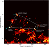 |
Fig. 1 857 GHz Planck image containing the Cepheus Flare region (l ~ 100° − 116° and b ~ 9° − 25°). The four cloud complexes L1147/1158, L1172/1174, L1228, and L1251 studied here are identified and labeled. The arrows drawn in cyan show the direction of motion of the clouds in the sky plane inferred from the proper motion values (Gaia EDR3) of the YSOs associated with the clouds. The median distances of the YSOs estimated using the Gaia EDR3 in this study are also given. |
2 The data
2.1 The Gaia EDR3
The Gaia Early Data Release 3 (EDR3) provides five-parameter astrometric solution, namely positions on the sky (α, δ), parallaxes, and proper motions for more than 1.5 billion sources (Gaia Collaboration 2021). The limiting magnitude is ~ 21 in G-band. Uncertainties in the parallax values are in the range of ~0.02–0.03 mas for sources with G ≤ 15, and around 0.07 mas for sources with G ~ 17 mag. For the sources at the fainter end, with G ~ 20, the uncertainty on parallax is of the order of 0.5 mas (Lindegren et al. 2021). The standard uncertainties in Gaia EDR3 as compared to DR2 have improved on average by a factor of approximately 0.8 for the positions and parallaxes, and 0.5 for the values of proper motions. The uncertainties in the corresponding proper motion values are up to 0.01–0.02 mas yr−1 for G ≤ 15 mag, 0.05 mas yr−1 for G = 17 mag, and 0.4 mas yr−1 for G = 20 mag. The conversion from parallax to distance is known to become nontrivial when the observed parallax is small compared to its uncertainty, especially in cases where σϖ/ϖ ≳ 20% (Bailer-Jones 2015). As a result, by adopting an exponentially decreasing space density prior in distance, Bailer-Jones (2015) estimated distances of about 1.47 billion sources using the Gaia parallax measurements. The distances to the YSOs studied in this work are obtained from the catalog provided by Bailer-Jones et al. (2021) while the proper-motion values are obtained from the Gaia EDR3 (Gaia Collaboration 2021) catalog. We used only those values for which the ratio m/Δm (where m represents either the distances or the proper motions and Δm is the corresponding uncertainties in two quantities) is greater than or equal to 3.
2.2 The Planck 353 GHz polarization measurements
The 353 GHz (850 μm) channel is the highest-frequency polarization-sensitive channel of the Planck. We constructed the geometry of the magnetic fields in the vicinity of L1147/1158, L1172/1174, L1228, and L1251 based on these data. We selected images containing the clouds and smoothed them down to the 8′ resolution to obtain a good signal-to-noise ratio (S/N). As mentioned before, the dust emission is linearly polarized with the electric vector normal to the sky-projected magnetic field, and therefore the polarization position angles were rotated by 90° to infer the projected magnetic field.
2.3 Identification of clumps from the Herschel column density maps
In our analysis, we used the sample of cores identified by Di Francesco et al. (2020) using Getsources on high-resolution column density images of four complexes. The method Getsources is a multi-scale method to filter out emission from monochromatic images. Out of all the sources, we have considered only those sources where the aspect ratio is less than 0.8.
To check the dependency of our analysis on any core-extraction method, we also identified clumps in the column density maps of the four clouds using the Astrodendro algorithm, which is a Python package to identify and characterize hierarchical structures in images and data cubes. The dust column density maps of the four clouds L1147/1158, L1172/1174, L1228, and L1251 were obtained from the Herschel Gould Belt Survey Archive1. A dendrogram is a tree diagram which identifies the hierarchical structures of two- and three-dimensional datasets. The structures start from the local maximum, with the volumes getting bigger when the structures merge with the surroundings with lower flux densities (Rosolowsky et al. 2008). The dendrogram method identifies emission features at successive isocontours in emission maps, which are called leaves, and finds the intensity values at which these features merge with neighbouring structures (branches and trunks). In order to extract the structures, three parameters need to be defined : min_value, min_delta, and min_npix. The parameter min_value is an emission threshold above which all the structures are identified and min_delta is a contour interval that decides the boundary between the distinct structures. The initial threshold and the contour step size are selected as a multiple of σ, the rms of the intensity map. In our analysis, we are interested in the denser regions that are identified as leaves.
In each cloud, the minimum threshold was selected as a multiple of the background column density values, ~0.5–65 × 1021 cm−2. We considered emission-free regions well away from the cloud emission to find the background column density. The other parameter, min_delta, decides whether the main structure is to be identified as an independent entity or is merged with the main structure. After trying a set of choices, we used twice the rms of the emission map to minimize the chance of picking up of noise structure. In order to identify the real structures, we used the condition on the size of the clump according to which the area within each ellipse should be higher than the area within 30 pixels for the high-resolution image. Second, we excluded the clumps where the area of each source is smaller than the area subtended by a beam. Here, we used the Herschel column density map for the source extraction with a beam size of ~18′′. In addition to that, to consider only the elongated clumps, we used only those clumps where the aspect ratio is less than 0.8 (Chen et al. 2020). As we are interested in the orientation of cores embedded within the large clouds, we removed those clumps from our sample that are lying on the edges of the dust column density maps.
3 Results and discussion
3.1 Population of YSOs, distance, and proper motion
The star-forming regions in the Cepheus Flare have been extensively studied by Kirk et al. (2009), Kun et al. (2009), and Yuan et al. (2013). The YSOs used in the present study are taken from the above three works. We obtained Gaia EDR3 data for the three YSO candidates that are located in the direction of the L1147/1158 cloud complex (Kirk et al. 2009). These sources are listed in Table 1. The distance and proper motion values of these three sources associated with the L1147/1158 cloud complex are shown in Fig. 2 using open circles (μα⋆) and triangles (μδ) in blue. The median and the standard deviation values of the distances and μα⋆ and μδ are found to be 333 ±1 pc, 7.764 ± 0.137 masẏr−1, and −1.672 ± 0.108 mas yr−1 respectively.These values are given in Cols. 2–4 of Table 2.
Recently, Saha et al. (2020) studied the YSO candidates in the direction of L1172/1174 based on the Gaia DR2 data. These authors obtained the Gaia DR2 data for a total of 19 known YSOs compiled from Kirk et al. (2009), Kun et al. (2009) and Yuan et al. (2013). The filled circles and triangles in red in Fig. 2 show their results for L1172/1174. The medianand median absolute deviation (MAD), which are more robust against outliers, for the distances μα⋆ and μδ are 333 ± 6 pc, 7.473 ± 0.353 mas yr−1, and −1.400 ± 0.302 mas yr−1, respectively. In Fig. 2, we also draw ellipses with 3 × MAD (darker shade) and 5× MAD (lighter shade) for L1172/1174. Of the 19 sources found towards L1172/1174, three sources are found to fall outside the ellipses drawn with 5 × MAD. These sources are shown using open squares (μα⋆) and inverted triangles (μδ) respectively. Only the sources that fall within the limit of 5 × MAD ellipses are considered for our study because these sources with the significant values of proper motion and distance areconsidered to be a member of the particular complex and the remaining ones are considered as outliers. The three sources identified in the direction of L1147/1158 are also found to fall within the 5 × MAD ellipses obtained for L1172/1174 cloud. These sources are listed in Table 1.
The YSO candidates towards L1228 and L1251 are obtained from the source list provided by Kun et al. (2009). We obtained Gaia EDR3 data for 12 and 13 sources towards L1228 and L1251 respectively. The results are shown in Fig. 3 using the filled circles and triangles in blue (L1228) and red (L1251) respectively. The mean and the MAD values of the distance and the proper motions μα⋆ and μδ obtained for L1147/1158, L1172/1174, L1228, and L1251 complexes are given in Cols. 2–4 of Table 2. Two sources belonging to L1251 are found to fall outside the ellipses drawn with 5 × MAD which are identified using open squares and inverted triangles in red (L1251). The sources that fall within the 5 × MAD ellipses towards L1228 (12) and L1251 (11) respectively are listed in Table 1.
There is evident clustering of the sources associated with each cloud complex. It is also apparent that both L1147/1158 and L1172/1174 are located at similar distances from us even though they are ~2° apart in the sky. This implies that they are spatially ~10 pc apart. L1228, which is located at an angular distance of ~10° away from both L1147/1158 and L1172/1174, is slightly further away at ~371 pc from us. This translates to a spatial separation of ~60 pc. The errors in the distances for two sources in L1228 from Gaia EDR3 are higher as compared to Gaia DR2 measurements. L1251, which is spatially at a separation of ~6° away from L1228, is located at a distance of ~340 pc. This cloud lies close to the complexes L1147/1158 and L1172/1174. L1251 is also at a spatial separation of ~10° away from both L1147/1158 and L1172/1174. In Fig. 4, we show the μα⋆ and μδ values for L1147/1158, L1172/1174 (magenta + gray), L1228 (blue), and L1251 (red). The median values are identified using dotted lines and the ellipses are drawn using 3 × MAD (darker shade) and 5× MAD (lighter shade). The square symbols show the sources that fall outside the 5 × MAD ellipses in Fig. 2 and hence are not considered in this study. In the proper motion domain also, all but one source in L1148/57/72/74 fall within the 5 × MAD ellipses in Fig. 4. There is clear clustering of sources, implying that the YSO candidates associated with the clouds are moving coherently in space.
In earlier studies, L1228 was considered to be a cloud lying closer to us at a distance of ~ 200 pc (e.g., Kun et al. 2008). Kinematically, this cloud also differs from the rest of the clouds belonging to the Cepheus Flare region. At least three centers of star formation were identified towards L1228 (e.g., Kun et al. 2008). Recently, Zucker et al. (2020) estimated distances to the molecular clouds by inferring the distance and extinction to stars lying projected on the clouds using optical and NIR photometry and the Gaia DR2 parallax measurements. Based on the results of these latter authors, the distances provided for the regions enclosed within the Galactic coordinates l ~ 102°–115° and b ~ 14°–21° are found to be in the range of ~330 pc to ~380 pc. This is relatively consistent with the distances estimated for the four molecular clouds presented here using the YSO candidates associated with the cloud, which is the most direct method for estimating distances to molecular clouds.
Thanks to the Gaia mission, we now have parallax and proper motion measurements for over 1 billion stars with unprecedented accuracy. Though the high-resolution spectroscopy of stars can provide the measurements of radial velocity, it is still not possible to obtain such measurements for YSOs as they are typically fainter in magnitude. On the other hand, it is not possible to measure the proper motion of the molecular clouds as they are not point sources. Therefore, by combining the proper motion measurements of the YSOs associated with a particular molecular cloud, and by assuming that both the YSOs and the cloud share the same motion – as such clouds are the birth places of the YSOs –, we can determine the projected direction of motion of that molecular cloud in the plane of the sky. The proper motions of the sources measured by Gaia are in the equatorial system of coordinates. To understand the motion of objects in the Galaxy, we need to transform the proper motion values from the equatorial to the Galactic coordinate system μl⋆ = μl cos b and μb. We transformed the proper motion values using the expression (Poleski 2013)
![\begin{equation*}\left[\begin{array}{c}\mu_{l\star}\\\mu_{\textrm{b}}\end{array}\right]=\frac{1}{\textrm{cos}b}\begin{bmatrix}\text{C}_{1} & \text{C}_{2}\\-\text{C}_{2} & \text{C}_{1}\end{bmatrix}\left[\begin{array}{c}\mu_{\alpha\star}\\\mu_{\delta}\end{array}\right]\end{equation*}](/articles/aa/full_html/2022/02/aa40495-21/aa40495-21-eq1.png) (1)
(1)
where the term cosb =  and the coefficients C1 and C2 are given as
 (2)
(2)
The equatorial coordinates (αG, δG) of the north Galactic pole are taken as 192°.85948 and 27°.12825, respectively (Poleski 2013). The mean values of μl⋆ and μb calculated for the YSO candidates found towards the four cloud complexes are given in Cols. 5 and 6 of Table 2. If we assume that the cloud and the YSO candidates are expected to share similar kinematics as a result of them being born inside the cloud, then the arrows should also represent the motion of the clouds on the plane of the sky. The presence of a reflection nebulosity around a number of these YSO candidates provides evidence of their clear association with the cloud. The plane-of-the-sky component of the direction of motion ( ) calculated using the mean values of μl⋆ and μb are given in Col. 7 of Table 2. The arrows drawn in black in Fig. 5 show the sense of the motion of the sources on the sky plane with respect to the Galactic north increasing to the east.
We also computed the scale height of the complexes above the Galactic plane which is 87 pc for L1147/1158, 79 pc for L1172/1174, 121 pc for L1228, and 83 pc for L1251. All four clouds are lying at a height in the range of 83–121 pc with the furthest being L1228 which is located at a height of ~ 121 pc above the Galactic midplane. These displacements above the Galactic plane are larger compared with the rms Z-dispersion of the clouds located within 1 kpc (~80 pc; Dame et al. 1987; Cox 2005).
Gaia DR3 results of YSOs associated with the L1147/1158, L1172/1174, L1228 and L1251 complexes.
Gaia DR3 distances, proper motion and direction of magnetic field for L1147/1158, L1172/1174, L1228 and L1251 complexes.
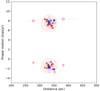 |
Fig. 2 Proper motion vs. distance plot for stars towards L1147/1158 (blue symbols) and L1172/1174 (red symbols). The μα⋆ and μδ are represented using circles and triangles, respectively. Sources listed in Table 1for L1147/1158 and L1172/1174 are shown using blue-filled triangles and circles and red-filled triangles and circles, respectively. The darker and lighter shaded ellipses are drawn using 3 × MAD and 5 × MAD values of the distance and the proper motions, respectively. The sources falling outside of five times the MAD ellipse are shown by squares (μα⋆) and inverted triangles (μδ). |
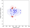 |
Fig. 3 Proper motion vs. distance plot for stars towards L1228 (blue) and L1251 (red). The μα⋆ and μδ are represented using circles and triangles respectively. Sources listed in Table 1 for L1228 and L1251 are shown using blue-filled triangles and circles and red-filled triangles and circles, respectively. The darker and lighter shaded ellipses are drawn using 3 × MAD and 5 × MAD values of the distance and the proper motions, respectively. The sources falling outside of the 5 × MAD ellipse are identified using squares (μα⋆) and inverted triangles (μδ). |
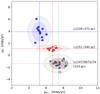 |
Fig. 4 Proper motion values of sources associated with L1147/1158, L1172/1174, L1228 and L1251. The darker and lighter shaded ellipses are drawn using three and five times the median absolute deviation values of the proper motions, respectively.The sources lying outside of the five-times-MAD ellipse are identified using squares symbols. |
3.2 Motion of the cloud complexes with respect to the magnetic field
The plane of the sky magnetic field (Bpos) vectors obtained from the Planck polarization measurements of the region containing all four complexes studied here are shown in Fig. 5. The Bpos vectors are overplotted on the Herschel column density maps. The outermost contour drawn in Fig. 5 corresponds to a column density of 1 × 1021 cm−2. This corresponds to an extinction of AV ≈ 0.5 magnitude determined using the relationship between the column density and the extinction derived by Draine (2003) for the RV = 3.1 extinction law. While the vectors lying within the contour are considered as providing information on the cloud Bpos, the ones lying outside are considered as providing information on the ambient or inter-cloud magnetic field (ICMF) orientation surrounding each cloud. The Bpos vectors lying within ( ) and outside (
 ) of this contour are identified separately using the lines drawn in red + white and white colors respectively.
We find no significant difference between the distributions of  and
and  vectors in L1147/1158, L1228, and L1251, which is very much evident from Fig. 5 also. This implies that the clouds are threaded by the ambient magnetic fields. We find a change in the orientation of the
  and
and  vectors of L1172/1174 which is more prominent as we move to the south and southeast of the cloud. The orientation of the
  and
and  for the clouds is obtained by calculating the median value of all the vectors lying within and outside of the 1 × 1021 cm−2 contour. The values of
  and
and  thus obtained are listed in Col. 10 of Table 2. The
  and the
  determined for the clouds are shown using thick lines in red and cyan in Fig. 5.
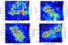 |
Fig. 5 Planck polarization vectors (white) plotted over the column density maps of the clouds produced using the Herschel images. The vectors identified with the red+white vectors correspond to a column density of 1 × 1021 cm−2 which are considered to represent the cloud magnetic field geometry. The arrow drawn in black shows the direction of motion of the clouds. The thick lines drawn in red and cyan are the mean value of the cloud and the background magnetic field orientations, respectively. |
3.2.1 L1147/1158
In L1147/1158, we noted that the cloud complex has strikingly sharp edges to its southern side which is the side facing the Galactic plane. The sharp edges of the southern side of L1147/1158 were also noted by Harjunpaa et al. (1991). The projected direction of motion of L1147/1158 is found to be ~157° with respect to the Galactic north. Our results imply that L1147/L1158 is moving towards the Galactic plane. Interestingly, the sharp edges are developed towards the leading edge of the cloud motion. It is possible that these sharp edges are created as aresult of the interaction of the cloud with the ambient medium through which it is traveling. The projected magnetic field orientations found inside and outside the cloud boundary are found to be at an angle of 183 ± 7° and 186 ± 6°, respectively.The directional offset between the inner and outer magnetic fields is found to be 3°. The projected offsets between the direction of motion of the cloud and the magnetic field orientation inside and outside the cloud boundary are 26° and 29° respectively. Thus the projected motion of the cloud is almost aligned with the ambient magnetic field direction.
3.2.2 L1172/1174
L1172/1174, which seems to be both spatially and kinematically associated with L1147/1158, shows a significant difference in the projected magnetic field orientation especially in its northern and southern regions. The field orientation to the north of L1172/1174 is consistent with the field orientation seen towards L1147/1158. However, it is to the southeastern side of L1172/1174 that the magnetic field orientation becomes more complex. The projected magnetic field orientations inside and outside of the cloud are 208 ± 11° and 196 ± 23° respectively. The directional offset between the inner and outer magnetic fields in L1172/1174 is found to be 12°. The complex magnetic field orientation in the vicinity of the complex is evident from the relatively high dispersion (higher by a factor of two to three compared to the values found towards the other three clouds) found for the field vectors lying outside the cloud. Similar to L1147/L1158, L1172/1174 is also found to be moving towards the Galactic plane. The projected direction of motion of L1172/1174 is estimated to be 151°, which is relatively consistent with the direction of the motion of L1147/1158. Thus, the offsets between the direction of motion of the cloud and the magnetic field orientations found inside and outside of the cloud are 57° and 45° respectively.
3.2.3 L1228
Among the four clouds studied here, L1228 is located at the farthest distance from the Galactic midplane, namely ~121 pc. The direction of motion of L1228 is found to be at an angle of 107° with respect to the Galactic north. The projected orientation of the magnetic field inside and outside of L1228 are found to be 84 ± 7° and 88 ± 10° respectively. We find an offset angle between the inner and outer magnetic fields in L1228 of 4°. The projected direction of motion is at an offset of 23° and 19° with respect to the projected magnetic fields within and outside of the cloud, respectively.
3.2.4 L1251
L1251 is an elongated cloud with a remarkable cometary morphology, which is believed to have been formed as a consequence of its interaction with a supernova bubble as described by Grenier et al. (1989). The elongation of the cloud is in the east–west direction. Two IRAS point sources, associated with molecular outflows, are located in the eastern head region of the cloud while no sign of current star formation was identified in the western region which forms the tail of the cloud (e.g., Kun et al. 2008). Based on the morphology of the cloud produced using the extinction maps generated from the star counts, Balázs et al. (2004) suggested that the cloud resembles a body flying at hypersonic speed across an ambient medium. The projected direction of motion of the cloud is found to be 107°. The projected orientation of the magnetic field inside and outside of L1251 is found to be 79 ± 6° and 81 ± 6°, respectively, and the angular offset between the two fields is 2°. The offset between the projected directions of the motion of the cloud and the inner and the outer magnetic fields are 28° and 26°. It is interesting to note that, at the same time, the cometary morphology of the cloud is oriented parallel to the direction of motion.
The inner and outer magnetic fields in all the four clouds are found to be parallel to each other, suggesting that the inner magnetic fields are inherited from the ambient fields and that the formation of the clouds has not significantly affected the cloud geometries. In a magnetic-field-mediated cloud-formation scenario, the field lines guide the material (Ballesteros-Paredes et al. 1999; Van Loo et al. 2014; Dib et al. 2010) to form the filamentary structures that are expected to be oriented perpendicular to the ambient magnetic fields which then undergo fragmentation to form cores (Polychroni et al. 2013; Könyves et al. 2015; Dib et al. 2020). As the accumulation of the material is helped by the magnetic field lines, the ICMF direction is expected to be preserved deep inside the cores (Li et al. 2009; Hull et al. 2013; Li et al. 2015), leading to a parallel orientation between the ICMF and the core magnetic field.
The magnetic field lines aligned with the cloud motion were studied in 2D numerical simulations by Mac Low et al. (1994). These authors showed that the magnetic fields help to stabilize the cloud against disruptive instabilities. Also using 2D numerical simulations, Miniati et al. (1999) explored the effect of a uniform magnetic field in oblique orientation with respect to a moving interstellar cloud. These latter authors carried out the study for several values of inclination ranging from the aligned case to the transverse case, for several values of Mach number and density contrast parameter, which is the ratio between the cloud and the ambient density. These authors found that for angles of greater than 30°, the magnetic field lines get stretched and tend to wrap around the cloud, amplifying the magnetic field significantly at the expense of the kinetic energy of the cloud.
In all the clouds, the field orientations are smooth and well ordered. In L1148/1157, L1228, and L1251, the offsets between the projected direction of the motion and the projected magnetic fields are ≲30°. No draping of the magnetic fields towards the leading edges of the clouds are seen even in the case of the cometary cloud L1251. However, the offset between the projected direction of the motion and the projected magnetic fields in L1172/1174 is ≳30° and one would expect amplification of the field strength towards its leading edge. Among the four clouds studied here, L1172/1174 is the only cloud that shows an apparent hub–filament structure, forming a massive star, HD200775, and a sparse cluster in the hub. It is interesting to note that in L1172/1174, the deviation in magnetic field as we move from L1147/1158 occurs at the location of the cloud, and then as we move towards the eastern/southeastern sides of L1172/1174, the field geometry becomes complex. It could be possible that a large offset between the cloud motion and the magnetic fields might has helped the cloud to amass material quickly and initiate the formation of the massive star. Whether the modification of the magnetic fields occurred because of the formation of the cloud or the bend in the magnetic field facilitated the formation of the cloud is unclear.
3.3 Magnetic field strength
It is also useful to estimate the magnetic field strength in the four clouds. We used the Davis-Chandrasekhar & Fermi (DCF) (Davis 1951; Chandrasekhar & Fermi 1953) method for the calculation of the plane-of-sky magnetic field strength. The DCF method is given as,
 (3)
(3)
where Δv is the velocity dispersion or the full width at half maximum (FWHM) of the spectral line in units of km s−1,  is the volume density, and Δϕ is the dispersion in polarization angles which is calculated using Stokes parameters as follows:
 (4)
(4)
 (5)
(5)
where ⟨Q⟩ and ⟨U⟩ are the average of the stokes parameters over the selected pixels (Planck Collaboration Int. XIX 2015).
We obtain the velocity dispersion from the most complete CO survey done using the NANTEN telescope, which obtains the spectrum at every one-eighth of a degree across the molecular cloud with a velocity resolution of 0.24 km s−1. Considering the large difference between the beam size of CO and Planck data, we selected only those positions in the cloud where |U|/σU > 3 and |Q|/σQ > 3. This analysis has been adopted from Planck Collaboration Int. XXXV (2016). The number density used in the calculation requires the assumption of a particular cloud geometry for all four clouds, which results in the additional uncertainties. Here, for simplicity, we assume a number density of 100 cm−3 for all the clouds, which is a typical value for the molecular clouds studied here (Draine 2011). The dispersion in the polarization angles (Δϕ) using the stokes parameters at the chosen pixels is 5°–13° and the mean velocity width (FWHM) using 12CO observationsis 2.1–2.7 km s−1. Only those spectra that show a single Gaussian at the selected positions from Stokes parameter maps were chosen. As there is higher dispersion in polarization angles in the case of L1172/1174 over the head part due to the presence of the star HD 200775, we took into account the polarization angles over the tail part of the cloud where the dispersion is due to small-scale variations. The values of the magnetic field strength calculated in the four clouds are 23, 18, 26, and 44 μG for L1147/1158, L1172/1174, L1228, and L1251, respectively. The typical uncertainties in the estimation of magnetic field strength are ~0.5Bpos as found in earlier studies (Crutcher 2004; Planck Collaboration Int. XXXV 2016). This implies that the calculated values of magnetic field strength in all the clouds are comparable within the uncertainty.
3.4 Relative orientations of clumps, magnetic field, and motion of the clouds
The clumps extracted by Di Francesco et al. (2020) in all the four clouds are mostly associated with the filamentary structures which is consistent with the results obtained from the Herschel Gould Belt Survey (André et al. 2010, 2014; Könyves et al. 2010). Theoretically, this association is interpreted as the longitudinal fragmentation of thermally supercritical filaments into cores (e.g., Inutsuka & Miyama 1992, 1997). However, in the presence of turbulence, the filaments cease to become quiescent structures in which perturbations grow slowly. In the case where the clouds are in motion through the ambient ISM, as in the four clouds studied here, they interact with it, generating turbulence in the cloud structure (Mac Low et al. 1994; Jones et al. 1996; Miniati et al. 1999; Gregori et al. 1999, 2000). Under this scenario, we made an attempt to examine the properties of the clumps associated with these clouds with respect to the directions of the  and
and  and the projected direction of their motion,
  . The distribution of the aspect ratio of the identified clumps in each cloud is shown in Fig. 6. The clumps in all the clouds show the whole range of aspect ratios from 0.3 to 0.8. The majority of the cores in all panels (~75%) show aspect ratios of greater than 0.5, which implies that a higher number of sources exhibit a less flattened geometry. As this study is based on projected maps, the lower flattening of cores could also be a consequence of projection effects from the 3D to 2D plane (Chen et al. 2020).
On the basis of the ratio of the mass of the Bonner-Ebert (BE) sphere (Bonnor 1956; Ebert 1955) and the mass of the core (Mcore/MBE), the whole sample of four clouds was classified into prestellar and starless cores by Di Francesco et al. (2020). The cores with a ratio of less than two are considered as starless cores, whereas the ones with a ratio of higher than two are considered as gravitationally bound, termed as candidate prestellar cores, and may collapse to form stars. Assuming the different evolution of the cores in their prestellar and starless stages, we showed their respective distribution separately. The starless cores, being gravitationally unbound, are at an earlier stage of evolution and tend to be more elongated and less spherical in shape compared to the prestellar core evolution. We filtered out the sources with an aspect ratio of less than 0.8 in order to consider only elongated or asymmetric sources. The final sample of prestellar and starless sources for L1147/1158 following this selection is 46 and 75; for L1172/1174 it is 38 and 83; for L1228, it is 54 and 115; for L1251, it is 69 and 89. We notice that a greater number of prestellar cores get filtered out as compared to starless cores, whichimplies that the prestellar cores are more spherical as compared to the starless sample in all four clouds.
We used the position angles of major axis for all the cores extracted from the high-resolution column density map at 18.2′′ resolution (Di Francesco et al. 2020). The offset angles,  ,
,  , and
, and  are calculated. We only show
  here because the values of
  and
and  are comparable within the uncertainties. This shows that the direction of the magnetic field is preserved from cloud to inter-cloud scales. The distributions of
  for all four clouds are shown in Fig. 7 on the left, whereas
  is shown on the right. Towards L1147/1158, for the prestellar cores, the major axis of the clumps is oriented in the range of 30°–60° with respect to the ICMF and the inner magnetic fields. In the case of starless cores, both
  and
and  are found to lie mostly ≤ 30°. The starless cores show a preferred parallel orientation with respect to the magnetic field. In L1172/1174, the orientation of the major axis of the clumps is random compared to that of the cloud magnetic field and the ICMF. Of 38 prestellar cores, the distribution is 11, 14, and 13 clumps, with
  °, 30°
  °, and
  °, respectively. Of the 83 starless clumps identified in L1172/1174, 30, 29, and 24 are present in three ranges implying a uniform distribution. The pattern of
  is also found to be similar to that of
  . In L1228, the offsets
  and
and  show a preferred direction around 40°–60° with a higher number of 20 (37%) sources in this specific range. On the contrary, the distribution is random for the starless cores showing a lack of any preferred orientation. For L1251, there is again a random distribution for starless as well as prestellar cores.
In L1147/1158, the offsets for prestellar cores between the clump major axis and the motion of the cloud,  , are random, whereas in starless cores, a greater number of cores lie ≤ 30°, implying that more clumps are parallel to the projected direction of motion. In L1172/1174, out of 38 prestellar clumps, the offsets show a bimodal distribution with 17 clumps lying at <30° and 14 at >60°. The offsets in starless cores lie mostly at less than 30°, which implies that the clumps are predominantly parallel to the direction of motion. In L1228, the distribution of
  for prestellar cores seems to be more random while for starless cores, there is a preferred orientation with a greater number of clumps lying within the range of 30°–60°. In L1251, out of 69 prestellar clumps, 26 (38%) show the values of
  30° implying that the major axis of the clumps are aligned with the direction of the motion of the cloud. In fact, the cloud also shows a blunt head and a tail which is filamentary and is aligned almost parallel to the direction of motion. It is also important to notice here that the major axis of the majority of the clumps is also aligned along both the filament and the direction of motion of the cloud. Of 80starless clumps, the offset distribution shows a clear bimodal trend where 36 (45%) sources lie below 30° and 27 (33%) sources are oriented at greater than 60°.
As mentioned in Sect. 2.3, to check any dependency on the nature of the source-extraction method, we used Astrodendro to extract the clumps in all four clouds. The parameters used for the extraction are discussed in Sect. 2.3. We derived their properties like the right ascension and the declination of the identified clumps, their effective radius, major and minor axis, and the position angle of the major axis of the clumps ( ). The reference is taken from Galactic north counter-clockwise although the position angle in the Astrodendro is given from the positive x-axis increasing counter-clockwise. We extracted 352 clumps in each of L1147/1158 and 295 in L1172/1174, 437 in L1228, and 345 in the L1251 complex. After applying all the selection criteria on the size and the aspect ratio mentioned in Sect. 2.3, the final number of clumps is 296 in L1147/1158, 259 in L1172/1174, 386 in L1228, and 302 in the L1251 cloud complex. While deriving the sources, we ignored those that are artifacts at the edges in the column density maps. The derived clumps from each cloud are identified in Fig. 5 using ellipses in white.
Figure 8 shows the distribution of the offsets derived using the Astrodendro method for the whole sample without classification. The correlation of the clump orientation with respect to the magnetic field for all four clouds is shown in the upper panel and the clump orientation with respect to the direction of motion is shown in the lower panel. In L1147/1158, the distribution of  and
and  is bimodal although it has preferential alignment of being perpendicular with more clumps at >60°. In L1172/1174, L1228, and L1251, the offsets are random. In L1147/1158, the distribution of the offsets of the clump major axis with respect to the motion of the cloud show more clumps in the range 0°–30°. Similarly, in L1172, the distribution of
  shows a marginal bimodal trend. In L1228, the offsets in the range >60° have the largest number of clumps, suggesting that the clumps tend to be more perpendicular to the direction of motion. In the comet-shaped cloud L1251, the offset distribution shows a bimodal distribution with either parallel or perpendicular orientations. There are 130 clumps lying at <30°, 92 clumps lying in the range 30°
 60°, and 82 clumps having offsets of >60°.
Having derived the histograms of the offsets for the elongated clumps using two different source-extraction methods, we checked for the common sources. By putting a condition between the centroid positions of the clumps as three times the beam width, we checked for the matching sources from both methods. The percentage of common sources for both the methods within this condition has been found to be 70%, 80%, 86%, and 88% for L1147/1158, L1172/1174, L1228, and L1251, respectively. We find that the correlation of the core orientation with the magnetic field and the direction of motion does not follow any systematic trend with either method. The random distribution of the offsets of major axis with respect to magnetic field and the direction of motion in all four clouds suggests that the core orientation depends on the individual cloud magnetization and the local dynamics. It is important to keep in mind that the analyses presented here were carried out on 2D projected maps and therefore the projection from 3D to 2D plane could also affect the measured core morphology. Analyses presented by various authors (Chen et al. 2020; Poidevin et al. 2014) have also suggested that the relative orientation of the cores with respect to the magnetic field is random in nearby star-forming regions like Lupus I, Taurus, Ophiuchus, and Perseus clouds.
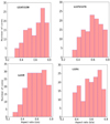 |
Fig. 6 Histogram of the aspect ratios of the clumps extracted from the four clouds. |
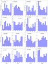 |
Fig. 7 Left (two columns): histograms of the offsets for all four clouds between
|


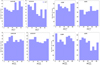 |
Fig. 8 Upper row: histogram of the offsets between the inner or outer magnetic field and the clump orientation. Bottom row: histogram of the offsets between the direction of motion and the clump orientation. |
4 Conclusions
We present results of a study conducted on four molecular cloud complexes situated in the Cepheus Flare region, L1147/1158, L1172/1174,L1228, and L1251. Using the Gaia EDR3 data for the YSOs associated with these clouds we estimate distances of 371 ± 22 pc and 340 ± 7 pc for L1228 and L1251, respectively, implying that all four complexes are located at similar distances from Earth. Using the proper motions of the YSOs with the assumption that the clouds and the YSOs are kinematically coupled, we estimated the projected direction of the motion of the clouds. The clouds are found to be in motion at an offset of ~ 30° with respect to the ambient magnetic fields inferred from the Planck polarization measurements except in the case of L1172/1174 in which the offset is ~ 45°. The inner and outer magnetic field orientations are found to be nearly parallel suggesting that the cloud magnetic fields are inherited from the ICMF.
In L1147/1158, the major axes of the starless clumps are found to be oriented predominantly parallel to both ICMF and cloud magnetic fields while this orientation is around 40° for prestellar cores. In L1172/1174, the major axes of the clumps are found to be aligned more randomly with respect to the field lines for both starless and prestellar clumps. In L1228 and L1251, the offsets between the major axis of the clumps and the field lines are found to be more random for starless clumps, whereas the offsets are overall more around 40°-80° for prestellar clumps. It is possible that the different preferred alignments or the random distribution of the major axis of the cores are related to the local magnetized properties of each cloud.
With respect to the motion of the clouds, there is a marginal trend of the major axis of the prestellar clumps to be more parallel in L1251 and to follow a bimodal distribution for starless clumps. For L1158, starless clumps are oriented closer to parallel but this orientation has a random distribution for prestellar clumps. In L1172/1174, the major axis for starless cores are oriented more randomly whereas for prestellar clouds, major axis follows a roughly bimodal distribution. In L1228, both the starless and prestellar cores show a random distribution in this orientation. The preferred alignment of core orientation with respect to the direction of motion in these clouds suggests that the projected direction of motion could be a regulator of the core dynamics.
Acknowledgements
This research has made use of data from the Herschel Gould Belt survey project (http://gouldbelt-herschel.cea.fr). The HGBS is a Herschel Key Project jointly carried out by SPIRE Specialist Astronomy Group 3 (SAG3), scientists of several institutes in the PACS Consortium (CEA Saclay, INAF-IAPS Rome and INAF-Arcetri, KU Leuven, MPIA Heidelberg), and scientists of the Herschel Science Center (HSC). This work has made use of data from the following sources: (1) European Space Agency (ESA) mission Gaia (https://www.cosmos.esa.int/gaia), processed by the Gaia Data Processing and Analysis Consortium (DPAC, https://www.cosmos.esa.int/web/gaia/dpac/consortium). Funding for the DPAC has been provided by national institutions, in particular the institutions participating in the Gaia Multilateral Agreement; (2) the Planck Legacy Archive (PLA) contains all public products originating from the Planck mission, and we take the opportunity to thank ESA/Planck and the Planck collaboration for the same; (3) the Herschel SPIRE images from Herschel Science Archive (HSA). Herschel is an ESA space observatory with science instruments provided by European-led Principal Investigator consortia and with important participation from NASA. Some of the results in this paper have been derived using the healpy and HEALPix package. We also used data provided by the SkyView which is developed with generous support from the NASA AISR and ADP programs (P.I. Thomas A. McGlynn) under the auspices of the High Energy Astrophysics Science Archive Research Center (HEASARC) at the NASA/GSFC Astrophysics Science Division.
References
- Alves, F. O., Franco, G. A. P., & Girart, J. M. 2008, A&A, 486, L13 [NASA ADS] [CrossRef] [EDP Sciences] [Google Scholar]
- André, P., Men’shchikov, A., Bontemps, S., et al. 2010, A&A, 518, L102 [NASA ADS] [CrossRef] [EDP Sciences] [Google Scholar]
- André, P., Di Francesco, J., Ward-Thompson, D., et al. 2014, Protostars and Planets VI, 27 [Google Scholar]
- Bailer-Jones, C. A. L. 2015, PASP, 127, 994 [Google Scholar]
- Bailer-Jones, C. A. L., Rybizki, J., Fouesneau, M., Demleitner, M., & Andrae, R. 2021, AJ, 161, 147 [Google Scholar]
- Balázs, L. G., Ábrahám, P., Kun, M., Kelemen, J., & Tóth, L. V. 2004, A&A, 425, 133 [NASA ADS] [CrossRef] [EDP Sciences] [Google Scholar]
- Ballesteros-Paredes, J., Hartmann, L., & Vázquez-Semadeni, E. 1999, ApJ, 527, 285 [NASA ADS] [CrossRef] [Google Scholar]
- Bania, T. M., & Lyon, J. G. 1980, ApJ, 239, 173 [NASA ADS] [CrossRef] [Google Scholar]
- Benjamin, R. A., & Danly, L. 1997, ApJ, 481, 764 [NASA ADS] [CrossRef] [Google Scholar]
- Benoît, A., Ade, P., Amblard, A., et al. 2004, A&A, 424, 571 [NASA ADS] [CrossRef] [EDP Sciences] [Google Scholar]
- Benson, P. J., & Myers, P. C. 1989, ApJS, 71, 89 [Google Scholar]
- Berkhuijsen, E. M. 1973, A&A, 24, 143 [NASA ADS] [Google Scholar]
- Bonnor, W. B. 1956, MNRAS, 116, 351 [NASA ADS] [CrossRef] [Google Scholar]
- Chandrasekhar, S., & Fermi, E. 1953, ApJ, 118, 113 [Google Scholar]
- Chapman, N. L., Goldsmith, P. F., Pineda, J. L., et al. 2011, ApJ, 741, 21 [NASA ADS] [CrossRef] [Google Scholar]
- Chen, C.-Y., Behrens, E. A., Washington, J. E., et al. 2020, MNRAS, 494, 1971 [Google Scholar]
- Chuss, D. T., Andersson, B. G., Bally, J., et al. 2019, ApJ, 872, 187 [Google Scholar]
- Clemens, D. P., & Barvainis, R. 1988, ApJS, 68, 257 [Google Scholar]
- Clemens, D. P., El-Batal, A. M., Cerny, C., et al. 2018, ApJ, 867, 79 [CrossRef] [Google Scholar]
- Cox, D. P. 2005, ARA&A, 43, 337 [Google Scholar]
- Crutcher, R. M. 2004, Ap&SS, 292, 225 [NASA ADS] [CrossRef] [Google Scholar]
- Dame, T. M., Ungerechts, H., Cohen, R. S., et al. 1987, ApJ, 322, 706 [NASA ADS] [CrossRef] [Google Scholar]
- Davis, L. 1951, Phys. Rev., 81, 890 [Google Scholar]
- de Avillez, M. A. 2000, MNRAS, 315, 479 [NASA ADS] [CrossRef] [Google Scholar]
- de Avillez, M. A., & Breitschwerdt, D. 2005, A&A, 436, 585 [NASA ADS] [CrossRef] [EDP Sciences] [Google Scholar]
- de Avillez, M. A., & Mac Low, M.-M. 2001, ApJ, 551, L57 [CrossRef] [Google Scholar]
- Dib, S., Bell, E., & Burkert, A. 2006, ApJ, 638, 797 [NASA ADS] [CrossRef] [Google Scholar]
- Dib, S., Walcher, C. J., Heyer, M., Audit, E., & Loinard, L. 2009, MNRAS, 398, 1201 [NASA ADS] [CrossRef] [Google Scholar]
- Dib, S., Hennebelle, P., Pineda, J. E., et al. 2010, ApJ, 723, 425 [NASA ADS] [CrossRef] [Google Scholar]
- Dib, S., Bontemps, S., Schneider, N., et al. 2020, A&A, 642, A177 [NASA ADS] [CrossRef] [EDP Sciences] [Google Scholar]
- Di Francesco, J., Keown, J., Fallscheer, C., et al. 2020, ApJ, 904, 172 [NASA ADS] [CrossRef] [Google Scholar]
- Dobashi, K., Uehara, H., Kandori, R., et al. 2005, PASJ, 57, S1 [Google Scholar]
- Dotson, J. L., Vaillancourt, J. E., Kirby, L., et al. 2010, ApJS, 186, 406 [NASA ADS] [CrossRef] [Google Scholar]
- Draine, B. T. 2003, ARA&A, 41, 241 [NASA ADS] [CrossRef] [Google Scholar]
- Draine, B. T. 2011, Physics of the Interstellar and Intergalactic Medium [Google Scholar]
- Dutra, C. M., & Bica, E. 2002, A&A, 383, 631 [NASA ADS] [CrossRef] [EDP Sciences] [Google Scholar]
- Ebert, R. 1955, ZAp, 37, 217 [Google Scholar]
- Franco, G. A. P., & Alves, F. O. 2015, ApJ, 807, 5 [Google Scholar]
- Gaia Collaboration (Brown, A. G. A., et al.) 2021, A&A, 649, A1 [NASA ADS] [CrossRef] [EDP Sciences] [Google Scholar]
- Gazol-Patiño, A., & Passot, T. 1999, ApJ, 518, 748 [CrossRef] [Google Scholar]
- Goodman, A. A. 1995, in ASP Conf. Ser., 73, From Gas to Stars to Dust, eds. M. R. Haas, J. A. Davidson, & E. F. Erickson [Google Scholar]
- Goodman, A. A., Bastien, P., Myers, P. C., & Menard, F. 1990, ApJ, 359, 363 [NASA ADS] [CrossRef] [Google Scholar]
- Goodman, A. A., Jones, T. J., Lada, E. A., & Myers, P. C. 1992, ApJ, 399, 108 [Google Scholar]
- Gould, B. A. 1879, Result. Observ. Nacional Argent., 1, I [NASA ADS] [Google Scholar]
- Gregori, G., Miniati, F., Ryu, D., & Jones, T. W. 1999, ApJ, 527, L113 [CrossRef] [Google Scholar]
- Gregori, G., Miniati, F., Ryu, D., & Jones, T. W. 2000, ApJ, 543, 775 [NASA ADS] [CrossRef] [Google Scholar]
- Grenier, I. A., Lebrun, F., Arnaud, M., Dame, T. M., & Thaddeus, P. 1989, ApJ, 347, 231 [NASA ADS] [CrossRef] [Google Scholar]
- Harjunpaa, P., Liljestrom, T., & Mattila, K. 1991, A&A, 249, 493 [Google Scholar]
- Heiles, C. 1969, ApJ, 156, 493 [NASA ADS] [CrossRef] [Google Scholar]
- Heintz, E., Bustard, C., & Zweibel, E. G. 2020, ApJ, 891, 157 [NASA ADS] [CrossRef] [Google Scholar]
- Hennebelle, P., & Pérault, M. 1999, A&A, 351, 309 [NASA ADS] [Google Scholar]
- Hennebelle, P., Mac Low, M. M., & Vazquez-Semadeni, E. 2007, ArXiv e-prints, [arXiv:0711.2417] [Google Scholar]
- Hu, E. M. 1981, ApJ, 248, 119 [NASA ADS] [CrossRef] [Google Scholar]
- Hubble, E. 1934, ApJ, 79, 8 [NASA ADS] [CrossRef] [Google Scholar]
- Hull, C. L. H., Plambeck, R. L., Bolatto, A. D., et al. 2013, ApJ, 768, 159 [Google Scholar]
- Inoue, T., & Inutsuka, S.-i. 2009, ApJ, 704, 161 [NASA ADS] [CrossRef] [Google Scholar]
- Inutsuka, S.-I., & Miyama, S. M. 1992, ApJ, 388, 392 [CrossRef] [Google Scholar]
- Inutsuka, S.-i.,& Miyama, S. M. 1997, ApJ, 480, 681 [NASA ADS] [CrossRef] [Google Scholar]
- Jones, T. W., Ryu, D., & Tregillis, I. L. 1996, ApJ, 473, 365 [NASA ADS] [CrossRef] [Google Scholar]
- Kim, C.-G., Kim, W.-T., & Ostriker, E. C. 2011, ApJ, 743, 25 [NASA ADS] [CrossRef] [Google Scholar]
- Kirk, J. M., Ward-Thompson, D., Di Francesco, J., et al. 2009, ApJS, 185, 198 [NASA ADS] [CrossRef] [Google Scholar]
- Könyves, V., André, P., Men’shchikov, A., et al. 2010, A&A, 518, L106 [NASA ADS] [CrossRef] [EDP Sciences] [Google Scholar]
- Könyves, V., André, P., Men’shchikov, A., et al. 2015, A&A, 584, A91 [Google Scholar]
- Kun, M., Kiss, Z. T., & Balog, Z. 2008, Star Forming Regions in Cepheus, ed. B. Reipurth, Vol. 4, 136 [NASA ADS] [Google Scholar]
- Kun, M., Balog, Z., Kenyon, S. J., Mamajek, E. E., & Gutermuth, R. A. 2009, ApJS, 185, 451 [Google Scholar]
- Lee, J.-E., Di Francesco, J., Bourke, T. L., Evans, Neal J., I., & Wu, J. 2007, ApJ, 671, 1748 [NASA ADS] [CrossRef] [Google Scholar]
- Li, H.-b., Dowell, C. D., Goodman, A., Hildebrand, R., & Novak, G. 2009, ApJ, 704, 891 [NASA ADS] [CrossRef] [Google Scholar]
- Li, H.-B., Yuen, K. H., Otto, F., et al. 2015, Nature, 520, 518 [Google Scholar]
- Lindegren, L., Klioner, S. A., Hernández, J., et al. 2021, A&A, 649, A2 [EDP Sciences] [Google Scholar]
- Lynds, B. T. 1962, ApJS, 7, 1 [NASA ADS] [CrossRef] [Google Scholar]
- Mac Low, M.-M., McKee, C. F., Klein, R. I., Stone, J. M., & Norman, M. L. 1994, ApJ, 433, 757 [NASA ADS] [CrossRef] [Google Scholar]
- McCray, R., & Kafatos, M. 1987, ApJ, 317, 190 [NASA ADS] [CrossRef] [Google Scholar]
- McKee, C. F. 1993, in AIP Conf. Ser., 278, Back to the Galaxy, eds. S. S. Holt, & F. Verter, 499 [Google Scholar]
- Miniati, F., Jones, T. W., & Ryu, D. 1999, ApJ, 517, 242 [NASA ADS] [CrossRef] [Google Scholar]
- Mouschovias, T. C., Kunz, M. W., & Christie, D. A. 2009, MNRAS, 397, 14 [NASA ADS] [CrossRef] [Google Scholar]
- Neha, S., Maheswar, G., Soam, A., Lee, C. W., & Tej, A. 2016, A&A, 588, A45 [NASA ADS] [CrossRef] [EDP Sciences] [Google Scholar]
- Ntormousi, E., Burkert, A., Fierlinger, K., & Heitsch, F. 2011, ApJ, 731, 13 [NASA ADS] [CrossRef] [Google Scholar]
- Olano, C. A., Meschin, P. I., & Niemela, V. S. 2006, MNRAS, 369, 867 [NASA ADS] [CrossRef] [Google Scholar]
- Passot, T., Vazquez-Semadeni, E., & Pouquet, A. 1995, ApJ, 455, 536 [NASA ADS] [CrossRef] [Google Scholar]
- Pereyra, A., & Magalhães, A. M. 2004, ApJ, 603, 584 [CrossRef] [Google Scholar]
- Pillai, T. G. S., Clemens, D. P., Reissl, S., et al. 2020, Nat. Astron., 4, 1195 [Google Scholar]
- Planck Collaboration Int. XIX. 2015, A&A 576, A104 [NASA ADS] [CrossRef] [EDP Sciences] [Google Scholar]
- Planck Collaboration Int. XXI. 2015, A&A 576, A106 [NASA ADS] [CrossRef] [EDP Sciences] [Google Scholar]
- Planck Collaboration Int. XXXII. 2016, A&A 586, A135 [NASA ADS] [CrossRef] [EDP Sciences] [Google Scholar]
- Planck Collaboration Int. XXXV. 2016, A&A 586, A138 [NASA ADS] [CrossRef] [EDP Sciences] [Google Scholar]
- Planck Collaboration Int. XXXVIII. 2016, A&A 586, A141 [NASA ADS] [CrossRef] [EDP Sciences] [Google Scholar]
- Poidevin, F., Ade, P. A. R., Angile, F. E., et al. 2014, ApJ, 791, 43 [NASA ADS] [CrossRef] [Google Scholar]
- Poleski, R. 2013, ArXiv e-prints, [arXiv:1306.2945] [Google Scholar]
- Polychroni, D., Schisano, E., Elia, D., et al. 2013, ApJ, 777, L33 [CrossRef] [Google Scholar]
- Rao, R., Crutcher, R. M., Plambeck, R. L., & Wright, M. C. H. 1998, ApJ, 502, L75 [NASA ADS] [CrossRef] [Google Scholar]
- Rosolowsky, E. W., Pineda, J. E., Kauffmann, J., & Goodman, A. A. 2008, ApJ, 679, 1338 [Google Scholar]
- Saha, P., Gopinathan, M., Kamath, U., et al. 2020, MNRAS, 494, 5851 [NASA ADS] [CrossRef] [Google Scholar]
- Sharma, E., Gopinathan, M., Soam, A., et al. 2020, A&A, 639, A133 [NASA ADS] [CrossRef] [EDP Sciences] [Google Scholar]
- Soam, A., Maheswar, G., Bhatt, H. C., Lee, C. W., & Ramaprakash, A. N. 2013, MNRAS, 432, 1502 [NASA ADS] [CrossRef] [Google Scholar]
- Soam, A., Maheswar, G., Lee, C. W., et al. 2015, A&A, 573, A34 [NASA ADS] [CrossRef] [EDP Sciences] [Google Scholar]
- Spitzer, Lyman, J. 1990, ARA&A, 28, 71 [NASA ADS] [CrossRef] [Google Scholar]
- Sugitani, K., Nakamura, F., Tamura, M., et al. 2010, ApJ, 716, 299 [NASA ADS] [CrossRef] [Google Scholar]
- Taylor, D. K., Dickman, R. L., & Scoville, N. Z. 1987, ApJ, 315, 104 [NASA ADS] [CrossRef] [Google Scholar]
- Vaillancourt, J. E., Chuss, D. T., Crutcher, R. M., et al. 2007, SPIE Conf. Ser., 6678, 66780D [NASA ADS] [Google Scholar]
- Van Loo, S., Keto, E., & Zhang, Q. 2014, ApJ, 789, 37 [NASA ADS] [CrossRef] [Google Scholar]
- Vazquez-Semadeni, E., Passot, T., & Pouquet, A. 1995, ApJ, 441, 702 [NASA ADS] [CrossRef] [Google Scholar]
- Vázquez-Semadeni, E., Ryu, D., Passot, T., González, R. F., & Gazol, A. 2006, ApJ, 643, 245 [Google Scholar]
- Vrba, F. J., Strom, S. E., & Strom, K. M. 1976, AJ, 81, 958 [NASA ADS] [CrossRef] [Google Scholar]
- Yonekura, Y., Dobashi, K., Mizuno, A., Ogawa, H., & Fukui, Y. 1997, ApJS, 110, 21 [NASA ADS] [CrossRef] [Google Scholar]
- Yuan, J.-H., Wu, Y., Li, J. Z., Yu, W., & Miller, M. 2013, MNRAS, 429, 954 [NASA ADS] [CrossRef] [Google Scholar]
- Zucker, C., Speagle, J. S., Schlafly, E. F., et al. 2020, A&A, 633, A51 [NASA ADS] [CrossRef] [EDP Sciences] [Google Scholar]
All Tables
Gaia DR3 results of YSOs associated with the L1147/1158, L1172/1174, L1228 and L1251 complexes.
Gaia DR3 distances, proper motion and direction of magnetic field for L1147/1158, L1172/1174, L1228 and L1251 complexes.
All Figures
|
Fig. 1 857 GHz Planck image containing the Cepheus Flare region (l ~ 100° − 116° and b ~ 9° − 25°). The four cloud complexes L1147/1158, L1172/1174, L1228, and L1251 studied here are identified and labeled. The arrows drawn in cyan show the direction of motion of the clouds in the sky plane inferred from the proper motion values (Gaia EDR3) of the YSOs associated with the clouds. The median distances of the YSOs estimated using the Gaia EDR3 in this study are also given. |
| In the text | |
|
Fig. 2 Proper motion vs. distance plot for stars towards L1147/1158 (blue symbols) and L1172/1174 (red symbols). The μα⋆ and μδ are represented using circles and triangles, respectively. Sources listed in Table 1for L1147/1158 and L1172/1174 are shown using blue-filled triangles and circles and red-filled triangles and circles, respectively. The darker and lighter shaded ellipses are drawn using 3 × MAD and 5 × MAD values of the distance and the proper motions, respectively. The sources falling outside of five times the MAD ellipse are shown by squares (μα⋆) and inverted triangles (μδ). |
| In the text | |
|
Fig. 3 Proper motion vs. distance plot for stars towards L1228 (blue) and L1251 (red). The μα⋆ and μδ are represented using circles and triangles respectively. Sources listed in Table 1 for L1228 and L1251 are shown using blue-filled triangles and circles and red-filled triangles and circles, respectively. The darker and lighter shaded ellipses are drawn using 3 × MAD and 5 × MAD values of the distance and the proper motions, respectively. The sources falling outside of the 5 × MAD ellipse are identified using squares (μα⋆) and inverted triangles (μδ). |
| In the text | |
|
Fig. 4 Proper motion values of sources associated with L1147/1158, L1172/1174, L1228 and L1251. The darker and lighter shaded ellipses are drawn using three and five times the median absolute deviation values of the proper motions, respectively.The sources lying outside of the five-times-MAD ellipse are identified using squares symbols. |
| In the text | |
|
Fig. 5 Planck polarization vectors (white) plotted over the column density maps of the clouds produced using the Herschel images. The vectors identified with the red+white vectors correspond to a column density of 1 × 1021 cm−2 which are considered to represent the cloud magnetic field geometry. The arrow drawn in black shows the direction of motion of the clouds. The thick lines drawn in red and cyan are the mean value of the cloud and the background magnetic field orientations, respectively. |
| In the text | |
|
Fig. 6 Histogram of the aspect ratios of the clumps extracted from the four clouds. |
| In the text | |
|
Fig. 7 Left (two columns): histograms of the offsets for all four clouds between
|
| In the text | |
|
Fig. 8 Upper row: histogram of the offsets between the inner or outer magnetic field and the clump orientation. Bottom row: histogram of the offsets between the direction of motion and the clump orientation. |
| In the text | |
Current usage metrics show cumulative count of Article Views (full-text article views including HTML views, PDF and ePub downloads, according to the available data) and Abstracts Views on Vision4Press platform.
Data correspond to usage on the plateform after 2015. The current usage metrics is available 48-96 hours after online publication and is updated daily on week days.
Initial download of the metrics may take a while.