| Issue |
A&A
Volume 645, January 2021
|
|
|---|---|---|
| Article Number | A129 | |
| Number of page(s) | 10 | |
| Section | Interstellar and circumstellar matter | |
| DOI | https://doi.org/10.1051/0004-6361/202039768 | |
| Published online | 29 January 2021 | |
Distances to molecular clouds in the second Galactic quadrant
Purple Mountain Observatory and Key Laboratory of Radio Astronomy, Chinese Academy of Sciences,
10 Yuanhua Road,
Qixia District,
Nanjing 210033,
PR China
e-mail: jiyang@pmo.ac.cn; qzyan@pmo.ac.cn
Received:
27
October
2020
Accepted:
16
December
2020
We present distances to 76 medium-sized molecular clouds and an extra large-scale molecular cloud in the second Galactic quadrant (104. °75 < l < 150. °25 and |b| < 5. °25), 73 of which are accurately measured for the first time. Molecular cloud samples are drawn from l-b-V space (− 95 < VLSR < 25 km s−1) with the density-based spatial clustering of applications with noise algorithm, and distances are measured with the background-eliminated extinction-parallax method using extinctions and Gaia DR2 parallaxes. The range of the measured distances to the 76 molecular clouds is from 211 to 2631 pc, and the extra large-scale molecular cloud appears to be a coherent structure at about 1 kpc, across about 40° (~700 pc) in the Galactic longitude.
Key words: local insterstellar matter / dust, extinction / ISM: clouds / catalogs
© ESO 2021
1 Introduction
As a basic parameter, distance is pivotal to the investigation of the physical properties of molecular clouds (Kennicutt & Evans 2012; Heyer & Dame 2015), as well as their internal structures (Großschedl et al. 2018; Roccatagliata et al. 2020) and distribution in the Milky Way (Reid et al. 2019; Alves et al. 2020). The accuracy of distances to high-mass star-forming regions has improved significantly due to progress in the very long baseline interferometry (VLBI) technique (Xu et al. 2006). For instance, the Bar and Spiral Structure Legacy (BeSSeL) Survey1 (Reid et al. 2014; Zhang et al. 2019; Wu et al. 2019) and the VLBI Exploration of Radio Astrometry (VERA) project2 (Kobayashi et al. 2003; Hirota et al. 2007; Honma et al. 2012; VERA Collaboration 2020) have collectively measured parallaxes of approximately 200 molecular masers toward high-mass star-forming regions with high precision (Reid et al. 2019). With the release of a large amount of stellar parallax and extinction measurements in the Gaia second data release (DR2) catalog (Gaia Collaboration 2016, 2018), distances to many local maser-free molecular clouds can also be accurately determined.
At high Galactic latitudes, the dust environment is relatively simple and measuring distances to molecular clouds with stellar extinction is straightforward. For instance, Zucker et al. (2019, 2020) determined distances to many molecular clouds and star-forming regions at high Galactic latitudes (|b| > 10°), and Yan et al. (2019b) derived distances to ~50 molecular clouds at high Galactic latitudes as well. The systematic error in those distances is about 5%. In addition to accurate distances, large solid angles of molecular clouds at high Galactic latitudes allow us to investigate their three-dimensional (3D) structures and motions. For instance, Großschedl et al. (2018) studied the 3D shape of Orion A and found that it resembles large-scale filaments in the Milky Way. Roccatagliata et al. (2020) studied the Taurus star-forming region with Gaia DR2 parallaxes and proper motions and found that distances to its stellar members are in the range of [130, 160] pc, and they speculated that Taurus B is moving toward Taurus A. Alves et al. (2020) studied the structure of local molecular clouds and found that they show a sinusoidal wave (“Radcliffe wave”) instead of a ring in 3D space.
However, due to the complexity of the interstellar medium, distances to maser-free molecular clouds in the Galactic plane are relatively difficult to measure. In the Galactic plane, the presence of multiple components along the line of sight and the velocity crowding in the inner Galaxy make molecular cloud identification difficult. Consequently, matching dust cloud distances (Green et al. 2019; Chen et al. 2020b,a) to molecular clouds is not straightforward and high-quality spectral images of molecular clouds are needed. In order to deal with molecular cloud distances in the Galactic plane, Yan et al. (2019a) proposed a background-eliminated extinction-parallax (BEEP) method based on the Gaia DR2 data and the Milky Way Imaging Scroll Painting (MWISP) CO survey. This method reveals the extinction jump caused by a molecular cloud using the extinction difference between on- and off-cloud stars. Using this method, Yan et al. (2019a) derived distances to 11 molecular clouds in the third Galactic quadrant (209. °75 < l < 219. °75 and |b| < 5°) and Yan et al. (2020) derived distances to 28 molecular clouds in the first Galactic quadrant (25. °8 < l < 49. °7 and |b| < 5°).
In this work, we examine distances to molecular clouds in the second Galactic quadrant (104. °75 < l < 150. °25 and |b| < 5. °25), which is mapped by the MWISP survey with high sensitivities and moderate angular resolutions (Du et al. 2016, 2017; Sun et al. 2020), including images of three CO isotopolog lines. For the purpose of distance determination, we only use the 12 CO (J = 1 → 0) images to identify molecular clouds with the density-based spatial clustering of applications with noise (DBSCAN) clustering algorithm (Yan et al. 2020), whose distances are subsequently examined with the BEEP method (Yan et al. 2019a).
This paper is organized as follows. The next section (Sect. 2) describes the CO data, the cloud identification algorithm, and the BEEP method. Section 3 presents distances to molecular clouds. Discussions about the molecular cloud distance are presented in Sect. 4, and we summarize our conclusions in Sect. 5.
2 Data and methods
2.1 CO data
The 12CO image of the examined region (104. °75 < l < 150. °25, |b| < 5. °25, and − 95< VLSR < 25 km s−1) is part of the MWISP3 CO survey (Su et al. 2019). The MWISP survey maps the Galactic plane (|b| < 5.25) in the Northern Sky tile by tile (30′ × 30′), and this region in the second Galactic quadrant is complete except for a few tiles at relatively high Galactic latitudes (129° < l < 130° and b = 4. °5). The rms noise of 12 CO is about 0.5 K, and the angular and velocity resolutions are about 49′′ and 0.167 km s−1, respectively.
2.2 Molecular cloud identification
Before measuring distances, we drew molecular cloud samples using the method developed by Yan et al. (2020), which is based on the DBSCAN clustering algorithm4. DBSCAN identifies connected structures in position-position-velocity (PPV) space, paying no attention to the internal structure, the morphology, or the scale of molecular clouds. Without distance information, we initially assumed that close components in PPV space were also close physically, but this assumption can easily be violated. The molecular cloud boundary depends on the sensitivity of observations, and DBSCAN is insensitive to the morphology of molecular clouds. Consequently, the DBSCAN molecular cloud samples contain multiple kinds of shapes, such as cometary structures, Gaussian sources, and filaments. In other words, DBSCAN only searches for separated structures in PPV space.
DBSCAN cloud samples are particularly suitable for distance measurements. Furthermore, splitting large structures in PPV space is meaningless for the BEEP method because there are no nearby off-cloud regions for the interior regions of molecular clouds.
DBSCAN has two parameters, MinPts and ϵ. The ϵ defines the neighborhood of voxels, while MinPts defines core points, which are voxels whose numbers of neighboring voxels (including itself) are at least equal to MinPts. In PPV space, ϵ corresponds to three connectivity types ( ), and, for high values of ϵ, MinPts also needs to be high to avoid including too many noise samples. Yan et al. (2020) found that, for appropriate lower MinPts values, the three connectivity types yield similar cloud samples, so we used connectivity 1 (ϵ = 1) and MinPts 4. The minimum cutoff on thePPV data cubes is 2σ (~1 K).
Due to the low cutoff (2σ), noises are inevitable with connectivity 1 and MinPts 4, and post-selection criteria were applied to remove noise DBSCAB clusters. Here, we followed Yan et al. (2020), using four criteria, two of which are related to sensitivity: (1) the minimum voxel number is 16 and (2) the minimum peak brightness temperature is 5σ. The remaining two criteria are related to resolution: (3) the projection area contains a beam (a compact 2 × 2 region) and (4) the minimum channel number in the velocity axis is 3.
Around −24 km s−1, the data cube contains a bad channel, yielding sample contamination. These fake molecular clouds were removed according to their l-b-v ranges.
2.3 Distance measurement
The procedure of measuring distances using the BEEP method is identical to that in Yan et al. (2020). The BEEP method was developed by Yan et al. (2019a) and is used to measure distances to molecular clouds in the Galactic plane, where the dust environmentis complex. Along the line of sight, stellar extinction picks up variations that are unrelated to the target molecular clouds, hindering accurate distance measurements. To overcome this difficulty, Yan et al. (2019a) proposed using off-cloud stars to trace unrelated extinction variation, which should be subtracted from on-cloud stellar extinction.
The slow irregular increase of off-cloud extinction with respect to the distance is modeled with the isotonic regression (Yan et al. 2019a). Isotonic regression models data with monotonic functions, and monotonically increasing functions are used for the stellar extinction. Essentially, the isotonic regression fits the extinction with multiple step functions to grab the overall variation, and the fitted isotonic regression lines serve as extinction baselines, which are subtracted from the extinction of on-cloud stars. For each molecular cloud, all off-cloud stars collectively yield one extinction baseline, and all on-cloud stars commonly use this baseline.
The BEEP method requires the off-cloud region to be close to the on-cloud region, and both regions need to contain asufficient number of stars to be able to finely reveal the extinction jump. If the off-cloud region is too far, the dust environment of off-cloud stars is dissimilar from that of on-cloud stars and cannot be used for calibration. For large molecular clouds, we manually chose subregions that contained both on- and off-cloud regions (i.e., not all on-cloud stars are used). Molecular cloud edges in the subregions should be relatively sharp in the integrated intensity map. In addition to the closeness, the numbers of on- and off-cloud stars are both required to be sufficiently high to trace the extinction variation reliably due to the large uncertainty in the extinction. For near (<300 pc) or small molecular clouds, there are usually not enough on-cloud stars to reveal distances.
A box region needs to contain both on- and off-cloud stars to measure the molecular cloud distance. The box region is chosen manually, and there are a few useful rules to follow. For a small molecular cloud, a rectangular region that covers the whole molecular cloud and incorporates a comparable surrounding noise region is adequate. For a large molecular cloud, however, multiple medium-sized subregions should be examined, and those with sharply defined boundaries or located at relatively high Galactic latitudes are preferable. If a molecular cloud is both large and nearby (<300 pc), the boxregion should contain the whole molecular cloud so as to use as many on-cloud stars as possible. In Sect. 3, we present three examples of determining box regions in distance measurements, for a large-scale molecular cloud and two molecular clouds with relatively smaller angular areas.
The distance examination procedure starts from the largest molecular clouds. For each molecular cloud, we obtain an integration map in the velocity range [Vcenter − 3ΔV, Vcenter + 3ΔV], where Vcenter is the average radial velocity weighted by the voxel brightness temperature (the first moment) and ΔV is the weighted standard deviation (the second moment). On-cloud stars need to be located within the cloud edge defined by DBSCAN, and, on the contrary, off-cloud stars must be outside the edge. We examined all molecular clouds (1677 in total) with angular areas >0.015 deg2, which is estimated to be the minimum angular area required for distance measurement (Yan et al. 2020).
The CO emission toward on-cloud stars (signal level) needs to be significant to reveal the extinction jump. The signal level used is 4 K km s−1, and the manual choice of signal level is one source of the systematic distance error. The signal level changes the average extinction of background on-cloud stars, thereby changing the distance results; however, the effect of the signal level is insignificant for molecular clouds that show clear extinction jumps. The CO emission toward off-cloud stars (noise level) needs to be low, and the upper limit is 1 K km s−1.
We only kept those molecular clouds that show unique and evident extinction jumps. When AG stars are insufficient, we tried AV measurements (Anders et al. 2019). In order to yield reliable distances, all flags of AV data are required to be 0. To make the results consistent, we calibrated systematic errors in Gaia DR2 following the procedure from Anders et al. (2019). The distance is modeled as a switch point of two Gaussian distributions, from the foreground stellar extinction distribution (a low mean value) to the background stellar extinction (a high mean value), and the model is solved with Markov chain Monte Carlo (MCMC) sampling (Yan et al. 2019b).
The systematic error in the molecular cloud distance is about 5%, which could be larger for distant molecular clouds (>1 kpc). As discussed in Yan et al. (2019b), stellar parallax errors (>10%) could cause systematic shifts (about 10%) in the distance, but this effect is only significant for distant molecular clouds, whose background stars have large relative parallax errors. Other systematic errors arise from the systematic error of Gaia parallaxes, the choice of lower CO emission limits for on-cloud stars, and the choice of the region used to calculate distances. Unknown systematic errors in the stellar extinction are also responsible for the systematic error of molecular cloud distances. By comparing extinction distances of molecular clouds with the VLBI parallax measurements, Yan et al. (2019b) found a systematic error of ~5%. Zucker et al. (2019) estimated a similar value (~5%) for the systematic error, which was attributed to the photometry errors, the stellar models, and the systematic Gaia parallax errors. The effect of the chemical properties of molecular clouds and dust characteristics on the systematic distance error is unknown.
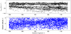 |
Fig. 1 l-V and l-b distributions of the 18 413 molecular clouds identified in the second Galactic quadrant. |
3 Results
3.1 Molecular cloud samples
After removing 88 fake molecular clouds due to a bad channel at about −24 km s−1, DBSCAN identified 18 413 12CO clouds in total. Figure 1 displays the distribution of molecular cloud samples in l-V and l-b spaces. Figure 2 shows the histogram of molecular cloud samples in the projection of l, b, and v spaces.
The Local Arm and the Perseus Arm are well separated by the radial velocity, as shown in panel a of Fig. 2. Molecular cloud samples are roughly homogeneous along the Galactic longitude but show an evident excess above the Galactic plane (b > 0°). This excess is due to the Cepheus Bubble (Patel et al. 1994, 1998) and the warp of the Galactic disk (e.g., Nakanishi & Sofue 2006; Sun et al. 2020).
3.2 The distance catalog
In addition to the largest molecular cloud, which is examined below, 76 (of 1677) molecular clouds have well-determined distances. The nearest cloud is at 211 pc, while the farthest measured distance is 2631 pc. As examples, we display distances to two molecular clouds, G134.7−00.3 (AG) and G112.2−01.5 (AV), in Fig. 3. The angular area of G134.7−00.3 is large, and in order to guarantee a small angular separation between on- and off-cloud stars, we selected a fraction of the cloud; its distance is about 900 pc. G112.2−01.5 is relatively small and isolated, and the numbers of on- and off-cloud stars are significantly lower than those of G134.7−00.3. Distance figures of all molecular clouds are publicly available on the Harvard Dataverse5.
Table A.1 lists distances to 76 molecular clouds. Column (8) is the upper distance cutoff, removing distant background stars that are less useful for the distance determination. The total mass of molecular gas (Col. 9) is derived with the 12 CO-to-H2 mass conversion factor of X = 2.0 × 1020 cm−2  (Bolatto et al. 2013) using the 12CO flux. Column (10) lists the maser-parallax-based distances estimated with the model from Reid et al. (2019).
Figure 4 displays the face-on view of the 76 molecular clouds. Evidently, many molecular clouds gather around 1 kpc, and seven molecular clouds are located in the Perseus Arm, according to the radial velocity (from ~ −60 to ~ −30 km s−1, Sun et al. 2020). G143.7−03.3 is at ~2.1 kpc and possesses the largest scale height (~123 pc).
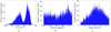 |
Fig. 2 Histograms of the 18 413 molecular clouds in the (a) v, (b) l, and (c) b axes. |
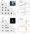 |
Fig. 3 Distances to (a) G134.7−00.3 with AG and (b) G112.2−01.5 with AV. Right-hand plots of both panels: dashed red line is the baseline obtained with off-cloud stars, and the broken horizontal purple line is the extinction variation of on-cloud stars after subtracting the baseline. In the CO image insets, the green and light blue points represent samples of on- and off-cloud stars, respectively. The red line delineates the boundary of molecular clouds, while the green line is the lower cutoff of CO emission toward on-cloud stars. In the CO image insets of panel a, the off-cloud region is selected to be close to the on-cloud region to accurately remove irregular extinction variations of on-cloud stars. The left corner maps are the MCMC sampling results of five parameters: the distance (D), the mean and standard deviation of foreground extinction (μ1 and σ1), and the mean and standard deviation of background extinction (μ2 and σ2). The error ofdistances is the 95% highest posterior densities, about two standard deviations for Gaussian distributions. Further details are available in Yan et al. (2019a). |
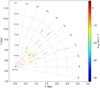 |
Fig. 4 Face-on view of 76 molecular clouds with accurate distance measurements in the second Galactic quadrant. The color represents the radial velocity, and the error bar representing the standard deviation of distance includes the 5% systematic error. The origin of the coordinate is the Galactic center, and the marker sizes are scaled with the mass. |
 |
Fig. 5 Distances to the largest molecular cloud, G125.1+02.6. The edge of the molecular cloud is delineated with the red line. The integrated velocity range is [−22.63, 7.55] km s−1. The distance is in parsecs, and the distances to many molecular clouds around G125.1+02.6 are also displayed. |
3.3 The largest molecular cloud
The angulararea of the largest molecular cloud, G125.1+02.6, is about 107.07 square degrees, which is so large that we had to examine distances to its subregions. Most parts of this cloud are above the Galactic plane, occupying a large range in Galactic longitude, from ~105° to ~145°. The average radial velocity is about − 7.54 km s−1, with a dispersion of 5.03 km s−1.
Distances to G125.1+02.6 are demonstrated in Fig. 5. The background image is the integrated CO intensity map from −22.63 to 7.55 km s−1 (see Fig. 6 for the l-V diagram). Molecular clouds around G125.1+02.6 show similar distance results. Despite the contamination of foreground components at ~350 pc, G125.1+02.6 appears to be a coherent structure at about 1 kpc. The length of G125.1+02.6 is about 700 pc, and, collectively, the mass of G125.1+02.6 is about 1.5 × 10⁷ M⊙.
 |
Fig. 6 l-V diagram of the largest molecular cloud, G125.1+02.6. |
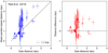 |
Fig. 7 Comparison with maser-parallax-based distances derived from the model in Reid et al. (2019). The error bars represent the standard deviation, and the 5% systematic error is included for Gaia distances. |
4 Discussion
4.1 Comparison with maser-parallax-based distances
In Fig. 7, we compare our distance results with maser-parallax-based distances derived from Reid et al. (2019). As shown in the figure, maser-parallax-based distances are generally compatible with the Gaia distances within errors for local (<1 kpc) molecular clouds. However, for molecular clouds in the Perseus Arm, the maser-parallax-based distance is systematically larger by about 600 pc. Even though Reid et al. (2019) considered the noncircular motions of the Perseus Arm (e.g., Humphreys 1976; Xu et al. 2006; Sun et al. 2020), maser-parallax-based distances may still be systematically larger for many molecular clouds in the Perseus Arm.
4.2 Comparison with previous distance results
The largest cloud contains three well-known star-forming regions, Cep OB3, Sh2-187, and Cam OB1, which are marked in Fig. 5. The parallax distance of 6.7 GHz methanol masers in Cep OB3 is 830 ± 20 pc (Xu et al. 2016), and the photometric distance of Cep OB3 is 850 ± 60 pc (Moreno-Corral et al. 1993); both are consistent with the Gaia DR2 distance, ~800 pc. However, the Gaia DR2 distance to Sh2-187 is about 900 pc, significantly closer than the photometric distance of 1.4 kpc provided by Russeil et al. (2007). The Gaia DR2 distance to Cam OB1 is about 1 kpc, consistent with the photometric distance 975 ± 90 pc (Lyder 2001).
The molecular cloud G134.8+01.4 is associatedwith the W4 H II region (Heyer & Terebey 1998). The driven source of W4 is the open cluster IC 1805, whose distance is 2090.6 pc (Cantat-Gaudin et al. 2018). As demonstrated in Fig. 8, the distance to G134.8+01.4 is  pc, consistent with that of IC 1805 within errors but about 400 pc farther than the distance derived by Zucker et al. (2020) with stellar extinctions and Gaia DR2 parallaxes. In addition to the W4 H II region, distances to two other molecular clouds (see Table A.1), L1265 (G115.6−02.7) and L1320 (G122.4−00.6), are also provided in Zucker et al. (2020). The distance to L1265 given by Zucker et al. (2020) is about 344 pc, which is about 14 pc less than the results of this work. The distance to L1302 of this work is ~1047 pc, which isabout 140 pc farther than that given by Zucker et al. (2020). The results of W4, L1265, and L1302 indicate that the distances from Zucker et al. (2020) may be systematically smaller (~10%) compared to those from our work. This is possibly due to the usage of off-cloud calibration in the BEEP method.
In addition to L1302, G122.4−00.6 also contains a well-known high-mass star-forming region, L1287 (l = 121. °30 and b = 0. °66). The parallax distance of the 6.7 GHz methanol maser emission of L1287 is  pc (Rygl et al. 2010), which is about 100 pc closer than the Gaia extinction distance. Except for the three molecular clouds associated with L1265, L1302, and W4, we did not find accurate distance references for the remaining (73) molecular clouds.
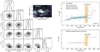 |
Fig. 9 Same as Fig. 3 but for molecular cloud G109.6−01.0, which is the farthest molecular cloud measured. |
4.3 Structure of molecular clouds
Figure 4 shows a clustering of local molecular clouds at about 1 kpc. Taking the largest molecular cloud (Fig. 5) into account, local molecular clouds form a large-scale structure around 1 kpc in the second Galactic quadrant. Evidently, molecular clouds are also present in inter-arm regions.
Due to the limited range in the Galactic longitude, the large-scale structure of molecular clouds is unclear. With the Gaia mission and the MWISP CO survey still ongoing, distances to molecular clouds in the Northern Sky will be measured with a higher completeness, and these measurements are expected to reveal the large-scale structure of local molecular clouds.
4.4 The BEEP method
In this work, we examined 1677 molecular clouds and measured distances to 76 molecular clouds using the BEEP method. The minimum angular area of molecular clouds that have measured distances is 0.02 square degrees. Molecular clouds with smaller angular areas have too few on-cloud stars to finely trace the extinction variation along lines of sight. In addition to the angular size, there are other obstacles that prevented us from measuring distances.
First, distant (>2.5 kpc) and optically thick (>3.5 mag) molecular clouds are not applicable to the BEEP method. In both cases, there are no background stars sufficient for revealing the extinction jump caused by molecular clouds. Figure 9 shows the distance of the farthest molecular cloud, whose background stars are barely sufficient.
Secondly, nearby (<250 pc) molecular clouds usually lack sufficient foreground stars due to the small solid angle, and their distances are usually hard to measure with the BEEP method. Large angular areas are required for those clouds.
Thirdly, molecular clouds with faint CO emission are unable to yield significant extinction jumps. For these molecular clouds, large angular areas and relatively simple dust environments are required. For instance, the BEEP method is still applicable to many diffuse molecular clouds at high Galactic latitudes.
Occasionally, two molecular clouds occupy approximately the same sky region. In this case, the distance usually corresponds to the cloudthat has a higher extinction.
Despite these limitations, the BEEP method measures distances to many local molecular clouds with high accuracy due to its high ability to handle complicated dust environments. With improvements in stellar parallax and extinction precision, the BEEP method is expected to measure distances to many more molecular clouds in the near future.
5 Summary
We have obtained distances to 76 molecular clouds in the second Galactic quadrant, ranging from ~200 to ~2600 pc. We wereable to accurately determine the distances of 73 of these 76 molecular clouds for the first time. In addition, a local large-scale molecular cloud seems to be a coherent structure at about 1 kpc, across about 700 pc in Galactic longitude.
The maser-parallax-based distances to molecular clouds in the Perseus Arm in the second Galactic quadrant is systematically larger than the Gaia DR2 extinction distances by about 600 pc, possibly due to the streaming motion. Extension distances to far (>2.5 kpc) molecular clouds in the Galactic plane are difficult to measure, due to insufficient background stars and the low precision of stellar parallax and extinction data.
Acknowledgements
We would like to show our gratitude to support members of the MWISP group, Zhiwei Chen, Shaobo Zhang, Min Wang, Jixian Sun, and Dengrong Lu, and observation assistants at PMO Qinghai station for their long-term observation efforts. We are also immensely grateful to other member of the MWISP group, Zhibo Jiang, Xuepeng Chen, and Yiping Ao, for their useful discussions. This work was sponsored by the Ministry of Science and Technology (MOST) Grant No. 2017YFA0402701, Key Research Program of Frontier Sciences (CAS) Grant No. QYZDJ-SSW-SLH047, and National Natural Science Foundation of China Grant No. 11773077.
Appendix A Table
Distances to 76 molecular clouds.
References
- Alves, J., Zucker, C., Goodman, A. A., et al. 2020, Nature, 578, 237 [NASA ADS] [CrossRef] [Google Scholar]
- Anders, F., Khalatyan, A., Chiappini, C., et al. 2019, A&A, 628, A94 [NASA ADS] [CrossRef] [EDP Sciences] [Google Scholar]
- Bolatto, A. D., Wolfire, M., & Leroy, A. K. 2013, ARA&A, 51, 207 [Google Scholar]
- Cantat-Gaudin, T., Jordi, C., Vallenari, A., et al. 2018, A&A, 618, A93 [NASA ADS] [CrossRef] [EDP Sciences] [Google Scholar]
- Chen, B., Wang, S., Hou, L., et al. 2020a, MNRAS, 496, 4637 [NASA ADS] [CrossRef] [Google Scholar]
- Chen, B. Q., Li, G. X., Yuan, H. B., et al. 2020b, MNRAS, 493, 351 [NASA ADS] [CrossRef] [Google Scholar]
- Du, X., Xu, Y., Yang, J., et al. 2016, ApJS, 224, 7 [CrossRef] [Google Scholar]
- Du, X., Xu, Y., Yang, J., & Sun, Y. 2017, ApJS, 229, 24 [NASA ADS] [CrossRef] [Google Scholar]
- Gaia Collaboration (Prusti, T., et al.) 2016, A&A, 595, A1 [NASA ADS] [CrossRef] [EDP Sciences] [Google Scholar]
- Gaia Collaboration (Brown, A. G. A., et al.) 2018, A&A, 616, A1 [NASA ADS] [CrossRef] [EDP Sciences] [Google Scholar]
- Green, G. M., Schlafly, E., Zucker, C., Speagle, J. S., & Finkbeiner, D. 2019, ApJ, 887, 93 [NASA ADS] [CrossRef] [Google Scholar]
- Großschedl, J. E., Alves, J., Meingast, S., et al. 2018, A&A, 619, A106 [NASA ADS] [CrossRef] [EDP Sciences] [Google Scholar]
- Heyer, M., & Dame, T. M. 2015, ARA&A, 53, 583 [NASA ADS] [CrossRef] [Google Scholar]
- Heyer, M. H., & Terebey, S. 1998, ApJ, 502, 265 [NASA ADS] [CrossRef] [Google Scholar]
- Hirota, T., Bushimata, T., Choi, Y. K., et al. 2007, PASJ, 59, 897 [NASA ADS] [CrossRef] [Google Scholar]
- Honma, M., Nagayama, T., Ando, K., et al. 2012, PASJ, 64, 136 [NASA ADS] [CrossRef] [Google Scholar]
- Humphreys, R. M. 1976, ApJ, 206, 114 [NASA ADS] [CrossRef] [Google Scholar]
- Kennicutt, R. C., & Evans, N. J. 2012, ARA&A, 50, 531 [NASA ADS] [CrossRef] [Google Scholar]
- Kobayashi, H., Sasao, T., Kawaguchi, N., et al. 2003, ASP Conf. Ser., 306, 367 [NASA ADS] [Google Scholar]
- Lyder, D. A. 2001, AJ, 122, 2634 [NASA ADS] [CrossRef] [Google Scholar]
- Moreno-Corral, M. A., C., C.-K., de La Ra, E., & Wagner, S. 1993, A&A, 273, 619 [Google Scholar]
- Nakanishi, H., & Sofue, Y. 2006, PASJ, 58, 847 [NASA ADS] [Google Scholar]
- Patel, N. A., Heyer, M. H., Goldsmith, P. F., et al. 1994, ASP Conf. Ser., 65, 81 [NASA ADS] [Google Scholar]
- Patel, N. A., Goldsmith, P. F., Heyer, M. H., Snell, R. L., & Pratap, P. 1998, ApJ, 507, 241 [NASA ADS] [CrossRef] [Google Scholar]
- Reid, M. J., Menten, K. M., Brunthaler, A., et al. 2014, ApJ, 783, 130 [Google Scholar]
- Reid, M. J., Menten, K. M., Brunthaler, A., et al. 2019, ApJ, 885, 131 [NASA ADS] [CrossRef] [Google Scholar]
- Roccatagliata, V., Franciosini, E., Sacco, G. G., Randich, S., & Sicilia-Aguilar, A. 2020, A&A, 638, A85 [CrossRef] [EDP Sciences] [Google Scholar]
- Russeil, D., Adami, C., & Georgelin, Y. M. 2007, A&A, 470, 161 [NASA ADS] [CrossRef] [EDP Sciences] [Google Scholar]
- Rygl, K. L. J., Brunthaler, A., Reid, M. J., et al. 2010, A&A, 511, A2 [NASA ADS] [CrossRef] [EDP Sciences] [Google Scholar]
- Su, Y., Yang, J., Zhang, S., et al. 2019, ApJS, 240, 9 [NASA ADS] [CrossRef] [Google Scholar]
- Sun, Y., Yang, J., Xu, Y., et al. 2020, ApJS, 246, 7 [NASA ADS] [CrossRef] [Google Scholar]
- VERA Collaboration (Hirota, T., et al.) 2020, PASJ, 72, 50 [Google Scholar]
- Wu, Y. W., Reid, M. J., Sakai, N., et al. 2019, ApJ, 874, 94 [NASA ADS] [CrossRef] [Google Scholar]
- Xu, Y., Reid, M. J., Zheng, X. W., & Menten, K. M. 2006, Science, 311, 54 [NASA ADS] [CrossRef] [PubMed] [Google Scholar]
- Xu, Y., Reid, M., Dame, T., et al. 2016, Sci. Adv., 2, e1600878 [CrossRef] [Google Scholar]
- Yan, Q.-Z., Yang, J., Sun, Y., Su, Y., & Xu, Y. 2019a, ApJ, 885, 19 [NASA ADS] [CrossRef] [Google Scholar]
- Yan, Q.-Z., Zhang, B., Xu, Y., et al. 2019b, A&A, 624, A6 [NASA ADS] [CrossRef] [EDP Sciences] [Google Scholar]
- Yan, Q.-Z., Yang, J., Su, Y., Sun, Y., & Wang, C. 2020, ApJ, 898, 80 [CrossRef] [Google Scholar]
- Zhang, B., Reid, M. J., Zhang, L., et al. 2019, AJ, 157, 200 [NASA ADS] [CrossRef] [Google Scholar]
- Zucker, C., Speagle, J. S., Schlafly, E. F., et al. 2019, ApJ, 879, 125 [NASA ADS] [CrossRef] [Google Scholar]
- Zucker, C., Speagle, J. S., Schlafly, E. F., et al. 2020, A&A, 633, A51 [CrossRef] [EDP Sciences] [Google Scholar]
All Tables
All Figures
|
Fig. 1 l-V and l-b distributions of the 18 413 molecular clouds identified in the second Galactic quadrant. |
| In the text | |
|
Fig. 2 Histograms of the 18 413 molecular clouds in the (a) v, (b) l, and (c) b axes. |
| In the text | |
|
Fig. 3 Distances to (a) G134.7−00.3 with AG and (b) G112.2−01.5 with AV. Right-hand plots of both panels: dashed red line is the baseline obtained with off-cloud stars, and the broken horizontal purple line is the extinction variation of on-cloud stars after subtracting the baseline. In the CO image insets, the green and light blue points represent samples of on- and off-cloud stars, respectively. The red line delineates the boundary of molecular clouds, while the green line is the lower cutoff of CO emission toward on-cloud stars. In the CO image insets of panel a, the off-cloud region is selected to be close to the on-cloud region to accurately remove irregular extinction variations of on-cloud stars. The left corner maps are the MCMC sampling results of five parameters: the distance (D), the mean and standard deviation of foreground extinction (μ1 and σ1), and the mean and standard deviation of background extinction (μ2 and σ2). The error ofdistances is the 95% highest posterior densities, about two standard deviations for Gaussian distributions. Further details are available in Yan et al. (2019a). |
| In the text | |
|
Fig. 4 Face-on view of 76 molecular clouds with accurate distance measurements in the second Galactic quadrant. The color represents the radial velocity, and the error bar representing the standard deviation of distance includes the 5% systematic error. The origin of the coordinate is the Galactic center, and the marker sizes are scaled with the mass. |
| In the text | |
|
Fig. 5 Distances to the largest molecular cloud, G125.1+02.6. The edge of the molecular cloud is delineated with the red line. The integrated velocity range is [−22.63, 7.55] km s−1. The distance is in parsecs, and the distances to many molecular clouds around G125.1+02.6 are also displayed. |
| In the text | |
|
Fig. 6 l-V diagram of the largest molecular cloud, G125.1+02.6. |
| In the text | |
|
Fig. 7 Comparison with maser-parallax-based distances derived from the model in Reid et al. (2019). The error bars represent the standard deviation, and the 5% systematic error is included for Gaia distances. |
| In the text | |
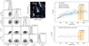 |
Fig. 8 Same as Fig. 3 but for molecular cloud G134.8+01.4, which belongs to the W4 H II region. |
| In the text | |
|
Fig. 9 Same as Fig. 3 but for molecular cloud G109.6−01.0, which is the farthest molecular cloud measured. |
| In the text | |
Current usage metrics show cumulative count of Article Views (full-text article views including HTML views, PDF and ePub downloads, according to the available data) and Abstracts Views on Vision4Press platform.
Data correspond to usage on the plateform after 2015. The current usage metrics is available 48-96 hours after online publication and is updated daily on week days.
Initial download of the metrics may take a while.