| Issue |
A&A
Volume 647, March 2021
First science highlights from SRG/eROSITA
|
|
|---|---|---|
| Article Number | A7 | |
| Number of page(s) | 10 | |
| Section | Interstellar and circumstellar matter | |
| DOI | https://doi.org/10.1051/0004-6361/202039757 | |
| Published online | 26 February 2021 | |
A giant X-ray dust scattering ring discovered with SRG/eROSITA around the black hole transient MAXI J1348–630★
1
Leibniz-Institut für Astrophysik Potsdam (AIP), An der Sternwarte 16,
14482 Potsdam, Germany
e-mail: This email address is being protected from spambots. You need JavaScript enabled to view it.
2
Max-Planck-Institut für extraterrestrische Physik, Gießenbachstraße, 85748 Garching, Germany
3
Dr. Karl Remeis-Sternwarte & Erlangen Centre for Astroparticle Physics, Friedrich-Alexander-Universität Erlangen-Nürnberg, Sternwartstraße 7, 96049 Bamberg, Germany
Received:
25
October
2020
Accepted:
17
December
2020
Abstract
We report the discovery of a giant dust scattering ring around the Black Hole transient MAXI J1348−630 with SRG/eROSITA during its first X-ray all-sky survey. During the discovery observation in February 2020, the ring had an outer diameter of 1.3 deg, growing to 1.6 deg by the time of the second all-sky survey scan in August 2020. This makes the new dust ring by far the largest X-ray scattering ring observed so far. Dust scattering halos, in particular the rings found around transient sources, provide an opportunity to make precise distance measurements towards the original X-ray sources. We combine data from SRG/eROSITA, XMM-Newton, MAXI, and Gaia to measure the geometrical distance of MAXI J1348−630. The Gaia data place the scattering dust at a distance of 2050 pc. Based on the measured time lags and the geometry of the ring we find MAXI J1348−630 at a distance of 3390 pc with a statistical uncertainty of only 1.1% and a systematic uncertainty of 10% caused mainly by the parallax offset of Gaia. This result makes MAXI J1348−630 one of the black hole transients with the most accurately determined distances. The new distance leads to a revised mass estimate for the black hole of 11 ± 2 M⊙. The transition to the soft state during the outburst occurred when the bolometric luminosity of MAXI J1348−630 reached 1.7% of its Eddington luminosity.
Key words: dust, extinction / stars: black holes / stars: distances / stars: individual: MAXI J1648-630 / X-rays: ISM / X-rays: binaries
Based on observations obtained with XMM-Newton, an ESA science mission with instruments and contributions directly funded by ESA Member States and NASA.
© ESO 2021
1 Introduction
Similar to optical light, X-rays from cosmic sources are affected by the interstellar medium in our Galaxy. These effects consist of both photo-electric absorption and dust extinction (Corrales et al. 2016), which is caused by photo absorption and scattering from dust grains, where in contrast to visible light the scattering of X-rays takes place at small angles. The scattered radiation forms a halo around the point source, such that both components of the extinction can often be determined in a single observation. Such observations allow us to draw conclusions about the physical and chemical properties of the interstellar dust (Mauche & Gorenstein 1986; Mathis & Lee 1991; Predehl & Schmitt 1995; Draine 2003; Xiang et al. 2011; Corrales et al. 2017, and references therein).
As the scattered light has to travel a longer distance than the direct light, brightness variations of the central source appear with a delay in the ‘echo’ of the dust scattering halo. This was proposed as early as 1973 as a method to determine the geometrical distance of X-ray sources (Trümper & Schönfelder 1973), but was only realised 27 years later through a Chandra observation of Cyg X-3 (Predehl et al. 2000). As a rule of thumb, the delay of the echo for a source at a distance of 5 kpc, with dust halfway between the source and the observer for sake of simplicity, is a few hours at 1′, some weeks at 10′, and one year at half a degree.
In practice, most X-ray sources show variability on all timescales, and therefore the variability of the halo is very complex as it is the convolution of the impulse response of the halo with the source variability. This makes distance measurements with dust-scattering halos challenging. The best sources for distance measurements with scattering halos are therefore transient X-ray sources, such as X-ray binaries (XRB), soft gamma repeaters (SGRs), or gamma-ray bursts (GRBs), because for these objects, well-defined light echos in the form of distinct rings of X-rays will occur that grow with time. In the case of sources whose distance is known (or very large), such an observation allows a tomography of the dust distribution. Utilising an XMM-Newton observation of expanding rings around GRB031203, Vaughan et al. (2004) were the first to succeed in determining the distance of two dust clouds, at 880 pc and 1.3 kpc. Clark (2004), with a Chandra observation of the X-ray pulsar 4U1538−52, was able to determine both its distance (4.5 kpc) and that of three layers of dust in between (1.3 kpc, 2.56 kpc, and 4.05 pc). Heinz et al. (2015) managed to identify a total of four rings (‘Lord of the Rings’) around Cir X-1. A general consideration of the possibilities of such observations can be found in Corrales et al. (2019). For dust-scattering rings where the distance of either the source or the scattering dust is known from other measurements, the second distance can be calculated geometrically using the ring radius and the time lag of the scattered X-rays. In other cases, both distances have been constrained by modelling the temporal intensity evolution of the expanding rings (e.g. Tiengo et al. 2010). However, this method requires knowledge of the dust scattering cross-section and the results therefore depend on the choice of model for the dust composition and grain-size distribution.
Following the initial report of the detection of a new, bright X-ray transient on 2019 January 26 at 03:16 with MAXI/GSC onboard theInternational Space Station (Yatabe et al. 2019), comprehensive follow-up activities were initiated (e.g. Sanna et al. 2019; Russell et al. 2019a; Lepingwell et al. 2019; Chen et al. 2019a). The monitoring observations of MAXI J1348−630 with MAXI, follow-up X-ray observations with NICER, Swift/XRT, INTEGRAL, and INSIGHT, the identification of an optical counterpart and its spectral shape, and radio observations classified the object as a likely black hole transient (BHT) at αJ2000= 13h48m12.s73, δJ2000 = −63°16′ 26.′′ 8 (Kennea & Negoro 2019) (bII = 309. °26414, lII = -1. °10302). The maximum flux of the source at 1.0 × 10⁻⁷ erg s−1 cm−2 (2–20 keV, ~4 Crab) was reached about 2 weeks after the outburst, followed by a fast decrease of brightness.
Comprehensive analyses of the MAXI and Swift/XRT data assembled during the outburst of the BHT and the following months are presented in Tominaga et al. (2020) and Jana et al. (2020). Hardness intensity diagrams show that the spectral evolution of the source follows the typical track of BHTs and lead to a distance estimate of 3–4 kpc, likely in front of the Scutum-Centaurus arm.
During its first all-sky survey, SRG/eROSITA scanned the sky area of MAXI J1348−630 from 2020 Feb. 18 to 2020 Feb. 24. During routine inspection of the data products generated after daily ground contacts, a large (>1°) and almost perfect circular ring was recognised. A central source was also found coincident with MAXI J1348−630. The structure is thus naturally associated with MAXI J1348−630 and interpreted to be caused by scattered X-rays from the initial burst. Further inspection of the X-ray image revealed further candidate rings (or partial rings) in- and outside of the main ring. An XMM-Newton follow-up observation in Directors Discretionary Time (DDT) was immediately triggered with the aim being to confirm the initial findings, to better qualify the point source contamination of the structure, and to facilitate the spatial and spectral analysis of the rings through improved photon statistics.
In this paper, we present the results of these observations, concentrating on the scattering halo. In contrast to earlier dust-scattering halo measurements, where discovery and follow-up were possible with one of the contemporary wide-angle X-ray cameras onboard, for example, XMM-Newton, Chandra, or Swift/XRT, the case of the dust-scattering echo around MAXI J1348−630 is different. With a size of more than 1° in diameter such a structure can only be discovered through scanning observations similar to those that SRG/eROSITA has been doing since 2019 December 12. With its large field of view of 62′ and its large light-collecting power (comparable to XMM-Newton) the instrument is perfectly suited to making such discoveries, provided the relevant time scales fit with the geometrical setup of the emitter and the scatterer. The remainder of this paper is structured as follows. In Sect. 2 we describe the eROSITA and XMM-Newton observations of MAXI J1348−630. We then discuss the scattering halo, determine the distance to the scatterer and MAXI J1348−630, and perform a spectral analysis of the scattering ring and the post-outburst transient in Sect. 3, and summarise our results in Sect. 4.
2 X-ray observations
2.1 eROSITA observations
Launched on2019 July 13 into an orbit around the L2 point of theEarth–Sun system, the eROSITA instrument onboard the Spectrum-X-Gamma spacecraft (SRG, Sunyaev et al., in prep.) consists of seven X-ray camera assemblies behind seven identical and co-aligned Wolter telescopes; see Merloni et al. (2012) and Predehl et al. (2021) for a description of the instrument and its science goals. Sensitive in the 0.2–8 keV band and with a peak on-axis effective area of over 2000 cm2, since the end of its performance verification phase on 2019 December 13 until the end of 2023, eROSITA will perform the deepest X-ray all-sky survey to date. The eROSITA survey is a slew survey. The telescopes scan along great circles that are approximately perpendicular to the ecliptic, with a rotational axis pointing towards the Earth. This way the whole sky is scanned within 6 months. The rotational period of 4 h together with the 1° field of view means that any patch of sky is seen every 4 h for several eROSITA slews (depending on the ecliptical latitude of the object), andthen again half a year later.
2.1.1 eRASS1
The area around MAXI J1348−630 was scanned 31 times with SRG/eROSITA between MJD 58897.825 and MJD 58903.344. We assume a midpoint of the observations of MJD 58900.583 (2020-02-21 14:00:00 UTC), 391.3 d after the MAXI discovery of the burst. The dust scattering ring, which is rather inconspicuous in unsmoothed event images, was first discovered in smoothed sky maps produced from these data. The vignetted exposure, that is, the equivalent exposure time of an on-axis observation with all seven telescopes, varies between 150 s and 300 s over the area of the scattering ring. We created images in the energy bands 0.2–0.6 keV, 0.6–1.0 keV, and 1.0–2.3 keV. For the purpose of visualisation, the three energy band images were exposure corrected and adaptively smoothed using the eSASS (Brunner et al., in prep.) task erbackmap and combined into a pseudo RGB image (Fig. 1).
From the unsmoothed, exposure-corrected image in the 1.0–2.3 keV band we derived a radial profile of the surface brightness centred at the position of MAXI J1348−630 (Fig. 2). The scattered radiation is detected in an annulus with inner and outer radii of 34′ and 40′, respectively.
2.1.2 eRASS2
The sky area of the scattering ring was covered again during the second eROSITA all-sky survey (eRASS2) with 31 single scans between MJD 59078.597 and MJD 59083.772; the midpoint is MJD 59081.201 (2020-08-20 04:50:00 UTC), or 571.9 days after the MAXI burstdetection. The vignetted exposure of the relevant sky region varies only slightly between 203 and 210 s.
The data were processed in the same way as the eRASS1 data. The dust echo is still visible at the now expected radius, about 1.2 times larger than during the eRASS1 observation but with significantly lower surface brightness (Figs. 1 and 2).
2.2 XMM-Newton
MAXI J1348−630 was observed on 2020 March 10 and 11 by XMM-Newton in Directors Discretionary Time in mosaic mode (observation identifier 0870590101). EPIC/pn, MOS1, and MOS2 were operated in full-frame mode using the medium filter. Eleven EPIC pointings with a total exposure time of 75 ks covered MAXI J1348−630 and almost 60% of the dust ring. The first pointing was exposed for 5.0 ks in MOS and 2.5 ks in pn, the last pointing for 6.2 ks in MOS and 5.9 ks in pn, and the other pointings for 6.6 ks in all instruments. Figure 3 shows the contours of the EPIC/pn and MOS detectors for each sub-pointing. The mosaic-mode data were reduced using the XMM-Newton Science Analysis System (SAS, Gabriel et al. 2004) and split into the sub-pointings by the task emosaic_prep.
To create mosaic images and to perform source detection, they were projected onto common coordinates centred at the mean attitude of all pointings by the task edetect_ stack (Traulsen et al. 2019). Stacked source detection by edetect_stack was used to mask sources in the event lists, from which the radial profile and the spectra were derived. As images with spatially very inhomogeneous background are prone to misinterpretation of background features as extended sources, the task parameters were optimised for point sources. esplinemap in smoothing mode was run with the parameters given by Traulsen et al. (2019), and the source-detection task emldetect was run without extent fitting. In addition to MAXI J1348−630, 280 sources were found. Circular regions with brightness-dependent radius were cut out, a mask including the good source-free regions was generated, and source-excised event lists were created for each pointing and instrument.
Images of all pointings and instruments were created in common coordinates using the task edetect_stack in the five standard XMM-Newton energy bands (1) 0.2–0.5 keV, (2) 0.5–1.0 keV, (3) 1.0–2.0 keV, (4) 2.0–4.5 keV, and (5) 4.5–12.0 keV, and in three energy bands optimised for the flux maximum of the dust ring, derived from the spectra (Sect. 3.4): 0.2–0.8 keV, 0.8–2.2 keV, and 2.2–7.0 keV. The individual images were corrected for background emission and different exposure times and combined into mosaics as follows.
The background of the dust-ring observations is composed of the instrumental background, the local particle background in the orbit, the cosmic X-ray background, and the Galactic components along the line of sight. We model this complex mixture based on source- and ring-free regions in the sub-pointings using the task esplinemap in smoothing mode. For each energy band and instrument, the smoothed background maps of ten sub-pointings were averaged, scaled to the exposure of each sub-pointing, and subtracted from the original images. Pointing 7 was excluded from the averaging because of its high background emission. For EPIC/pn, the out-of-time events were modelled within esplinemap and were also subtracted. The background-subtracted images were exposure-corrected with a combination of exposure maps with and without taking the effects of the mirror vignetting into account. Division of the images by the vignetted exposure maps would give a high weight to the low-exposed outer CCD areas which would appear too bright. Therefore, we used an empirically chosen weighting factor of 0.7 for the vignetted and 0.3 for the unvignetted map. The exposure-corrected images were combined into mosaics. The mosaic image including the dust-ring structure and all sources is shown in Fig. 3. A radial brightness profile with 12 arcsec spacing was derived from the 1− 2 keV mosaic image as described in Sect. 2.1.1 and shown in Fig. 8 (right).
Spectra were generated from the data taken during individual pointings in their genuine coordinates by the task especget using the source-excised event lists. The pn and MOS spectra of MAXI J1348−630 were taken from a circular extraction region with a radius of 20′′ and the background from a nearby half annulus, both centred at the source position. These were grouped to include at least one count in each bin. For the ring spectra, an annular region with an inner radius of 34.5′ and an outer radius of 41.0′ was chosen from the radial profile (Fig. 8). Background spectra were generated from large circular source-free regions outside the ring structure and applied to all sub-pointings for which a similar background level can be expected. The background spectra generated from pointing 1 were used for the ring spectra of pointing 2 and the background of pointing 6 was used for the ring spectra of pointings 6, 8, and 9. In pointings 7, 10, and 11, the background spectra could be used directly. The EPIC/MOS1 and MOS2 spectra of each pointing and their responses were merged by the task epicspeccombine. All spectra were binned to a minimum signal-to-noise ratio (S/N) of 1.0 and were analysed jointly using Xspec version v12.11.1 (heasoft-6.28).
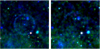 |
Fig. 1 False-colour images of the eRASS1 (18–24 Feb. 2020, left) and eRASS2 (17–22 Aug. 2020, right) observations in the energy bands 0.2−0.6 keV (red), 0.6−1.0 keV (green), 1.0−2.3 keV (blue), adaptively smoothed. The size of the images is 3° × 3°. North is at the top and east to the left. |
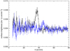 |
Fig. 2 Radial profile of the eRASS1 (black) and eRASS2 (blue) images in the energy band 1.0–2.3 keV with a resolution of 20 arcsec. The scattered emission is detected at radii ~ (34− 40) arcmin in eRASS1 and between ~(40 and 47) arcmin in eRASS2. |
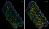 |
Fig. 3 False-colour image of the XMM-Newton mosaic-mode observations in the energy bands 0.2–0.8 keV (red), 0.8–2.2 keV (green), and 2.2–7.0 keV (blue), adaptively smoothed with a two-pixel tophat. The right panel illustrates the 11 sub-pointings with the contours of the three detectors EPIC/pn, MOS1, and MOS2. The position of MAXI J1348−630 is marked near the centre of sub-pointing 04. |
2.3 MAXI
X-ray flux at energies of 2–50 keV from MAXI J1348−630 was detected by MAXI for most of the period within 175 days after the initial discovery on 2019 January 26 (Tominaga et al. 2020). The first outburst peaked 14 days after discovery and after a roughly exponential decay the source disappeared after 104 days. A second, spectrally harder outburst was recorded between days 126 and 175 after discovery. Another re-brightening of MAXI J1348−630 in February 2020 was reported by Shimomukai et al. (2020). The flux levels of this re-brightening were more than two orders of magnitude lower than the primary outburst and therefore this re-brightening is not relevant for the observation of dust scattering.
The dust scattering ring is detected by SRG/eROSITA and XMM-Newton at photon energies of 0.8–2 keV, an energy bandnot covered by MAXI. In order to obtain a light curve in a band which matches the photon energies relevant for the scattering as closely as possible, we downloaded the 2019 MAXI data from the HEASARC mirror. We then used the HEASOFT task mxproduct with standard settings to extract a light curve for MAXI J1348−630 in the energy band 2–3 keV. We removed bad stretches of data during which the line of sight to MAXI J1348−630 was blocked by the Crew Dragon spacecraft docked at the ISS. The remaining data were binned to a resolution of 0.1 days and stretches of missing data were filled by means of interpolation. This light curve (inset in Fig. 4) was used as a reference for the analysis of time lags between the direct flux from MAXI J1348−630 and the scattered X-rays detected by SRG/eROSITA and XMM-Newton.
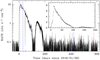 |
Fig. 4 MAXI light curve in the 2–20 keV band. Dashed blue lines indicate XMM-Newton observations (0831000101: 26 ksec, 0831000301: 15 ksec, 0870590101: 77 ksec), dashed red lines eRASS1 and eRASS2 observations. The inset shows the MAXI light curve in the 2–3 keV band in linear representation, binned in 0.1 d intervals and interpolated in periods of missing data. |
3 Analysis and results
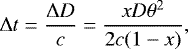
3.1 Scattering geometry
The scattering geometry is illustrated in Fig. 5. It is determined by the distance D to the source, the distance to the scattering layer xD, the opening angle of the scattering ring, θ, and the time-delay Δt between the arrival times of the original signal and the light echo at the observer. The scattered signal will arrive with a time delay of
 (1)
(1)
where the small-angle approximation was used and where ΔD is the additional distance the X-rays travel due to scattering.
Solving Eq. (1) for the angular offset from the source position, θ, results in
 (2)
(2)
For well-defined values of Δt and xD, that is, a sufficiently short burst of radiation and a single layer of dust at distance xD, a scattering ring can be observed.
Observationally, one needs to determine θ and Δt to fix the relative geometry. If either xD or D can be determined independently, the absolute size of the triangle can be derived. Fortunately, this is possible for the light echo around MAXI J1348−630.
3.2 Location of scattering dust
Following Fig. 5 and Eq. (1) the distance D towards the source can be determined from the time lag, Δt, if the distance towards the scattering material xD is known. However, in the real world, this measurement is complicated by the structure of the interstellar medium along the line of sight. The intensity distribution of the halo is therefore given by a convolution of time lags introduced by the dust distribution along the line of sight with the variability of the source.
The circumstances leading to the giant scattering ring around MAXI J1348−630 make this event an ideal opportunity to measure the distance of MAXI J1348−630. The well-defined annular shape of the dust echo is due to the single-peaked burst and also implies the presence of a single, well-defined layer of scattering material. We can confirm this conjecture with a more detailed study of thedust distribution using new Gaia data. Since the Gaia data release DR2 (Arenou et al. 2017) several 3D maps of the interstellar dust extinction in our Milky Way have been published (e.g. Lallement et al. 2019; Chen et al. 2019b). The 3D dust extinction cube published by Lallement et al. (2019) covers a volume of 6 × 6× 0.8 kpc in the solar neighbourhood with 5 pc spatial binning and was derived by combining photometric and astrometric data from Gaia and 2MASS for 27 million stars with Gaia parallax uncertainties of < 20%. We analysed the data cube at the celestial position of MAXI J1348−630 where it extends to a maximum distance of ~3.9 kpc. The most significant regions of extinction are found at distances from the Sun between 1800 and 2200 pc with an integrated AV = 0.9 mag (Fig. 6).
However, the accuracy of the distances in the extinction cube is limited by the fact that the stellar distances were derived by simple inversion of parallaxes, introducing significant bias to the absolute distance scale. In order to eliminate this bias, ancillary data sets with Bayesian estimates of the distances and other stellar parameters have been created. The currently most comprehensive distance set is the Gaia DR2 StarHorse data set (Anders et al. 2019). This catalogue contains 265 million stars with distance, extinction, and other parameters estimated by the StarHorse Bayesian code (Queiroz et al. 2018) using data from Gaia, Pan-STARRS1, 2MASS, and AllWISE. The catalogue is available online1.
In order to determine the dust distribution, we used the subset of the catalogue for the region within 0. °9 of the position of MAXI J1348−630, covering the whole extent of the scattering ring in eRASS1 and eRASS2. We then selected the objects in the area of ‘red clump’ giant stars in the dereddened M0 –(B−R)-plane for our analysis, because these stars are luminous enough to cover the relevant distances and their stellar parameters have accurate estimates. We again consider only stars with relative uncertainties in distance of < 20%. When plotting extinction versus distance for the resulting sample, a steep increase in AV is visible at 2000 pc. It is this region where the scattering ring is formed. In order to determine the distance of the dust causing this extinction, we fit a model for the AV of a simple,homogeneous layer of dust to the data in the distance interval 1500−3000 pc (Fig. 7). The free parameters of the fit are AV,0 (on the near side of the layer), AV,1 (behind the dust), and d0 (distance). The geometrical depth of the dust sheet is well constrained by the X-ray images of the scattering ring and is fixed at 190 pc (see Sect. 3.3 and Table 1). The best-fitting mid-point distance of the dust sheet is at 2047 ± 22pc, and the best-fit extinction values are AV,0 = 0.78 mag and AV,1 = 1.90 mag (see Fig. 7). The resulting distance remains very stable even if the depth of the layer is left free to vary.
 |
Fig. 5 Schematic drawing of the scattering geometry. The distance to the X-ray source is denoted D, and the distance between observer and dust layer is x ⋅ D. The opening angle of the scattering ring is θ, the X-rays are scattered by θsca. |
 |
Fig. 6 Differential extinction on the line of sight towards MAXI J1348−630 extracted from the 3D map compiled by Lallement et al. (2019). |
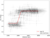 |
Fig. 7 Orthogonal distance regression fit of a homogeneous extinction layer model in the distance–AV plane of the StarHorse data. The depth of the dust layer was fixed to 190 pc. |
3.3 Distance towards MAXI J1348–630
With the distance xD well constrained by the StarHorse data, the distance D to MAXI J1348−630 can be determined using the geometry shown in Fig. 5. However, as discussed above, both the distribution of time lags resulting from the burst light curve (Fig. 4) and the distribution of dust along the line of sight contribute to the width and the radial profile of the ring. For accurate determination of D we therefore modelled the radial profile with the following steps:
- 1.
As for the fit in Fig. 7 we assume a homogeneous dust layer of a certain thickness ddust at a distance xD. The layer was divided into slices of 1 pc depth. For each slice and angle θ we calculated the X-ray flux FX(θ) from the 2–3 keV MAXI light curve (Fig. 4) using the matching time delay Δt at the time of the observation according to Eq. (2).
- 2.
Following Mathis & Lee (1991) and Xiang et al. (2011) the observed brightness distribution as a function of θ from each dust slice at relative distance x is given by
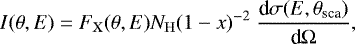 (3)
(3)where FX(E, θ) is the source X-ray flux relevant at angle θ as determined in step 1, NH is the hydrogen column density in the distance slice, and θsca ~ θ∕(1 − x). The scattering cross-section dσ∕dΩ depends on the composition and size distribution of the dust. Draine (2003) gives easy-to-use analytical approximations to the cross-sections for the dust model by Weingartner & Draine (2001) which we adopt here:
![Mathematical equation: \begin{equation*}\frac{\textrm{d}\sigma}{\textrm{d}\Omega} = \frac{\sigma_{\textrm{sca}}}{\pi \theta^2_{\textrm{s,50}}} \frac{1}{\left[1+(\theta_{\textrm{sca}} / \theta_{\textrm{s,50}})^2\right]^2} .\end{equation*}](/articles/aa/full_html/2021/03/aa39757-20/aa39757-20-eq4.png) (4)
(4)We evaluated Eq. (4) at E = 1.5 keV where the characteristic scattering angle is θs,50 = 4′ (Draine 2003). We made no attempt to model the absolute flux of the scattering ring, and therefore in Eqs. (3) and (4) only the dependencies on θ are important here. At a given epoch, the scattering ring covers a relatively small range of angles θ, and therefore the exact function of dσ(θsca)∕dΩ only marginally changes the model profile I(θ). Hence the choice of the model on dust composition and grain size distribution has only negligible influence on our results.
- 3.
The ring profiles from each distance slice were added and the total flux normalised to the observed flux. The result is a model profile for the parameter pair ddust (depth of the dust layer) and D (source distance). To find the best-fitting values for the parameters D and ddust, we calculated the profiles for a grid of D and ddust values and then determined the χ2-values for each resulting profile with respect to the measured profiles from eRASS1 and XMM-Newton. As the X-ray images constrain the depth of the dust layer better than the Gaia data, we re-iterated fitting xD to the StarHorse data with the ddust values derived from X-rays. The parameter space covered in the final run was 140 pc < ddust < 220 pc, 3280 pc < ddust < 3480 pc for the eRASS1 profile and 175 pc < ddust < 205 pc, 3350 pc < ddust < 3440 pc for the XMM-Newton profile.
The fit results for both the eRASS1 and XMM-Newton observations are presented in Table 1 and Fig. 8. It should be noted that using the dust distribution given by the extinction cube by Lallement et al. (2019) (Fig. 6) in the model results in a ring profile which is much broader and more structured than the observed profile, and therefore we conclude that our model assumption of a simple homogeneous layer is a better approximation to the actual distance distribution.
The distance ratio x between the scattering dust and MAXI J1348−630 can be measured with remarkable precision: 0.25% for the XMM-Newton observation and 0.7% for eRASS1. For the XMM-Newton data, the total statistical uncertainties (1.1%) are dominated by the errors in the distance towards the dust layer.
The absolute accuracy of the distance essentially depends on the systematic parallax uncertainties in the Gaia DR2 catalogue, which are still under investigation. Analysis of QSO parallaxes revealed a global negative parallax zero-point but also spatial variations (Lindegren et al. 2018). A systematic uncertainty of ~ 0.05 mas has to been taken into account in the absolute accuracy of distances. In our case this amounts to a 10% absolute accuracy of the measurement to the scattering dust at 2 kpc, and hence the same relative accuracy for the distance towards MAXI J1348−630. The same level of uncertainty has also been adopted by Zucker et al. (2020) for distances of molecular clouds in the 2 kpc range based on Gaia data. However, as the statistical precision of the measurement with respect to the Gaia distance frame is much better, improvements of the absolute Gaia distances in future data releases will directly lead to a higher accuracy of the MAXI J1348−630 distance.
Results of distance measurements.
 |
Fig. 8 Left: background-subtracted eRASS1 ring profile (1.0–2.3 keV) with best-fit model (red line, D = 3390 pc, ddust = 180 pc). Right: background-subtracted XMM EPIC ring profile (1.0–2.0 keV) with best-fit model (red line, D = 3395 pc, ddust = 190 pc). |
3.4 X-ray spectral analysis of the dust-scattering ring
The XMM-Newton EPIC spectra of the dust ring were binned to reach S/Ns of at least 1.0 per bin in the energy range between 0.7 and 2.2 keV in the individual pointings. We fitted them jointly with an absorbed power-law using the absorption model and abundances of Wilms et al. (2000). A multiplicative factor accounted for the different extraction regions and fluxes of the spectra (Xspec model const*tbabs(powerlaw)). The best fit ( for 1 258 degrees of freedom) resulted in
 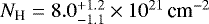 and a power-law index of γ = 4.2 ± 0.4. This NH is consistent with the values obtained for MAXI J1348−630 from other missions. Tominaga et al. (2020) modelled the MAXI spectrum during the high/soft state with a disk black-body model and upscattering at higher energies (tbabs * simpl * diskbb). The resulting disk temperatures at the innermost radius kTRin are in the range 0.6–0.75 keV. In the energy range contributing to the dust scattering ring such a disk black body can be approximated by a power-law with γ ~ 2. When taking into accountthe modification of the incident spectrum by the energy dependence of the scattering cross-section, which is approximately E−2, an absorbed power law with γ ~ 4 can be expected for the ring spectrum. Fixing the power-law index at γ = 4.0, the absorption is better constrained to 7.5 ± 0.4 × 1021 cm−2. To investigate the spatial dependence of the absorption terms, we employ two independent values for the northern and southern parts of the dust ring, coupling pointings 2, 10, and 11 in the north and 6, 7, and 8 in the south. For the fixed power-law index of 4.0, we measure NH,North = 8.7 ± 0.7 × 1021 cm−2 in the northern part of the ring and NH,South = 6.8 ± 0.5 × 1021 cm−2 in the southern part. Figure 9 shows example spectra of a northern and a southern pointing and Table 2 the full list of model parameters.
For both the eRASS1 and eRASS2 observations, event files from the latest eSASS pipeline version (c946) were used to extract spectra of the ring area using the srctool task. For the eRASS1 data, an annulus around the position of MAXI J1348−630 with radii R1 = 34.4 arcmin, R2 = 40.6 arcmin was used to extract the source events. For eRASS2 events in the annulus between R1 = 41.8 arcmin, R2 = 49.3 arcmin were extracted. In both cases, the background was extracted from annuli larger than the source annuli, and intervening sources were excised fromthe source and background regions. Given the limited S/N in the eRASS2 spectrum, we do not expect to measure a spectral index or NH significantly different from eRASS1. Therefore, we only fit this spectrum together with the eRASS1 spectrum and tie the γ and NH parameters, leaving only the normalisations free to vary independently. The resulting model parameters are compiled in Table 3. The spectral indices and absorbing column densities are in line with the XMM-Newton measurements. When fixing NH at the value measured for MAXI J1348−630 (Tominaga et al. 2020), 8.6 × 1021 cm−2, the best-fit photon index is ~ 4.0, as expected for an incident spectrum with γ ~ 2. When fitting both the eRASS1 and eRASS2spectra with fixed NH = 8.6 × 1021 cm−2 and γ = 4.0, the resulting 0.5–2.0 keV fluxes are 5.32 ± 0.27 × 10⁻¹² erg cm−2 s−1 (eRASS1) and 1.57 ± 0.27 × 10⁻¹² erg cm−2 s−1. With 3.4 ± 0.61(1σ) the eRASS1∕eRASS2 flux ratio is somewhat higher than the factor  expected due to the increasing scattering angles and the θ−4 function of the Draine (2003) cross-sections. This might be an indication of a decrease in the scattering cross-sections steeper than ~θ−4. On the other hand one has to consider the large linear size of the ring with a diameter of ~ 50 pc during the time of the eRASS2 observations. Given the azimuthal brightness variations visible in Fig. 3, variations in the dust distribution may also contribute to the observed flux ratio.
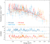 |
Fig. 9 XMM-Newton ring spectra taken by EPIC/pn and MOS in the northern pointing 2 (blue crosses) and the southern pointing 6 (red diamonds) with an absorbed power-law model. The data have been binned to a signal-to-noise ratio of at least 2 for clarity. The residuals (data−model)/error are shown separately in the lower panels. |
Parameters of the fits to XMM-Newton EPIC ring spectra with absorbed power-law models(*), all performed with χ2 fit statistics.
Parameters of the spectral fits to the dust scattering rings in eRASS1 and eRASS2.
3.5 X-ray spectral analysis of MAXI J1348–630 in the post-outburst phase
3.5.1 eRASS1 and eRASS2
In the eRASS1 image, MAXI J1348−630 was clearly detected andwe extracted 95 net counts (0.18 cts s−1) in a circular area with 0.5 arcmin radius. The spectrum was fitted in Xspec with an absorbed power law (tbabs*powl). As the absorbing column density is poorly constrained, it was again fixed to NH= 8.6 × 1021 cm−2. The best-fit spectral index in this case is 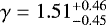 , and the resulting 0.5–2.0 keV flux is (3.04 ± 0.85) × 10−13 erg cm−2 s−1. MAXI J1348−630 was not detected during the eRASS2 observation; the upper limit flux between 0.5 and 2.0 keV is 3 × 10⁻¹⁴ erg cm−2 s−1.
3.5.2 XMM-Newton
MAXI J1348−630 was faint at the time of the XMM-Newton observation with a mean count rate of about 0.005 cts s−1. The EPIC spectra were fitted with an absorbed power law and W statistic (cstat in Xspec), resulting in a poorly constrained 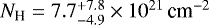 and a power-law index of
  . From the fit to the EPIC/pn spectrum, we derive an absorbed 0.5–2.0 keV flux of
 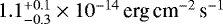 , roughly a factor of ten lower than during eRASS1 just three weeks before the XMM-Newton data were obtained. Fixing column density and power-law index at the eRASS1-derived values, we obtain a flux of
  in the same band.
4 Discussion and conclusion
Since the first hypotheses of dust scattering halos were formulated and after their first successful discovery, almost three decades later, X-ray scattering on interstellar dust has become an established method of determining distances. The method works particularly well when the X-ray source shows bursts, because then instead of a uniform halo, expanding rings can usually be observed. The ambiguity between the distance of the source and the position of the dust can be resolved if one of the two quantities is known. If the source distance can be assumed to be infinite, as in the case of GRBs, the distance between the interstellar dust layers can be determined.
MAXI J1348−630 presents an ideal case for such studies, because the only layer of dust in between is already precisely known based on Gaia measurements, and so that we were able to measure the distance of the X-ray source itself. The distance of 3390 pc has very low statistical uncertainty (1.1%) with respect to the Gaia distance frame, and the absolute accuracy is limited by systematic errors on the Gaia parallaxes which amount to an uncertainty of 10%. This makes the distance to MAXI J1348−630 one of the most accurately determined distances to a black hole binary, which were typically measured with very long baseline interferometry with typical statistical uncertainties on the order of 5–10%. Examples include Cyg X-1, with  kpc (Reid et al. 2011); the systematic uncertainty on this position is large, given its Gaia DR2 distance of
  kpc (Gandhi et al. 2019), which makes it consistent with newer VLBI data (Miller-Jones et al. 2021). A distance to Cyg X-1 has also been calculated by the analysis of its dust-scattering halo by Xiang et al. (2011), who arrive at a distance in the interval 1.72−1.90 kpc.
Our distance improves upon the earlier distance estimates for MAXI J1348−630, which were based on distance indicators that were not well calibrated, such as the transition luminosity between the hard and the soft state. Assuming that this luminosity is between 1 and 4% of the Eddington luminosity (Nowak 1995; Maccarone 2003; Vahdat Motlagh et al. 2019, and references therein), Jana et al. (2020) estimate the distance of MAXI J1348−630 to 5–10 kpc, consistent with the distance estimate based on the dereddened, AV = 2.4, optical magnitude and the position of the object in the optical–X-ray luminosity diagram, which yields D = 3–8 kpc (Russell et al. 2019b). Using the same ansatz, Tominaga et al. (2020) estimate the distance to MAXI J1348−630 to 4-8 kpc. However, noting that with NH ~ 8.6 × 1021 cm−2 the measured X-ray absorption column is significantly lower than the integrated 21 cm interstellar column density (NH ~ (1.45…1.53) × 1022 cm−2, HI4PI Collaboration 2016), Tominaga et al. argue that MAXI J1348−630 must be in front of the Scutum-Centaurus arm (consistent with our result), and then argue for a most likely distance of 3.8 kpc.
Using the MAXI monitoring, Tominaga et al. (2020) used the measured evolution of the inner radius of the accretion disk during the soft state to estimate the mass of the black hole (e.g. Steiner et al. 2010, and references therein). With our improved distance, we can revise their inner disk radius measurements to Rin = 97 ± 13 km (including a systematic error of 10%), leading to a revised estimate of the black hole mass of
 (5)
(5)
compared to the earlier estimate of 13 ± 2 M⊙ (Tominaga et al. 2020). The transition to the soft state, which MAXI measured at a bolometric flux of ~ 1.7 × 10⁻⁸ erg s−1 cm−2 therefore occurred at a luminosity of 1.7% of the Eddington luminosity. With our revised distance and mass, the peak flux of 1.0 × 10⁻⁷ erg s−1 cm−2 given by Tominaga et al. (2020) corresponds to 10% of the Eddington luminosity.
The distance measurement places MAXI J1348−630 at a position between the Sagittarius and Scutum-Centaurus spiral arms of the Milky Way. Figure 10 shows that MAXI J1348−630 is located in an area of relatively low stellar density. With our distance modulus, μ = 12, AV = 2.4, and the quiescence brightness, r′ = 20.69 (Baglio et al. 2020), we derive an absolute magnitude of Mr = 6.24, which is consistent with a main sequence K-type donor star. Both the late-type secondary and the location of the object suggest a relatively old age for the system.
The discovery of this giant scattering ring demonstrates the power of the SRG/eROSITA surveys for this type of science, with their unlimited field of view and six-month observing cadence. With the incidence of new black hole transients being about one per year and the outburst activity of other powerful X-ray sources in our galaxy, we expect further discoveries of dust scattering halos and rings during the 4 years of the survey and significant insights into the physics of both the transient sources and the interstellar medium.
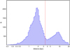 |
Fig. 10 Distance of MAXI J1348−630 (red) compared to the distribution of distances in the Gaia StarHorse data within 0.9 deg from the LOS. |
Acknowledgements
We would like to thank the referee for useful suggestions which helped to improve the presentation of this paper. We thank Friedrich Anders for the useful discussion on the Gaia StarHorse data set and the absolute accuracy of the Gaia parallaxes. This work is based on data from eROSITA, the primary instrument aboard SRG, a joint Russian-German science mission supported by the Russian Space Agency (Roskosmos), in the interests of the Russian Academy of Sciences represented by its Space Research Institute (IKI), and the Deutsches Zentrum für Luft- und Raumfahrt (DLR). The SRG spacecraft was built by Lavochkin Association (NPOL) and its subcontractors, and is operated by NPOL with support from the Max Planck Institute for Extraterrestrial Physics (MPE). The development and construction of the eROSITA X-ray instrument was led by MPE, with contributions from the Dr. Karl Remeis-Observatory Bamberg & ECAP (FAU Erlangen-Nuernberg), the University of Hamburg Observatory, the Leibniz Institute for Astrophysics Potsdam (AIP), and the Institute for Astronomy and Astrophysics of the University of Tübingen, with the support of DLR and the Max Planck Society. The Argelander Institute for Astronomy of the University of Bonn and the Ludwig Maximilians Universität München also participatedin the science preparation for eROSITA. The eROSITA data shown here were processed using the eSASS/NRTA software system developed by the German eROSITA consortium. This work was supported by the Bundesministerium für Forschung und Technologie under Deutsches Zentrum für Luft- und Raumfahrt grants 50 QR 1603, 50 QR 1614, 50 OX 1901 and 50 OX 9562. We thank the project scientist of XMM-Newton, Dr. Norbert Schartel, for the generous allocation of observation time in Directors Discretionary Time. This work has made use of data from the European Space Agency (ESA) mission Gaia (https://www.cosmos.esa.int/gaia), processed by the Gaia Data Processing and Analysis Consortium (DPAC, https://www.cosmos.esa.int/web/gaia/dpac/consortium). Funding for the DPAC has been provided by national institutions, in particular the institutions participating in the Gaia Multilateral Agreement. This research has made use of MAXI data provided by RIKEN, JAXA and the MAXI team.
References
- Anders, F., Khalatyan, A., Chiappini, C., et al. 2019, A&A, 628, A94 [NASA ADS] [CrossRef] [EDP Sciences] [Google Scholar]
- Arenou, F., Luri, X., Babusiaux, C., et al. 2017, A&A, 599, A50 [NASA ADS] [CrossRef] [EDP Sciences] [Google Scholar]
- Baglio, M. C., Russell, D. M., Saikia, P., Bramich, D. M., & Lewis, F. 2020, ATel, 14016 [Google Scholar]
- Chen, Y. P., Ma, X., Huang, Y., et al. 2019a, ATel, 12470 [Google Scholar]
- Chen, B. Q., Huang, Y., Yuan, H. B., et al. 2019b, MNRAS, 483, 4277 [NASA ADS] [CrossRef] [Google Scholar]
- Clark, G. W. 2004, ApJ, 610, 956 [Google Scholar]
- Corrales, L. R., García, J., Wilms, J., & Baganoff, F. 2016, MNRAS, 458, 1345 [NASA ADS] [CrossRef] [Google Scholar]
- Corrales, L. R., Mon, B., Haggard, D., et al. 2017, ApJ, 839, 76 [NASA ADS] [CrossRef] [Google Scholar]
- Corrales, L., Mills, B. S., Heinz, S., & Williger, G. M. 2019, ApJ, 874, 155 [Google Scholar]
- Draine, B. T. 2003, ApJ, 598, 1026 [Google Scholar]
- Gabriel, C., Denby, M., Fyfe, D. J., et al. 2004, ASP Conf. Ser., 314, 759 [Google Scholar]
- Gandhi, P., Rao, A., Johnson, M. A. C., Paice, J. A., & Maccarone, T. J. 2019, MNRAS, 485, 2642 [NASA ADS] [CrossRef] [Google Scholar]
- Heinz, S., Burton, M., Braiding, C., et al. 2015, ApJ, 806, 265 [NASA ADS] [CrossRef] [Google Scholar]
- HI4PI Collaboration (Ben Bekhti, et al.) 2016, A&A, 594, A116 [NASA ADS] [CrossRef] [EDP Sciences] [Google Scholar]
- Jana, A., Debnath, D., Chatterjee, D., et al. 2020, ApJ, 897, 3 [Google Scholar]
- Kennea, J. A., & Negoro, H. 2019, ATel, 12434 [Google Scholar]
- Lallement, R., Babusiaux, C., Vergely, J. L., et al. 2019, A&A, 625, A135 [NASA ADS] [CrossRef] [EDP Sciences] [Google Scholar]
- Lepingwell, A. V., Fiocchi, M., Bird, A. J., et al. 2019, ATel, 12441 [Google Scholar]
- Lindegren, L., Hernández, J., Bombrun, A., et al. 2018, A&A, 616, A2 [NASA ADS] [CrossRef] [EDP Sciences] [Google Scholar]
- Maccarone, T. J. 2003, A&A, 409, 697 [NASA ADS] [CrossRef] [EDP Sciences] [Google Scholar]
- Mathis, J. S., & Lee, C. W. 1991, ApJ, 376, 490 [NASA ADS] [CrossRef] [Google Scholar]
- Mauche, C. W., & Gorenstein, P. 1986, ApJ, 302, 371 [NASA ADS] [CrossRef] [Google Scholar]
- Merloni, A., Predehl, P., Becker, W., et al. 2012, ArXiv e-prints [arXiv:1209.3114] [Google Scholar]
- Miller-Jones, J. C. A., Bahramian, A., Orosz, J. A., et al. 2021, Science, submitted [Google Scholar]
- Nowak, M. A. 1995, PASP, 107, 1207 [NASA ADS] [CrossRef] [Google Scholar]
- Predehl, P., & Schmitt, J. H. M. M. 1995, A&A, 500, 459 [Google Scholar]
- Predehl, P., Burwitz, V., Paerels, F., & Trümper, J. 2000, A&A, 357, L25 [NASA ADS] [Google Scholar]
- Predehl, P., Andritschke, R., Arefiev, V., et al. 2021, A&A, 647, A1 (eROSITA SI) [EDP Sciences] [Google Scholar]
- Queiroz, A. B. A., Anders, F., Santiago, B. X., et al. 2018, MNRAS, 476, 2556 [NASA ADS] [CrossRef] [Google Scholar]
- Reid, M. J., McClintock, J. E., Narayan, R., et al. 2011, ApJ, 742, 83 [NASA ADS] [CrossRef] [Google Scholar]
- Russell, T., Anderson, G., Miller-Jones, J., et al. 2019a, ATel, 12456 [Google Scholar]
- Russell, D. M., Baglio, C. M., & Lewis, F. 2019b, ATel, 12439 [Google Scholar]
- Sanna, A., Uttley, P., Altamirano, D., et al. 2019, ATel, 12447 [Google Scholar]
- Shimomukai, R., Negoro, H., Nakajima, M., et al. 2020, ATel, 13459 [Google Scholar]
- Steiner, J. F., McClintock, J. E., Remillard, R. A., et al. 2010, ApJ, 718, L117 [NASA ADS] [CrossRef] [Google Scholar]
- Tiengo, A., Vianello, G., Esposito, P., et al. 2010, ApJ, 710, 227 [NASA ADS] [CrossRef] [Google Scholar]
- Tominaga, M., Nakahira, S., Shidatsu, M., et al. 2020, ApJ, 899, L20 [Google Scholar]
- Traulsen, I., Schwope, A. D., Lamer, G., et al. 2019, A&A, 624, A77 [CrossRef] [EDP Sciences] [Google Scholar]
- Trümper, J., & Schönfelder, V. 1973, A&A, 25, 445 [NASA ADS] [Google Scholar]
- Vahdat Motlagh, A., Kalemci, E., & Maccarone, T. J. 2019, MNRAS, 485, 2744 [NASA ADS] [CrossRef] [Google Scholar]
- Vaughan, S., Willingale, R., O’Brien, P. T., et al. 2004, ApJ, 603, L5 [NASA ADS] [CrossRef] [Google Scholar]
- Weingartner, J. C., & Draine, B. T. 2001, ApJ, 548, 296 [Google Scholar]
- Wilms, J., Allen, A., & McCray, R. 2000, ApJ, 542, 914 [Google Scholar]
- Xiang, J., Lee, J. C., Nowak, M. A., & Wilms, J. 2011, ApJ, 738, 78 [NASA ADS] [CrossRef] [Google Scholar]
- Yatabe, F., Negoro, H., Nakajima, M., et al. 2019, ATel, 12425 [Google Scholar]
- Zucker, C., Speagle, J. S., Schlafly, E. F., et al. 2020, A&A, 633, A51 [CrossRef] [EDP Sciences] [Google Scholar]
All Tables
Parameters of the fits to XMM-Newton EPIC ring spectra with absorbed power-law models(*), all performed with χ2 fit statistics.
Parameters of the spectral fits to the dust scattering rings in eRASS1 and eRASS2.
All Figures
|
Fig. 1 False-colour images of the eRASS1 (18–24 Feb. 2020, left) and eRASS2 (17–22 Aug. 2020, right) observations in the energy bands 0.2−0.6 keV (red), 0.6−1.0 keV (green), 1.0−2.3 keV (blue), adaptively smoothed. The size of the images is 3° × 3°. North is at the top and east to the left. |
| In the text | |
|
Fig. 2 Radial profile of the eRASS1 (black) and eRASS2 (blue) images in the energy band 1.0–2.3 keV with a resolution of 20 arcsec. The scattered emission is detected at radii ~ (34− 40) arcmin in eRASS1 and between ~(40 and 47) arcmin in eRASS2. |
| In the text | |
|
Fig. 3 False-colour image of the XMM-Newton mosaic-mode observations in the energy bands 0.2–0.8 keV (red), 0.8–2.2 keV (green), and 2.2–7.0 keV (blue), adaptively smoothed with a two-pixel tophat. The right panel illustrates the 11 sub-pointings with the contours of the three detectors EPIC/pn, MOS1, and MOS2. The position of MAXI J1348−630 is marked near the centre of sub-pointing 04. |
| In the text | |
|
Fig. 4 MAXI light curve in the 2–20 keV band. Dashed blue lines indicate XMM-Newton observations (0831000101: 26 ksec, 0831000301: 15 ksec, 0870590101: 77 ksec), dashed red lines eRASS1 and eRASS2 observations. The inset shows the MAXI light curve in the 2–3 keV band in linear representation, binned in 0.1 d intervals and interpolated in periods of missing data. |
| In the text | |
|
Fig. 5 Schematic drawing of the scattering geometry. The distance to the X-ray source is denoted D, and the distance between observer and dust layer is x ⋅ D. The opening angle of the scattering ring is θ, the X-rays are scattered by θsca. |
| In the text | |
|
Fig. 6 Differential extinction on the line of sight towards MAXI J1348−630 extracted from the 3D map compiled by Lallement et al. (2019). |
| In the text | |
|
Fig. 7 Orthogonal distance regression fit of a homogeneous extinction layer model in the distance–AV plane of the StarHorse data. The depth of the dust layer was fixed to 190 pc. |
| In the text | |
|
Fig. 8 Left: background-subtracted eRASS1 ring profile (1.0–2.3 keV) with best-fit model (red line, D = 3390 pc, ddust = 180 pc). Right: background-subtracted XMM EPIC ring profile (1.0–2.0 keV) with best-fit model (red line, D = 3395 pc, ddust = 190 pc). |
| In the text | |
|
Fig. 9 XMM-Newton ring spectra taken by EPIC/pn and MOS in the northern pointing 2 (blue crosses) and the southern pointing 6 (red diamonds) with an absorbed power-law model. The data have been binned to a signal-to-noise ratio of at least 2 for clarity. The residuals (data−model)/error are shown separately in the lower panels. |
| In the text | |
|
Fig. 10 Distance of MAXI J1348−630 (red) compared to the distribution of distances in the Gaia StarHorse data within 0.9 deg from the LOS. |
| In the text | |
Current usage metrics show cumulative count of Article Views (full-text article views including HTML views, PDF and ePub downloads, according to the available data) and Abstracts Views on Vision4Press platform.
Data correspond to usage on the plateform after 2015. The current usage metrics is available 48-96 hours after online publication and is updated daily on week days.
Initial download of the metrics may take a while.