| Issue |
A&A
Volume 634, February 2020
|
|
|---|---|---|
| Article Number | A93 | |
| Number of page(s) | 9 | |
| Section | Stellar atmospheres | |
| DOI | https://doi.org/10.1051/0004-6361/201937326 | |
| Published online | 14 February 2020 | |
Gravity and limb-darkening coefficients for compact stars: DA, DB, and DBA eclipsing white dwarfs★
1
Instituto de Astrofísica de Andalucía, CSIC,
Apartado 3004,
18080
Granada,
Spain
e-mail: This email address is being protected from spambots. You need JavaScript enabled to view it.
2
Departamento de Física Teórica y del Cosmos, Universidad de Granada,
Campus de Fuentenueva s/n,
10871
Granada,
Spain
3
Department of Physics, University of Warwick,
Coventry
CV4 7AL,
UK
4
Division of Physics, Mathematics and Astronomy, California Institute of Technology,
Pasadena,
CA
91125,
USA
5
Department of Physics and Astronomy, University of Sheffield,
Sheffield
S3 7RH,
UK
Received:
16
December
2019
Accepted:
15
January
2020
Abstract
Context. The distribution of the specific intensity over the stellar disk is an essential tool for modeling the light curves in eclipsing binaries, planetary transits, and stellar diameters through interferometric techniques, line profiles in rotating stars, gravitational microlensing, etc. However, the available theoretical calculations are mostly restricted to stars on the main sequence or the giant branch, and very few calculations are available for compact stars.
Aims. The main objective of the present work is to extend these investigations by computing the gravity and limb-darkening coefficients for white dwarf atmosphere models with hydrogen, helium, or mixed compositions (types DA, DB, and DBA).
Methods. We computed gravity and limb-darkening coefficients for DA, DB, and DBA white dwarfs atmosphere models, covering the transmission curves of the Sloan, UBVRI, Kepler, TESS, and Gaia photometric systems. Specific calculations for the HiPERCAM instrument were also carried out. For all calculations of the limb-darkening coefficients we used the least-squares method. Concerning the effects of tidal and rotational distortions, we also computed for the first time the gravity-darkening coefficients y(λ) for white dwarfs using the same models of stellar atmospheres as in the case of limb-darkening. A more general differential equation was introduced to derive these quantities, including the partial derivative (∂ln Io(λ)/∂ln g)Teff.
Results. Six laws were adopted to describe the specific intensity distribution: linear, quadratic, square root, logarithmic, power-2, and a more general one with four coefficients. The computations are presented for the chemical compositions log[H/He] = −10.0 (DB), −2.0 (DBA) and He/H = 0 (DA), with log g varying between 5.0 and 9.5 and effective temperatures between 3750 and 100 000 K. For effective temperatures higher than 40 000 K, the models were also computed adopting nonlocal thermal equilibirum (DA). The adopted mixing-length parameters are ML2/α = 0.8 (DA case) and 1.25 (DB and DBA). The results are presented in the form of 112 tables. Additional calculations, such as for other photometric systems and/or different values of log[H/He], log g, and Teff can be performed upon request.
Key words: binaries: eclipsing / white dwarfs / stars: evolution / planetary systems
Tables 1-112 are available at the CDS via anonymous ftp to cdsarc.u-strasbg.fr (130.79.128.5) or via http://cdsarc.u-strasbg.fr/viz-bin/cat/J/A+A/634/A93; or directly from the authors.
© ESO 2020
1 Introduction
The distribution of the specific intensity over the stellar disk is a very important tool for interpreting the light curves of extrasolar transiting planets and double-lined eclipsing binaries, and for studies on the stellar diameters using interferometric techniques, line profiles in rotating stars, gravitational microlensing, etc. During the past few years, this type of information (limb-darkening coefficients, LDC) has increased mainly due to the discovery of new exoplanetary systems. The LDCs play a very important role in their characterization. However, these coefficients are limited to main-sequence stars and stars on the giant branch. An exception to this rule is the pioneering work of Gianninas et al. (2013). These authors have focused their studies on more compact stars, specifically, white dwarfs (hydrogen-rich, DA, model atmospheres). As far as we know, the only study of the gravity-darkening exponents (GDE) for compact stars is that by Claret (2015), who used an analytical method to investigate how the temperature is distributed over distorted neutron stars.
The main motivation of the present work is to extend the investigations by Gianninas et al. (2013) by computing LDC for white dwarf atmosphere models of types DA, DB, and DBA. As a complement to the LDC calculations, we present for the first time the gravity-darkening coefficients (GDC) calculations for white dwarfs.
In the past decade, the number of known close binary systems containing compact stars has vastly expanded. Many of these systems exhibit photometric variability in the form of eclipses, ellipsoidal modulation, Doppler beaming, etc. Their light curves can therefore serve as a powerful tool for constraining system parameters because light-curve modeling can be used to infer parameters such as the mass ratio, the ratio of component radii to the semi-major axis of the orbit, and inclination. This information can then be combined with information such as spectroscopically measured radial-velocity semi-amplitudes or measured orbital decay due to gravitational wave emission to further constrain the properties of the system. However, a great limitation in modeling binaries involving one or two compact stars has been the absence of accurate limb- and gravity-darkening coefficients for these objects, which determine the surface flux distribution, and thus are crucial in determining the photometric variability of the object. While the effects of limb darkening can be subtle (altering fluxes at the few percent level), modern astronomical cameras such as ULTRACAM (Dhillon et al. 2007) and its successor HiPERCAM (Dhillon et al. 2018) are able to routinely reach this level of precision for white dwarf binaries (e.g., Parsons et al. 2017; Rebassa-Mansergas et al. 2019) and thus accurate limb darkening coefficients are necessary to fully use these facilities for white dwarf science.
Limb darkening affects the shape of the ingress and egress of a white dwarf that is eclipsed. In principle, accurate limb-darkening coefficients permit measuring the binary inclination from just the eclipse, even in well-detached binaries (e.g., Littlefair et al. 2014), bypassing other expensive or indirect methods for constraining inclinations (Parsons et al. 2017). Moreover, limb-darkening coefficients are invaluable when white dwarfs are modeled in accreting binaries such as cataclysmic variables or AM CVn systems. In these cases, the white dwarf ingress and egress can be affected by accretion processes (e.g., flickering, or light from the accretion disk). Accurate limb-darkening coefficients lift much of the degeneracy when these light curves are modeled (e.g., McAllister et al. 2019). Limb darkening must also be considered when the light curves of transiting planetary debris around a metal-polluted white dwarf such as WD 1145+017 (Hallakoun et al. 2018) is modeled.
The most complete set of limb-darkening coefficients for white dwarfs so far has been presented by Gianninas et al. (2013). These coefficients span a wide range of possible white dwarf parameters, but do not cover the very hot end of the distribution (Teff > 40 000 K). However, newly discovered systems such as ZTF J1539+5027 (Burdge et al. 2019a) contain one or more hot components that fall within this very hot range. Moreover, the small difference in the filter bandpasses between the Large Synoptic Survey Telescope (LSST) filters used in Gianninas et al. (2013) and the HiPERCAM filters also introduces small systemic errors and thus needs to be taken into account when work at high precision is conducted. Additionally, many of the most compact binary systems involving white dwarfs (e.g., ZTF J1539+5027 and SDSS J0651+2844; Brown et al. 2010; Hermes et al. 2012) are at such a short orbital period that one of the white dwarfs begins to exhibit tidal deformation. This leads to a periodic modulation of the light curve at twice the orbital frequency. This phenomenon strongly depends on the gravity-darkening coefficient and has never been systematically computed for white dwarfs, likely because until recently, no detached binary systems exhibited measurable tidal deformation.
The paper is organized as follows: Sect. 2 is dedicated to the description of the atmosphere models of white dwarfs we adopted here. Section 3 is devoted to the LDC calculations, while in Sect. 4 we present the calculations for the GDC and a brief description of the tables.
2 Description of the DA, DB, and DBA atmosphere models
For this study we computed three separate grids of 1D DA, DB, and DBA models. Calculations for helium-dominated atmospheres are motivated by the recent discovery of a DBA in a close binary system (Burdge et al. 2019b).
The DA grid spans the same surface gravities, log g, as the DA grid of Gianninas et al. (2013): 5.0 ≤ log g ≤ 9.5. We extended the effective temperature range to 3750 K ≤ Teff ≤ 100 000 K, however. Because DA white dwarfs have nearly pure hydrogen atmospheres, we used a helium-to-hydrogen ratio, He/H, equal to 0. The atmosphere code described in Gianninas et al. (2013), Bergeron et al. (2011), and Tremblay & Bergeron (2009) was employed to calculate the DA models in local thermodynamic equilibrium (LTE). We refer to this code as the Montréal code in the rest of the paper. For Teff ≥ 40 000 K, we computed two subgrids of DA models with and without non-local thermodynamic equilibrium (NLTE) effects. This was done in order to test the NLTE effects on LDC and GDC. The LTE models computed above Teff = 40 000 K were computed with the Montréal code, whereas the NLTE models were computed using TLUSTY (Hubeny & Lanz 1995). For all DA models we used ML2/α = 0.8 (Tremblay et al. 2010).
Our DB grid spans the same surface gravity range as the DA grid, but with different step sizes (see tables). The effective temperature range spanned by the grid is 11 000 K ≤ Teff ≤ 40 000 K. For this grid we used the hydrogen abundance of logH/He = −10.0, effectively describing a helium-pure atmosphere. The DBA grid spans the same surface gravity and effective temperature range as for the DB models, but the hydrogen abundance was set to log H/He = −2.0 in the number of atoms. The majority of helium-dominated atmosphere white dwarfs do show traces of hydrogen, with typical log H/He values in the range of −4.0 to −5.0 (Bergeron et al. 2011). We used thelarge logH/He = −2.0 hydrogen abundance in this paper to test the influence of hydrogen on the LDC and GDC. For the DB and DBA models we used ML2/α = 1.25 (Bergeron et al. 2011).
For each grid we calculated the spectral intensity as a function of both wavelength and μ, where μ = cosθ and θ is the anglebetween the line of sight and the outward surface normal. We used 20 μ values in all cases, unlike Gianninas et al. (2013), who used 101 individual μ values. On the other hand, 3D convective effects have so far been neglected in the calculations of LDC and GDC coefficients for white dwarfs, but we are planning to apply our techniques to existing 3D DA (Teff≲ 14 000 K; Tremblay et al. 2013) and DB(A) (Cukanovaite et al 2019) grids in a future paper, or upon request to the authors.
3 Limb-darkening coefficients for DA, DB, and DBA white dwarfs
The six LDC laws adopted here are written below. The coefficients are identified in the respective tables.
The linear law (Schwarzschild 1906; Russell 1912; Milne 1921)
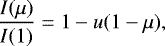 (1)
(1)
the quadratic law (Kopal 1950)
 (2)
(2)
the square-root law (Díaz-Cordovés & Giménez 1992)
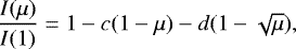 (3)
(3)
the logarithmic law (Klinglesmith & Sobieski 1970)
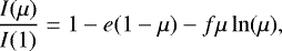 (4)
(4)
the power-2 law (Hestroffer 1997)
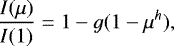 (5)
(5)
and a four-term law (Claret 2000a)
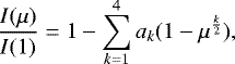 (6)
(6)
where I(1) is the specific intensity at the center of the disk and u, a, b, c, d, e, f, g, h, and ak are the corresponding LDCs. The specific intensities of the model atmosphere were convolved with the transmission curves for the Sloan (u′g′r′i′z′y′), UBV RI, HiPERCAM, Kepler, TESS, and Gaia passbands. It is not straightforward to apply the least-squares method (LSM) to the original 20 μ points because they are not equally spaced. The original distribution can lead to very large weights for the μs near the limb. To avoid this problem, the LDCs were computed for 100 interpolated (equally spaced) μ points instead of 20, as provided originally by the Montréal code described in Tremblay & Bergeron (2009) and Bergeron et al. (2011).
Two numerical methods for computing the LDC are available: LSM and flux conservation (FCM). The advantages and disadvantages of each method are exhaustively discussed in Claret (2000a). Based on this discussion, we here adopted the LSM to adjust the coefficients of Eqs. (1)–(2). For each law, we computed the merit function, given by
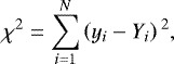 (7)
(7)
where yi is the model intensity at point i, Yi is the fitted function at the same point, and N is the number of μ points. We recall that the biparametric laws are only relatively accurate for some regions of the Hertzsprung-Russel (HR) diagram. Therefore, we recommend adopting Eq. (6) because it meets the following conditions: (a) it uses a single law that is accurate for the whole HR diagram, (b) it is capable of reproducing the intensity distribution very well, (c) the flux is conserved within a very small tolerance, (d) it is applicable to different filters as well as to monochromatic values, and (e) it is applicable to different chemical compositions, effective temperatures, local gravities, and microturbulent velocities.
The biparametric laws (Eqs. (2)–(5)) cannot reproduce the intensity distribution accurately along the HR diagram, although they do it better than the linear law. When these laws are able to represent the intensity distributions well, they are only marginally accurate in certain intervals of effective temperatures and/or log g (see Figs. 4 and 5). As a consequence, the user has to divide the HR diagram into areas of laws in order to use the LDC adequately (see below). Moreover, Eq. (6) provides merit functions of the order of 2 magnitudes smaller than any of the laws quoted previously, mainly in regions close to the limb, as we describe in the next paragraph.
Figures 1 and 2 display the relative differences between the intensities from the model and those from the adjustments given by [I(model) − I(fit)]∕I(model) as a function of μ for two cases: the four-term law (Fig. 1) and the power-2 law (Fig. 2). The two figures are on the same scale to facilitate comparison. The superiority of the four-term law over the power-2 law is clear and the relative differences provided by this approach may be of some orders of magnitude smaller than those corresponding to the power-2 law, mainly near the limb. When we compare the quality of the adjustments using Eq. (6) with those from the other biparametric laws, the quality of the adjustments provided in the first one is still even better than in the case of the power-2 law.
In order to avoid a biased interpretation of the quality of the adjustments illustrated in Figs. 1 and 2, we include in Figs. 3 and 4 the merit function for all DA models and all six Sloan passbands adopted in this study. A direct comparison between these two figures shows that the fit quality of the four-term law is always far higher than that of the power-2 law (almost 2 orders of magnitude). They are only similar in the interval 4.4–4.6 in log Teff, but even so, the four-term law is superior. In this interval the specific intensities behave more smoothly, which explains the similarity in the behavior of the merit function of these two laws.
For the biparametric laws alone, we illustrate in Fig. 5 the behavior of the square-root law for the same conditions as in Figs. 3 and 4. The χ2 provided by the power-2 law is similar to those given by the square-root law. The square-root law provides smaller χ2 than the power-2 law for DB models, showing lower effective temperatures. When a biparametric law is to be adopted, we therefore recommend an inspection of the values of the merit function for each law, for each model, and for each passband to select the most accurate.
It has been known for a long time that the linear law does not adequately describe the distribution of specific intensities when realistic stellar atmosphere models are used. Despite this deficiency, this law can be used, for example, to compare models with different input physics. In Fig. 6 we compare the linear LDC for the DB, DA, and DBA models to analyze the effect of the hydrogen content on the distribution of specific intensities for a constant value of log g = 7.00. Theinfluence of hydrogen content on the slope is clear: DBA models have higher LDCs up to Teff ≈ 20 000 K, while the opposite occurs for higher effective temperatures. For the DA models, LDCs show an almost linear dependence on effective temperature. Only the DA and DBA models have similar LDCs for a narrow range of effective temperatures (10 900–15 500 K, and this is within the semi-empirical errors). On the other hand, it is important to note that the global differences in the LDC for the three sets of models are larger or of the order than the typical semi-empirical errors that can be derived in the case of high-quality light curves. As a consequence, the three types of white dwarfs investigated here might be distinguishable observably using the appropriate LDCs.
As mentioned, the linear approximation is not very adequate, but on the other hand, it facilitates visualizing the differences between the LDCs that were computed from different model grids. A comparison of our results with the previous ones from Gianninas et al. (2013) is a good consistency check. In Fig. 7 we show this comparison for the g filter. The agreement between the two computations is very good, and the small differences may be due to the modifications that have recently been introduced in the code and numerical precision.
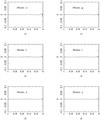 |
Fig. 1 Relative differences Δ ≡ [I (model) − I (fit)]/I (model) as a function of μ for the Sloanpassbands. Four-term law, log g = 5.5, Teff = 10 000 K, and DA models (LTE). |
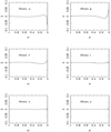 |
Fig. 2 Relative differences Δ ≡ [I (model) − I (fit)]/I (model) as a function of μ for the Sloanpassbands. Power-2 law, log g = 5.5, Teff = 10 000 K, and DA models (LTE). |
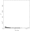 |
Fig. 3 Merit function χ2 for all models of the sample. Four-term law, all Sloan passbands, and DA models (LTE). |
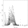 |
Fig. 4 Merit function χ2 for all models of the sample. Power-2 law, all Sloan passbands, and DA models (LTE). |
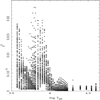 |
Fig. 5 Merit function χ2 for all models of the sample. Square root-law, all Sloan passbands, and DA models (LTE). |
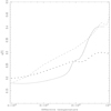 |
Fig. 6 Linear LDC as a function of the effective temperature for the V passband. Asterisks denote DB models, DBAs (LTE) are represented by the continuous line, and the dashed line indicates DA models. Log g = 7.0. |
 |
Fig. 7 Comparison between our linear LDCs (continuous line) and those computed by Gianninas et al. (2013), which are denoted by asterisks. DA models, log g = 6.0. |
4 Calculating the gravity-darkening coefficients
As is well known, rotation and/or tides distort the shapes of stars. Such distortions have been investigated by Kopal (1959), who used spherical harmonics to describe them. The studies are in particular important in close binary systems or in planetary systems where both mechanisms act simultaneously: tides tend to elongate the star, while rotation tends to flatten it at the poles. The corresponding deviations from a sphere are functions of the rotational rates and of the mass ratio q. A mathematical summary will help us understand the results obtained by Kopal. Consider the total potential of a rotating star. We assume that the angle between the normal and the radius vector is small and that only the radial component of the derivative is considered to compute the local gravity. Thus, we have
 (8)
(8)
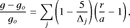
where go is the local gravity (taken as reference), Δj = 1 + 2kj and kj is the apsidal motion constant of order j. For j = 2, the radius of an equipotential r can be written as
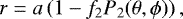 (9)
(9)
where f2 is given by
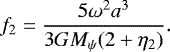 (10)
(10)
In the above equation ω is the angular velocity, P2(θ, ϕ) is the second surface harmonic, a is the mean radius of the level surface, η2 is the logarithmic derivative of the spherical harmonic defined through Radau’s equation, and Mψ is the mass enclosed by an equipotential. The importance of Eq. (10) is that it establishes a dependence of the GDE on the shape of the distorted stellar configuration, on its internal structure, and also on the details of the rotation law. More details on these calculations have been presented by Claret (2000b).
From the physical point of view, more than the geometrical changes must be considered. von Zeipel (1924) showed that for configurations in pure radiative equilibrium (pseudo-barotrope), the emerging flux is not constant on the surface of a distorted star and depends on the value of the local gravity:
 (11)
(11)
or
 (12)
(12)
where g is the local gravity, Φ is the total potential, T is the local temperature, κ is the opacity, ρ is the local density, a is the radiation pressure constant, c the velocity of light in vacuum, Teff is the effective temperature, and β1 = 1.0 is the GDE, a bolometric quantity.
However, significant deviations from von Zeipel’s theorem have been found when the GDEs are calculated at the upper layers of a distorted star (Claret 2012). This is a consequence of using a transfer equation that is more elaborate than the diffusion approach that was adoptedby von Zeipel (1924). This theorem is therefore not strictly valid at lower optical depths. For details on the calculations of β1, recent results and different methods, see for example, Claret (2012, 2016) and Zorec et al. (2017). The non-validity of von Zeipel’s theorem also extends to compact stars. As previously commented in the Introduction, Claret (2015) used a perturbation theory and derived an equation for the GDE for neutron stars as a function of the rotation law, of the colatitude, and of the logarithmic derivatives of the opacity. This equation predicts significant deviations from the von Zeipel’s theorem for differentially rotating neutron stars.
Concerning the passband gravity-darkening coefficients y(λ) (GDC), Kopal (1959) assumed a simple but ingenious approach six decades ago in the absence of reliable atmosphere models: the distorted configurations radiate like a blackbody. By expanding the ratio between the monochromatic and total radiation in a Taylor series, he derived the GDC as a function of the temperature (effective) and of the wavelength. Of course, the blackbody radiation is not a good approximation, and more elaborate atmosphere models are needed to permit a consistent light-curve analysis. Later, Martynov (1973) refined the calculation of the GDC introducing the following equation:
![Mathematical equation: \begin{eqnarray*}y(\lambda, T_{\textrm{eff}}, \log [\textrm{H/He}], \log g) = \frac{1}{4} \left(\frac{\partial\ln I_o(\lambda)} {\partial\ln T_{\textrm{eff}}}\right)_{g}, \end{eqnarray*}](/articles/aa/full_html/2020/02/aa37326-19/aa37326-19-eq14.png) (13)
(13)
where λ is the wavelength, log [H/He] is the content of hydrogen relative to the content of helium, Io (λ) is the specific intensity at a given wavelength at the center of the stellar disk, and the subscript g indicates a derivative at constant surface gravity. At that time and for many years, the blackbody approach was used to calculate the partial derivative. We also note that Eq. (13) also presents some simplifications. The factor 1/4 indicates that in its derivation, β1 was assumed to be 1.0 for any effective temperature. However, as we previously commented, β1 is a function of the physical conditions in the upper layers and can be different from 1.0, mainly for stars presenting convective envelopes (see below).
Claret & Bloemen (2011) considered the effects of the partial derivative  and of more realistic stellar atmosphere models (PHOENIX and ATLAS) in calculating the GDC,
![Mathematical equation: \begin{align*} &y(\lambda, T_{\textrm{eff }}, \log [\textrm{H/He}], \log g,\!) \nonumber \\[4pt] &\quad=\left(\frac{\textrm{d}\ln T_{\textrm{eff }}}{{\textrm{d}\ln g}}\right) \left(\frac{\partial{\ln I_o(\lambda)}}{{\partial{\ln T_{\textrm{eff }}}}}\right)_{g} + \left(\frac{\partial{\ln I_o(\lambda)}} {\partial{\ln g}}\right)_{T_{\textrm{eff}}}. \end{align*}](/articles/aa/full_html/2020/02/aa37326-19/aa37326-19-eq16.png) (14)
(14)
Following the arguments presented above, the term  can be written as β1∕4, and finally we have
![Mathematical equation: \begin{align*}&y(\lambda, T_{\textrm{eff }}, \log [\textrm{H/He}], \log g) \nonumber \\[4pt] &\quad=\left(\frac{\beta_1}{4}\right) \left(\frac{\partial{\ln I_o(\lambda)}}{{\partial{\ln T_{\textrm{eff }}}}}\right)_{g} + \left(\frac{\partial{\ln I_o(\lambda)}} {\partial{\ln g}}\right)_{T_{\textrm{eff}}}. \end{align*}](/articles/aa/full_html/2020/02/aa37326-19/aa37326-19-eq18.png) (15)
(15)
We used thesame DA, DB, and DBA models as described in Sect. 2 to compute the GDC for all passbands considered here. The corresponding GDC tables consist of two lines per model: the first line refers to the first term of Eq. (15) considering β1 = 1.0, and the second line refers to the second term of this equation. We chose to separate the two contributions so that the value of β1 can be adjusted during the synthesis of the light curves. In this case, the first term only needs to be multiplied by the value of β1 to be iterated.
Figures 8 and 9 (DB and DBA, respectively) show the comparison between the GDC given by Eq. (15) (continuous line) and those calculated using the blackbody approach (asterisks). As anticipated, the blackbody radiation is not a good approximation. This is particularly valid for passbands with short effective wavelengths. Similar effects have been detected in main-sequence and giant stars (see Fig. 4 in Claret 2003). The influence of the second term in the GDC in Eq. (15) is not important, but not negligible (see the second lines of the corresponding tables). We also detected a decrease in GDC for all Sloan passbands around 20 000 K for the DB and DBA models. This feature might be connected to the onset of He II convection (Cukanovaite et al 2019).
As explained in Sect. 2, we also computed DA NLTE models. GDC calculations can serve as an indicator (although not the definitive) of the effective temperature limit for which it is necessary to adopt NLTE. Figure 10 shows the comparison between LTE (continuous line) and NLTE (asterisks) models. For all Sloan filters, this effective temperature limit is at about 40 000 K, in good agreement with previous estimates (Gianninas et al. 2013). This effective temperature is practically independent of local gravity. The systematic and small offsets that we show in Fig. 10 at lower effective temperatures are probably due to the use of different codes for LTE and NLTE. Therefore, we can conclude that the effect of considering NLTE is practically negligible in GDC calculations. A discussion for the onset of NLTE effects can be found in Liebert et al. (2005).
Because 1D convection is limited, the theoretical GDC (DA models) for Teff = 5000 K show some discontinuities at the shortest wavelengths (passbands u and U). We have preferred to keep these discontinuities in the respective tables and leave the task of smoothing them to the user according to
their needs.
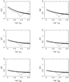 |
Fig. 8 Theoretical gravity-darkening coefficients for the SLOAN passbands (DB models). The continuous line represents the calculations for log g = 8.0, and asterisks denote the calculations by adopting the blackbody approach. |
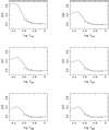 |
Fig. 10 Effects of NLTE on the GDC (DA models). The continuous line indicates LTE models, and asterisks denote NLTE models. Sloan passbands. Log g = 8.25. |
Acknowledgements
We thank the anonymous referee for helpful comments that have improved the manuscript. The Spanish MEC (AYA2015-71718-R and ESP2017-87676-C5-2-R) is gratefully acknowledged for its support during the development of this work. A.C. also acknowledges financial support from the State Agency for Research of the Spanish MCIU through the “Center of Excellence Severo Ochoa” award for the Instituto de Astrofísica de Andalucía (SEV-2017-0709). The research leading to these results has received funding from the European Research Council under the European Union’s Horizon 2020 research and innovation programme n. 677706 (WD3D). This research has made use of the SIMBAD database, operated at the CDS, Strasbourg, France, and of NASA’s Astrophysics Data System Abstract Service.
Appendix A Brief description of Tables A.1–A.3
In order to provide users with the complementary tools for the synthesis of light curves, we also computed the Doppler beaming for each photometric system. The Doppler beaming factors adopting the BB approach were computed according to Eq. (3) (parameter α) in Loeb & Gaudi (2003). Tables A.1–A.3 summarize the type of data available as well as the central intensities for each photometric system in ergs cm−2 s−1 Hz−1 ster−1, and the Doppler beaming for the BB approach. For more details, see the ReadMe file at the CDS.
Gravity and limb-darkening coefficients for the Sloan and UBVRI photometric systems.
Gravity and limb-darkening coefficients for the HiPERCAM photometric system.
Gravity and limb-darkening coefficients for the Kepler, TESS, and Gaia photometric systems.
References
- Bergeron, P., Wesemael, F., Dufour, P., et al. 2011, ApJ, 737, 28 [NASA ADS] [CrossRef] [EDP Sciences] [Google Scholar]
- Brown, W. R., Kilic, M., Allende Prieto, C., et al. 2010, ApJ, 723, 1072 [NASA ADS] [CrossRef] [Google Scholar]
- Burdge, K. B., Coughlin, M. W., Fuller, J., et al. 2019a, Nature, 571, 528 [NASA ADS] [CrossRef] [Google Scholar]
- Burdge, K., Fuller, J., Phinney, E. S., et al. 2019b, ApJ, 886, L12 [NASA ADS] [CrossRef] [Google Scholar]
- Claret, A. 2000a, A&A, 363, 1081 [NASA ADS] [Google Scholar]
- Claret, A. 2000b, A&A, 359, 289 [NASA ADS] [Google Scholar]
- Claret, A. 2003, A&A, 406, 623 [NASA ADS] [CrossRef] [EDP Sciences] [Google Scholar]
- Claret, A. 2012, A&A, 538, A3 [NASA ADS] [CrossRef] [EDP Sciences] [Google Scholar]
- Claret, A. 2015, A&A, 577, A87 [NASA ADS] [CrossRef] [EDP Sciences] [Google Scholar]
- Claret, A. 2016, A&A, 588, A15 [NASA ADS] [CrossRef] [EDP Sciences] [Google Scholar]
- Claret, A., & Bloemen, S. 2011, A&A, 529, A75 [NASA ADS] [CrossRef] [EDP Sciences] [Google Scholar]
- Cukanovaite, E., Tremblay, P.-E., Freytag, B., et al. 2019, MNRAS, 490, 1010 [NASA ADS] [CrossRef] [Google Scholar]
- Dhillon, V. S., Marsh, T. R., Stevenson, M. J., et al. 2007, MNRAS, 378, 825 [NASA ADS] [CrossRef] [MathSciNet] [Google Scholar]
- Dhillon, V. S., Dixon, S., Gamble, T., et al. 2018, Proc. SPIE, 10702, 107020L [Google Scholar]
- Díaz-Cordovés, J., & Giménez, A. 1992, A&A, 259, 227 [NASA ADS] [Google Scholar]
- Gianninas, A., Strickland, B. D., Kilic, M., & Bergeron, P. 2013, ApJ, 765, 102H [NASA ADS] [CrossRef] [Google Scholar]
- Hallakoun, N., Xu, S., Maoz, D., et al. 2018, MNRAS, 469, 3213 [NASA ADS] [CrossRef] [Google Scholar]
- Hermes, J. J., Kilic, M., Brown, W. R., et al. 2012, ApJ, 757, L21 [NASA ADS] [CrossRef] [Google Scholar]
- Hestroffer, D. 1997, A&A, 327, 199 [NASA ADS] [Google Scholar]
- Hubeny, I., & Lanz, T. 1995, ApJ, 439, 875 [Google Scholar]
- Klinglesmith, D. A., & Sobieski, S. 1970, AJ, 75, 175 [NASA ADS] [CrossRef] [Google Scholar]
- Kopal, Z. 1950, Harv. College Observ. Circ., 454, 1 [NASA ADS] [Google Scholar]
- Kopal, Z. 1959, Close Binary Systems (London: Chapman & Hall) [Google Scholar]
- Liebert, J., Bergeron, P., & Holberg, J. B. 2005, ApJS, 156, 47 [NASA ADS] [CrossRef] [Google Scholar]
- Littlefair, S. P., Casewell, S. L., Parsons, S. G., et al. 2014, MNRAS, 445, 2106 [NASA ADS] [CrossRef] [Google Scholar]
- Loeb, A., & Gaudi, B. S. 2003, ApJ, 588, L117 [NASA ADS] [CrossRef] [Google Scholar]
- Martynov, D. Ya. 1973, in Eclipsing Variable Stars, ed. V. P. Tsesevich, IPST Astrophys. Lib. (New Jersey: John Wiley & Sons), 128 [Google Scholar]
- McAllister, M., Littlefair, S. P., Parsons, S. G., et al. 2019, MNRAS, 486, 5535 [NASA ADS] [CrossRef] [Google Scholar]
- Milne, E.A. 1921, MNRAS, 81, 361 [NASA ADS] [CrossRef] [Google Scholar]
- Parsons, S. G., Gänsicke, B. T., Marsh, T. R., et al. 2017, MNRAS, 470, 4473 [NASA ADS] [CrossRef] [Google Scholar]
- Rebassa-Mansergas, A., Parsons, S. G., Dhillon, V. S., et al. 2019. Nat. Astron., 3, 553 [NASA ADS] [CrossRef] [EDP Sciences] [Google Scholar]
- Russell, H. N. 1912, ApJ, 36, 54 [NASA ADS] [CrossRef] [Google Scholar]
- Schwarzschild, K. 1906, Nachrichten von der Gesellschaft der Wissenschaften zu Gottingen, Mathematisch-Physikalische Klasse (Charleston: Nabu Press), 43 [Google Scholar]
- Tremblay, P.-E., & Bergeron, P. 2009, ApJ, 696, 1755 [NASA ADS] [CrossRef] [Google Scholar]
- Tremblay, P.-E., Bergeron, P., Kalirai, J. S., & Gianninas, A. 2010, ApJ, 712, 1345 [NASA ADS] [CrossRef] [Google Scholar]
- Tremblay, P.-E., Ludwig, H.-G., Steffen, M., et al. 2013, A&A, 559, A104 [NASA ADS] [CrossRef] [EDP Sciences] [Google Scholar]
- von Zeipel, H. 1924, MNRAS, 84, 665 [NASA ADS] [CrossRef] [Google Scholar]
- Zorec, J., Rieutord, M., Espinosa Lara, F., et al. 2017, A&A, 606, A32 [NASA ADS] [CrossRef] [EDP Sciences] [Google Scholar]
All Tables
Gravity and limb-darkening coefficients for the Sloan and UBVRI photometric systems.
Gravity and limb-darkening coefficients for the Kepler, TESS, and Gaia photometric systems.
All Figures
|
Fig. 1 Relative differences Δ ≡ [I (model) − I (fit)]/I (model) as a function of μ for the Sloanpassbands. Four-term law, log g = 5.5, Teff = 10 000 K, and DA models (LTE). |
| In the text | |
|
Fig. 2 Relative differences Δ ≡ [I (model) − I (fit)]/I (model) as a function of μ for the Sloanpassbands. Power-2 law, log g = 5.5, Teff = 10 000 K, and DA models (LTE). |
| In the text | |
|
Fig. 3 Merit function χ2 for all models of the sample. Four-term law, all Sloan passbands, and DA models (LTE). |
| In the text | |
|
Fig. 4 Merit function χ2 for all models of the sample. Power-2 law, all Sloan passbands, and DA models (LTE). |
| In the text | |
|
Fig. 5 Merit function χ2 for all models of the sample. Square root-law, all Sloan passbands, and DA models (LTE). |
| In the text | |
|
Fig. 6 Linear LDC as a function of the effective temperature for the V passband. Asterisks denote DB models, DBAs (LTE) are represented by the continuous line, and the dashed line indicates DA models. Log g = 7.0. |
| In the text | |
|
Fig. 7 Comparison between our linear LDCs (continuous line) and those computed by Gianninas et al. (2013), which are denoted by asterisks. DA models, log g = 6.0. |
| In the text | |
|
Fig. 8 Theoretical gravity-darkening coefficients for the SLOAN passbands (DB models). The continuous line represents the calculations for log g = 8.0, and asterisks denote the calculations by adopting the blackbody approach. |
| In the text | |
 |
Fig. 9 Effects of hydrogen content on the GDC (DBA models). The captions are the same as for Fig. 8. |
| In the text | |
|
Fig. 10 Effects of NLTE on the GDC (DA models). The continuous line indicates LTE models, and asterisks denote NLTE models. Sloan passbands. Log g = 8.25. |
| In the text | |
Current usage metrics show cumulative count of Article Views (full-text article views including HTML views, PDF and ePub downloads, according to the available data) and Abstracts Views on Vision4Press platform.
Data correspond to usage on the plateform after 2015. The current usage metrics is available 48-96 hours after online publication and is updated daily on week days.
Initial download of the metrics may take a while.