| Issue |
A&A
Volume 631, November 2019
|
|
|---|---|---|
| Article Number | A31 | |
| Number of page(s) | 12 | |
| Section | The Sun | |
| DOI | https://doi.org/10.1051/0004-6361/201936198 | |
| Published online | 15 October 2019 | |
Effect of siphon flow on resonant damping of kink oscillations in magnetic flux tubes
1
School of Mathematics and Statistics (SoMaS), The University of Sheffield, Hicks Building, Hounsfield Road, Sheffield S3 7RH, UK
e-mail: This email address is being protected from spambots. You need JavaScript enabled to view it.
2
Space Research Institute (IKI) Russian Academy of Sciences, Moscow, Russia
3
National Research University Higher School of Economics, Moscow, Russia
Received:
27
June
2019
Accepted:
5
August
2019
Abstract
The effect of siphon flow on kink oscillations of magnetic flux tubes is studied in the thin tube and thin boundary layer (TTTB) approximation. The presence of a transitional layer results in oscillation damping due to resonance absorption. To calculate the damping rate we use the regular perturbation method with the ratio of transitional layer thickness to tube radius as a small parameter. We found a dependence of the ratio of decrement to the oscillation frequency, γ/ω1, on the ratio, χ, of flow velocity magnitude to the Alfvén speed in the tube core. The general theoretical results are applied to a particular case where the density radial dependence in the transitional layer is linear. We consider two models. In the first model, the radial dependence of the velocity amplitude is such that the resonance in the transitional layer occurs where the flow velocity is zero. In the second model, the flow velocity is non-zero in the whole transitional layer. In both cases, γ/ω1 is an increasing function of χ. In the first case, the presence of flow can lead to an increase in γ/ω1 by more than a factor of two. In the second model, we only carry out the calculation in the case where the plasma density inside the tube is much larger than the density of the surrounding plasma. In this model, the effect of flow is less pronounced than in the first model, and the presence of flow can increase γ/ω1 by a factor of 0.25 at most. We discuss the application of the obtained results to coronal and prominence seismology. We conclude that while for typical values of velocity in coronal loops the effect of flow is weak, it can be quite substantial in prominence seismology.
Key words: magnetohydrodynamics (MHD) / plasmas / waves / Sun: corona / Sun: magnetic fields / Sun: oscillations
© ESO 2019
1. Introduction
Kink oscillations of coronal magnetic loops were among the first magnetohydrodynamic oscillations observed by space missions in the solar atmosphere at the end of the last century. They were first observed by the Transition Region and Coronal Explorer (TRACE) mission in 1998 and reported by Aschwanden et al. (1999) and Nakariakov et al. (1999). Since then these oscillations have been routinely observed by space missions (e.g. Erdélyi & Taroyan 2008; Duckenfield et al. 2018; Su et al. 2018; Abedini 2018, and references therein). Recently, kink oscillations have also been observed in prominence threads (e.g. Arregui et al. 2018).
Even the first observation of a coronal loop kink oscillation showed that it was strongly damped, with a damping time of a few oscillation periods. At present, it is generally accepted that this damping is caused by resonant absorption. Resonant absorption was first suggested for complimentary plasma heating in fusion devises (Tataronis & Grossmann 1973; Grossmann & Tataronis 1973). At the same time resonant absorption was used to explain the mechanism of magnetospheric pulsations (Lanzerotti et al. 1973; Southwood 1974; Chen & Hasegawa 1974a,b).
After Ionson (1978) proposed resonant absorption as a mechanism for heating coronal magnetic loops, it remained very popular in solar physics. At first, the main effort of researchers was to elaborate the idea by Ionson (1978) and study the coronal heating by resonant absorption of magnetohydrodynamic (MHD) waves (e.g. Kuperus et al. 1981; Ionson 1985; Hollweg 1990). Resonant absorption was also used to explain the observed loss of acoustic power in sunspots (e.g. Hollweg 1988; Lou 1990; Stenuit et al. 1993).
The launch of space missions at the end of the last century boosted the interest of theoretical physicists in studying waves in the solar atmosphere in general, and in application of resonant absorption to problems in solar physics in particular. Nakariakov et al. (1999) suggested that the observed damping of coronal loop kink oscillations was caused by resonant absorption. Ruderman & Roberts (2002) elaborated this idea and showed that the observed oscillation period and damping time can be used to obtain information about the transversal density distribution in a coronal magnetic loop. Goossens et al. (2002) then applied the method suggested by Ruderman & Roberts (2002) to 11 events of coronal loop kink oscillations. Now, this method is among the main methods of a new branch of solar physics called coronal seismology (e.g. Goossens et al. 2006, 2011).
Observations by Solar and Heliospheric Observatory SoHO (Brekke et al. 1997; Winebarger et al. 2002; Teriaca et al. 2004), TRACE (Winebarger et al. 2001; Doyle et al. 2006), and more recently Hinode (Teriaca et al. 2004; Tian et al. 2008; Ofman & Wang 2008) and STEREO (Tian et al. 2009) showed that flows are ubiquitous in active region loops. Flows with speeds of between about 5 km s−1 and 30 km s−1 are also often observed in prominence threads (Chae et al. 2008; Terradas et al. 2008). In view of these observations it is important to study the effect of flow on resonant damping of kink waves in magnetic flux tubes. To our knowledge, Goossens et al. (1992) were the first to address this problem. These latter authors considered kink oscillations of a twisted magnetic tube in the presence of helical flow and derived so-called connection formulae. Using these formulae they studied resonant damping of propagating kink waves in the thin tube and thin boundary layer (TTTB) approximation. Their analysis was extended by Terradas et al. (2010) who studied the damping of propagating kink waves in the TTTB approximation analytically, and without using this approximation numerically. Soler et al. (2011) used the TTTB approximation to study the effect of flow on spatial damping of propagating kink waves analytically, and then studied the same problem numerically without using the TTTB approximation. They compared the analytical and numerical solutions to outline the limit of applicability of the TTTB approximation. Bahari (2018) studied the effect of magnetic twist on the spatial damping of kink waves in the presence of flow.
Terradas et al. (2010) also addressed the problem of resonant damping of standing waves in the presence of flow. However, these latter authors only obtained an approximate solution under the assumption that the flow speed is much smaller than the Alfvén speed in a magnetic tube. They even cast doubt on the possibility of obtaining an exact solution describing a standing wave in the presence of flow. Nevertheless, Ruderman (2010) obtained the solution describing a standing kink wave in a magnetic flux tube in the presence of flow in the thin tube approximation. This solution is a superposition of two waves propagating in different directions. These waves have the same frequency, but different wave numbers. A similar approach was then used by Terradas et al. (2011) who considered an application to coronal seismology. Both Ruderman (2010) and Terradas et al. (2011) considered straight magnetic tubes. Later, Bahari (2017) extended the theory of standing waves in the presence of flow to twisted magnetic tubes. However, all these authors considered a tube with the sharp boundary and thus did not study the resonant wave damping. Therefore, up to now, there have been no studies of the flow effect on resonant damping of standing kink waves that is valid for arbitrary flow velocity. This paper aims to fill this gap.
The paper is organised as follows. In the following section we formulate the problem. The damping rate due to resonant absorption is calculated using the regular perturbation method with the ratio of thickness of the transitional layer to the tube radius used as a small parameter. In Sect. 3 we calculate the first-order approximation. In Sect. 4 we calculate the second-order approximation and thus find the expression for the decrement. In Sect. 5 we apply the general theory to a particular equilibrium with the linear density profile in the transitional region. In Sect. 6 we discuss a possible application of the obtained results to the coronal and prominence seismology. Section 7 contains the summary of obtained results and our conclusions.
2. Problem formulation and governing equations
We consider the plasma motion in the cold plasma approximation. The unperturbed magnetic field is straight in cylindrical coordinates r, ϕ, z, and is given by B = Bez, where ez is the unit vector in the z-direction and B is a constant. In the unperturbed state there is also the plasma flow with the velocity U = U(r)ez. The equilibrium density is given by
 (1)
(1)
where R is the tube radius, ρi and ρe are constants, ρe < ρi, ρt(r) is a monotonically decreasing function, and ρ(r) is continuous at r = R(1 ± l/2). The domain defined by r ≤ R(1 − l/2) is the core part of the magnetic tube, while R(1 − l/2)≤r ≤ R(1 + l/2) defines the transitional region. The velocity magnitude is given by
 (2)
(2)
where Ut(r) is a monotonically decreasing function, and U(r) is continuous at r = R(1 ± l/2). We can always choose the direction of the z-axis in such a way that Ui > 0. Since the magnetohydrodynamic equations are invariant with respect to the substitution B → −B we can assume that B > 0. The equilibrium configuration is shown in Fig. 1.
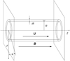 |
Fig. 1. Equilibrium configuration. The magnetic field is the same everywhere, while the velocity is zero outside the tube. The tube length is L. |
The tube length is L. We assume that the tube is thin, R ≪ L. In addition, we assume that the transitional layer is also thin, l ≪ 1. Hence, we use the TTTB approximation. Ruderman et al. (2017) derived the equation describing kink oscillations of a thin expanding non-stationary magnetic tube in the presence of flow. For a particular equilibrium considered in this paper this equation reduces to
 (3)
(3)
 (4)
(4)
Here ζ = ρi/ρe, η, which is the radial displacement of the tube core, is independent of r,  , and
, and
 (5)
(5)
where ξr is the radial component of the plasma displacement and P the magnetic pressure perturbation. The solution to Eq. (3) must satisfy the boundary conditions
 (6)
(6)
Below, we look for the solution in the form of normal modes and take all dependent variables proportional to exp(−iωt). We then use the regular perturbation method and look for the solution in the form
 (7)
(7)
The variation of P and η across the transitional layer is of the order of l. In accordance with this we introduce the scaled quantities
 (8)
(8)
We then transform Eqs. (3) and (4) to
 (9)
(9)
 (10)
(10)
where we use the ordinary derivative instead of the partial because all quantities now only depend on z.
3. First-order approximation
Collecting terms of the order of unity in Eq. (9) we obtain
 (11)
(11)
where
 (12)
(12)
The solution to Eq. (11) must satisfy the boundary conditions
 (13)
(13)
The general solution to Eq. (11) is
 (14)
(14)
where
 (15)
(15)
Substituting Eq. (14) in the boundary conditions Eq. (13) yields
 (16)
(16)
It follows from these equations that
 (17)
(17)
Since we are solving a linear problem we can choose η1+ arbitrarily. To have the correct dimension we take η1+ = −iη0/2, where η0 is a constant with the dimension of length. The second equation in Eq. (17) implies that qL = πn, where n = 1, 2, …. Subsequently with the aid of Eq. (15) we obtain
 (18)
(18)
Here, n = 1 corresponds to the fundamental mode, and n > 1 to the (n − 1)th overtone. Since we use the thin tube approximation we must restrict our analysis to moderate values of n satisfying the condition n ≤ n0, where n0R ≪ L. When  the tube is subject to the Kelvin–Helmholtz (KH) instability with respect to kink oscillations. Below we assume that
  which, in particular, guarantees that kink oscillations are KH-stable. It is then straightforward to show that ω1 is a monotonically decreasing function of Ui.
Using Eq. (17) we obtain
 (19)
(19)
4. Second-order approximation
Collecting terms of the order of l in Eq. (9) yields
 (20)
(20)
We aim to calculate ω2. For this we need to obtain the expression for  .
.
4.1. Calculation of 
To obtain the expression for  we need to calculate
  and
and  . For this we use the linearised MHD equations. The plasma is assumed to be weakly dissipative. We see below that there is at least one resonant surface in the transitional layer where the frequency of kink oscillation coincides with the Doppler-shifted local Alfvénic frequency. Near this surface there are large gradients of perturbations. This implies that, although we can neglect dissipation almost everywhere, we have to take it into account near the resonant surface. We need dissipation to remove the singularity at the resonant surface. Below we only need the jumps of the radial plasma displacement and the magnetic pressure perturbation across the dissipative layer. The exact form of dissipation and the value of dissipation coefficients only affect the behaviour of solution in the dissipative layer. However, they do not affect the jumps of the radial plasma displacement and the magnetic pressure perturbation (e.g. Ruderman et al. 1995; Goossens et al. 2011). In particular, these jumps would remain the same even if we account for viscosity and neglect resistivity, or account for resistivity and neglect viscosity, or keep both of them. This observation enables us to keep viscosity and neglect resistivity.
Large gradients of perturbations only exist in the radial direction. As a result, we can write the term describing viscosity in the momentum equation in a simplified form as the second derivative with respect to r of the velocity perturbation. Summarising, we write the MHD equations as
 (21)
(21)
 (22)
(22)
Here, ρ = ρt(r), U = Ut(r)ez, v = (vr, vϕ, vz) is the velocity perturbation, b = (br, bϕ, bz) the magnetic field perturbation, P = Bbz/μ0 the magnetic pressure perturbation, ν the kinematic viscosity, and μ0 the magnetic permeability of free space. We do not write the mass conservation equation because it is not used below.
We now introduce the plasma displacement ξ = (ξr, ξϕ, ξz). Its relation with the velocity perturbation can be written in two equivalent forms (e.g. Goossens et al. 1992; Ruderman et al. 2017),
 (23)
(23)
where we take into account that ∇ ⋅ U = 0. Ruderman et al. (2017) used this expression for v in terms of ξ to derive the system of equations for P, ξr, and ξϕ. In the particular case of a non-expanding tube, this system reduces to
 (24)
(24)
 (25)
(25)
 (26)
(26)
The characteristic scales in the r and z directions are R and L, respectively. The characteristic time is L/VAi. Using Eqs. (25) and (26) we then obtain the estimate that  is of the order of ϵ2ξr/R, where ϵ = R/L. This estimate implies that the ratio of the left-hand side of Eq. (24) to its right-hand side is of the order of ϵ2, meaning that the left-hand side of Eq. (24) can be neglected and it can be reduced to
 (27)
(27)
Now, taking the dependent variables proportional to exp(−iωt + iϕ) and eliminating ξϕ we obtain the system of equations for ξr and P,
 (28)
(28)
![Mathematical equation: $$ \begin{aligned} P = r\rho \bigg [V_A^2\frac{\partial ^2}{\partial z^2} - \left(U\frac{\partial }{\partial z} -i\omega \right)^2 + \nu \left(U\frac{\partial }{\partial z} -i\omega \right)\frac{\partial ^2}{\partial r^2}\bigg ]\frac{\partial (r\xi _r)}{\partial r}\cdot \end{aligned} $$](/articles/aa/full_html/2019/11/aa36198-19/aa36198-19-eq38.gif) (29)
(29)
The variation of P in the radial direction in the transitional layer is of the order of lP. We need to calculate the jumps of ξr and P across the transitional layer in the leading-order approximation with respect to l. In accordance with this we can take P = Pi in Eq. (29), where Pi is the value of P at r = R(1 − l/2). We also take ω = ω1. We note that Eqs. (28) and (29) are valid everywhere and not only in the transitional layer. Since in the core region ξr = η(z) and we can take ν = 0 there, it follows from Eq. (29) that in this region
![Mathematical equation: $$ \begin{aligned} P = r\rho _i\bigg [V_{Ai}^2\frac{\mathrm{d}^2\eta }{\mathrm{d}z^2} - \bigg (U_i\frac{\mathrm{d}}{\mathrm{d}z} - i\omega \bigg )^2\eta \bigg ]. \end{aligned} $$](/articles/aa/full_html/2019/11/aa36198-19/aa36198-19-eq39.gif) (30)
(30)
Now, taking into account that R(1 − l/2)≈R in the leading-order approximation with respect to l, we obtain from Eq. (30)
![Mathematical equation: $$ \begin{aligned} P_i = R\rho _i\bigg [V_{Ai}^2\frac{\mathrm{d}^2\eta _1}{\mathrm{d}z^2} - \left(U_i\frac{\mathrm{d}}{\mathrm{d}z} - i\omega _1\right)^2\eta _1\bigg ]. \end{aligned} $$](/articles/aa/full_html/2019/11/aa36198-19/aa36198-19-eq40.gif) (31)
(31)
Substituting this result in Eq. (29) and using the approximation r ≈ R in the transitional layer yields
![Mathematical equation: $$ \begin{aligned}&\bigg [V_A^2\frac{\partial ^2}{\partial z^2} - \left(U\frac{\partial }{\partial z}-i\omega \right)^2 \!\!+ \nu \left(U\frac{\partial }{\partial z}-i\omega _1\right)\!\frac{\partial ^2}{\partial r^2}\bigg ] \frac{\partial (r\xi _r)}{\partial r}= \nonumber \\&\qquad \qquad \qquad \frac{\rho _i}{\rho _t(r)}\bigg [V_{Ai}^2\frac{\mathrm{d}^2\eta _1}{\mathrm{d}z^2} - \left(U_i\frac{\mathrm{d}}{\mathrm{d}z} -i\omega _1\right)^2\eta _1\bigg ]. \end{aligned} $$](/articles/aa/full_html/2019/11/aa36198-19/aa36198-19-eq41.gif) (32)
(32)
We did not substitute ω1 for ω in the second term in brackets on the left-hand side of this equation because, as we see further below, the small correction to ω1 can be important in the dissipative layer. Using Eq. (19) and the variable substitution
 (33)
(33)
we transform Eq. (32) to
 (34)
(34)
where
 (35)
(35)
![Mathematical equation: $$ \begin{aligned} C_1 = \frac{2\pi n}{L}\left[h(V_{Ai}^2 -U_i^2) - U_i\omega _1\right], \end{aligned} $$](/articles/aa/full_html/2019/11/aa36198-19/aa36198-19-eq45.gif) (36)
(36)
 (37)
(37)
When deriving Eq. (34), we neglected terms proportional to the product of ν and derivatives of unperturbed quantities. The solution to Eq. (34) must satisfy the boundary conditions
 (38)
(38)
4.1.1. Solution far from the resonant surface
Usually the observed flows in coronal loops and prominence threads are sub-Alfvénic. In accordance with this, below we assume that Ui < VAi. Since ρt(r) is a monotonically decreasing function, it follows that VA(r) is monotonically increasing. Since, in addition, Ut(r) is monotonically decreasing it follows from our assumption that U(r) < VA(r) in the transitional layer.
Now, we consider the solution sufficiently far from the resonant layer. This enables us to neglect the term proportional to ν in Eq. (34) and reduce it to
 (39)
(39)
Now we consider the differential operator ℳ defined by the differential expression −σ2∂2X/∂z2, and the boundary conditions Eq. (38). It is easy to show that the eigenvalues of this operator are equal to  , where
 (40)
(40)
When r varies from R(1 − l/2) to R(1 + l/2), Ωn(r) monotonically increases from nΩi to nΩe, where
 (41)
(41)
taking into account that, by assumption, U(R(1 + l/2)) = 0. Hence, the operator defined by the left-hand side of Eq. (39) and the boundary conditions, Eq. (38) is invertible if and only if ω ≠ ±Ωn(r) for all r ∈ [R(1 − l/2),R(1 + l/2)] and all n = 1, 2, …. This implies that the Alfvén continuum consists of the infinite union of intervals,
![Mathematical equation: $$ \begin{aligned} \mathfrak{V} = \bigcup _{n=1}^\infty \left(\left[-n\Omega _e,-n\Omega _i\right] \bigcup \left[n\Omega _i,n\Omega _e\right]\right) . \end{aligned} $$](/articles/aa/full_html/2019/11/aa36198-19/aa36198-19-eq52.gif) (42)
(42)
The operator defined by the left-hand side of Eq. (39) and the boundary conditions of Eq. (38) can be written as ω2 − ℳ. When ω1 ∉ 𝔙 the solution to the equation (ω2 − ℳ)X = f(z) is
![Mathematical equation: $$ \begin{aligned} X&= (\omega ^2 - \mathcal{M})^{-1}f \nonumber \\&= -\frac{1}{\sigma ^2}\bigg (\frac{\sin [\kappa (L-z)]}{\kappa \sin (\kappa L)}\int _0^z f(u)\sin (\kappa u)\,\mathrm{d}u \nonumber \\&\quad - \frac{\sin (\kappa z)}{\kappa \sin (\kappa L)}\int _z^L f(u)\sin [(\kappa (L-u)]\,\mathrm{d}u\bigg ) , \end{aligned} $$](/articles/aa/full_html/2019/11/aa36198-19/aa36198-19-eq53.gif) (43)
(43)
where κ = ω/σ. Substituting f(z) equal to the right-hand side of Eq. (39) we obtain
![Mathematical equation: $$ \begin{aligned} X&= \frac{i\eta _0 V_A}{\sigma V_{Ai}^2\sin (\kappa L)}\sum _{j=1}^2 \frac{A_j}{\kappa ^2 - \kappa _j^2}\big \{\sin (\kappa L)[\cos (\kappa z) \nonumber \\&\quad - \cos (\kappa _j z)] - \sin (\kappa z)[\cos (\kappa L) - \cos (\kappa _j L)] \nonumber \\&\quad + i[\sin (\kappa z)\sin (\kappa _j L) - \sin (\kappa L)\sin (\kappa _j z)]\big \} , \end{aligned} $$](/articles/aa/full_html/2019/11/aa36198-19/aa36198-19-eq54.gif) (44)
(44)
where
 (45)
(45)
This result can be obtained directly solving the ordinary differential equation, Eq. (39), with the boundary conditions of Eq. (38) where r is only present as a parameter.
It is straightforward to see that the expression for X is regular when  . Hence, the only singularity in this expression appears when sin(κL) = 0. This condition is equivalent to ω = πnσ(r)/L for some positive integer n. We write the second term in the expansion for ω with respect to l as the sum of the real and imaginary part, ω2 = ω2r − iγ. We see further below that γ > 0. This implies that the condition ω = πnσ(r)/L is never satisfied. However, sin(kL) = 𝒪(l−1) when ω1 = πnσ(r)/L, which implies that there are large gradients in the vicinity of point rA determined by this equation. Hence, in the vicinity of rA we have to take into account the term proportional to ν on the left-hand side of Eq. (34). The surface defined by the equation r = rA is called the Alfvén resonant surface.
Since Ωi = πσi/L and Ωe = πσe/L, where σi and σe are values of function σ(r) at r = R(1 − l/2) and r = R(1 + l/2), respectively, the condition that there is rA satisfying the equation ω1 = πnσ(rA)/L is equivalent to ω1 ∈ 𝔙. It is easy to show that the condition nΩi < ω1 < nΩe is always satisfied when Ui < VAi and ζ > 1. Hence, ω1 ∈ [nΩi, nΩe] and, consequently, there is at least one resonant surface. Since the intervals constituting the Alfvén continuum can overlap, it is possible that there are a few resonant surfaces.
4.1.2. Connection formulae
We see that there are large gradients in the radial direction at the resonant surface in the solution to ideal MHD equations. Hence, we need to solve dissipative MHD equations in a narrow dissipative layer embracing the resonance surface. To obtain the solution in the transitional layer we match the ideal solution far from the resonant surface and the dissipative solution in two overlap regions to the left and right of the resonant surface. In these overlap regions, both ideal and dissipative solutions are valid. The only quantities related to the dissipative solution that we need to connect to solutions to the ideal MHD equations are the jumps of ξr and P across the dissipative layer. The expressions for these jumps are called the connection formulae. The notion of connection formulae was first introduced by Sakurai et al. (1991). Goossens et al. (1992) derived the connection formulae for propagating waves in the presence of flow, and later Goossens et al. (1995) improved the derivation by Sakurai et al. (1991) and expressed the solution in the dissipative layer in terms of F and G functions.
Here it is worth making an important comment. When there is no flow, we can take all dependent variables proportional to sin(πnz/L). As a result, after that we obtain a 1D problem with all variables only depending on r. Probably the most important point is that Eq. (34) becomes an ordinary differential equation. However, when there is flow the situation is more complex. We managed to construct the solution to Eq. (11) in the form of a standing wave as the superposition of two propagating waves with the same frequency and different wave numbers. However this approach does not work for Eq. (34). It is even not clear if it is possible to obtain the solution to Eq. (34) as a sum of a few functions with prescribed dependence on z.
A natural way to obtain the solution to Eq. (34) is to expand X in the Fourier series:
 (46)
(46)
We also use the expansions
 (47)
(47)
 (48)
(48)
where
![Mathematical equation: $$ \begin{aligned} a_m(r) = \left[(-1)^{n+m}e^{igL} - 1\right]\bigg (\frac{\pi (m - n)C_1 - gLC_2}{g^2 L^2 - \pi ^2(n-m)^2}+ \frac{\pi (m + n)C_1 - gLC_2}{g^2 L^2 - \pi ^2(n+m)^2}\bigg ). \end{aligned} $$](/articles/aa/full_html/2019/11/aa36198-19/aa36198-19-eq60.gif) (49)
(49)
Substituting Eqs. (46) and (47) in Eq. (34) we obtain with the aid of Eq. (48)
 (50)
(50)
where
 (51)
(51)
If ω1 ≠ πmσ(r)/L in the whole transitional layer then the first term on the left-hand side of this equation strongly dominates the terms proportional to ν, which can be neglected. As a result, Xm(r) is given by
 (52)
(52)
where we substituted ω1 for ω because we calculate all quantities in the transitional layer in the leading order approximation with respect to l.
Now we solve Eq. (50) for values of m corresponding to the existence of resonant surfaces. As we have already shown, the resonant layer always exists when m = n. We also point out that there is a possibility of existence of more than one resonant surface. Since VA(r) monotonically increases and U(r) monotonically decreases in the transitional layer, it follows that σ(r) monotonically increases. It then becomes apparent that if there is a resonant surface for m = n2 > n, then there is a resonant surface for any m ∈ [n, n2]. Similarly, if there is a resonant surface for m = n1 < n (in the case where n > 1), then there is a resonant surface for any m ∈ [n1, n]. Where there are resonant surfaces for m ∈ [n1, n2], the mth resonant surface is defined by r = rm, where rm is determined by the equation
 (53)
(53)
Since σ(r) is a monotonically increasing function, it follows that rn2 < rn2 − 1 < … < rn1.
Let m ∈ [n1, n2]. First of all, we notice that the expression for Ym does not contain Xm. In the vicinity of r = rm the function Xk(r) with k ≠ m is given by Eq. (52) and its gradient is much smaller than the gradient of Xm(r). This implies that the third term on the left-hand side of Eq. (50) strongly dominates the second term, and thus the second term can be neglected. Now, following Goossens et al. (1995) we make the variable substitution s = r − rm in Eq. (50). Since the dissipative layer is very thin, we can use the approximate relation
 (54)
(54)
where ω2 = ω2r − iγ. We neglect the term −2ω1ω2r because, in principle, it can be included in the definition of rm causing a small shift in the position of the resonant surface. It practically does not change the solution in the dissipative layer. In contrast, the account of the term proportional to γ can substantially change this solution as was first shown by Ruderman et al. (1995); see also Tirry & Goossens (1996). We can also substitute rm for r in the right-hand side of Eq. (50). Again following Goossens et al. (1995) we introduce the dimensionless variable
 (55)
(55)
Using this variable and Eq. (54) we transform Eq. (50) to
 (56)
(56)
where
 (57)
(57)
The solution to this equation was obtained by Tirry & Goossens (1996); see also Goossens et al. (2011); it reads
 (58)
(58)
where
 (59)
(59)
We now use Eq. (33). In the dissipative layer we can neglect the derivatives of unperturbed quantities. In addition, we substitute R for r in the transitional layer. As a result, using Eq. (46) we transform Eq. (33) to
 (60)
(60)
where U and VA are calculated at r = rm. When m ∉ [n1, n2] the integral of Xm across the dissipative layer is of the order of the thickness of this layer, which is much smaller than lR. Hence, we can neglect this variation and only leave terms in the sum in Eq. (60) with m ∈ [n1, n2]. Moreover, the dissipative layers are separated meaning that we need to leave only one term in this sum when calculating the jump of ξr across a particular dissipative layer. Hence, to calculate the jump of ξr across the dissipative layer embracing the resonant surface r = rm, we can use the reduced Eq. (60),
 (61)
(61)
Using Eqs. (58) and (59) we then obtain
 (62)
(62)
where fm(z) is an arbitrary function, and
 (63)
(63)
The functions FΛ(τ) and GΛ(τ) were introduced by Goossens et al. (2011). When Λ = 0 they coincide with F(τ) and G(τ), respectively. We note that the expression for GΛ(τ) is slightly different from that given by Goossens et al. (2011). However, the two expressions are different by a constant. Since ξr is defined with the accuracy up to an additive function of z, this difference does not affect the expression for ξr.
We define the jump of a function of τ across the dissipative layer as
![Mathematical equation: $$ \begin{aligned} {[}f(\tau ){]} = \lim _{\tau \rightarrow \infty }\{f(\tau ) - f(-\tau )\}. \end{aligned} $$](/articles/aa/full_html/2019/11/aa36198-19/aa36198-19-eq75.gif) (64)
(64)
To calculate [GΛ(τ)] we use the variable substitution u′ = uτ and then drop the prime. As a result we obtain
![Mathematical equation: $$ \begin{aligned} {[}G_\Lambda (\tau ){]}&= -2i\lim _{\tau \rightarrow \infty } \int _0^\infty \frac{\sin (u\tau )}{u} e^{-u^3/3 + \Lambda u} \mathrm{d}u \nonumber \\&= -2i\lim _{\tau \rightarrow \infty }\int _0^\infty \frac{\sin u}{u} e^{-u^3/3\tau ^3 + \Lambda u/\tau } \mathrm{d}u = -i\pi . \end{aligned} $$](/articles/aa/full_html/2019/11/aa36198-19/aa36198-19-eq76.gif) (65)
(65)
Using this result we obtain from Eq. (62)
![Mathematical equation: $$ \begin{aligned}[\xi _r]_m = \frac{\pi \eta _0 a_m(U^2 - V_A^2)}{R\Delta V_{Ai}^2} \exp \left(\frac{i\omega _1 Uz}{U^2 - V_A^2}\right)\sin \frac{\pi mz}{L} , \end{aligned} $$](/articles/aa/full_html/2019/11/aa36198-19/aa36198-19-eq77.gif) (66)
(66)
where all unperturbed quantities are calculated at r = rm. This expression is called the connection formula, first introduced by Sakurai et al. (1991), as stated above. The subscript m indicates that this expression gives the jump of ξr across the dissipative layer embracing the resonant surface r = rm. We note that, when Λ > 1, which is the case for typical coronal conditions, the thickness of the dissipative layer is of the order of l2R, and inside the dissipative layer the behaviour of ξr is strongly oscillatory (Goossens et al. 2011).
We now calculate [P]. It is easy to show that the ratio of the last term to the first term on the right-hand side of in Eq. (28) is of the order of δA/lR, but δA does not exceed the thickness of the dissipative layer, that is δA ≲ l2R. It then follows that the last term is much smaller than the first and can be neglected. Subsequently, we obtain that the jump of P across the dissipative layer is of the order of  times the thickness of the dissipative layer, that is, it is of the order of
  . On the other hand, the variation of P across the transitional layer is of the order of
  , which is by far larger than the jump of P across the dissipative layer. Hence, we can neglect the jump of P across the dissipative layer and write
![Mathematical equation: $$ \begin{aligned}[P]_m = 0 . \end{aligned} $$](/articles/aa/full_html/2019/11/aa36198-19/aa36198-19-eq81.gif) (67)
(67)
A similar result has been obtained in many studies (e.g. Sakurai et al. 1991; Goossens et al. 1995, 2011).
4.1.3. Calculating  and
and 
In the method of matched asymptotic expansions, the solution in the dissipative layer is called the internal solution, and the solution outside of the dissipative layer the external solution. Equation (64) defines the jump of a quantity across the dissipative layer from the point of view of the internal solution. We can also define the jump of a quantity across the dissipation layer from the point of view of the external solution:
![Mathematical equation: $$ \begin{aligned} {[}f(r){]}_m = \lim _{\varepsilon \rightarrow +0}\{f(r_m + \varepsilon ) - f(r_m - \varepsilon )\}. \end{aligned} $$](/articles/aa/full_html/2019/11/aa36198-19/aa36198-19-eq84.gif) (68)
(68)
The two expressions for the jump must coincide.
The transitional layer with the resonant surfaces removed is the union of n2 − n1 + 1 intervals, [R(1 − l/2),rn1), (rn1, rn1 + 1),…(rn2, R(1 + l/2)]. The solution to the ideal MHD equations in the transitional layer is given by
![Mathematical equation: $$ \begin{aligned} \xi _r&= \frac{1}{R}\int _{R(1-l/2)}^r X \exp \left(\frac{i\omega _1 Uz}{U^2 - V_A^2}\right)\mathrm{d}r\prime \nonumber \\&+ \xi _r\big |_{r=R(1-l/2)} , \qquad r \in [R(1-l/2),r_{n_2}], \end{aligned} $$](/articles/aa/full_html/2019/11/aa36198-19/aa36198-19-eq85.gif) (69)
(69)
 (70)
(70)
![Mathematical equation: $$ \begin{aligned} \xi _r&= \frac{1}{R}\int _{R(1+l/2)}^r X \exp \left(\frac{i\omega _1 Uz}{U^2 - V_A^2}\right)\mathrm{d}r\prime \nonumber \\&\quad + \xi _r\big |_{r=R(1+l/2)} , \qquad r \in (r_{n_1},R(1+l/2)], \end{aligned} $$](/articles/aa/full_html/2019/11/aa36198-19/aa36198-19-eq87.gif) (71)
(71)
where m = n1 + 1, n1 + 2, …, n2, X(r, z) is given by Eq. (46) with Xm(r) defined by Eq. (52),  is an arbitrary function, and
  , but otherwise it is arbitrary. Since we calculate ξr in the transitional layer in the leading-order approximation with respect to l, we substituted R for r and ω1 for ω. The function X(r, z) is given by Eq. (44) with ω1 substituted for ω. When n1 = n2 = n, that is there is only one resonant surface, the ideal solution in the transitional layer is given by Eqs. (69) and (71), while Eq. (70) is redundant.
Using Eqs. (68)–(71) we obtain
![Mathematical equation: $$ \begin{aligned} {[}\xi _r{]}_{n_2}&= \bar{\xi }_{rn_2}(z) - \xi _r\big |_{r=R(1-l/2)} \nonumber \\&\quad - \frac{1}{R}\mathcal{P}\int _{R(1-l/2)}^{\bar{r}_{n_2}} X \exp \left(\frac{i\omega _1 Uz}{U^2 - V_A^2}\right)\mathrm{d}r\prime , \end{aligned} $$](/articles/aa/full_html/2019/11/aa36198-19/aa36198-19-eq90.gif) (72)
(72)
![Mathematical equation: $$ \begin{aligned} {[}\xi _r{]}_m&= \bar{\xi }_{rm-1}(z) - \bar{\xi }_{rm}(z) \nonumber \\&\qquad - \frac{1}{R}\mathcal{P}\int _{\bar{r}_m}^{\bar{r}_{m-1}} X \exp \left(\frac{i\omega _1 Uz}{U^2 - V_A^2}\right)\mathrm{d}r\prime , \end{aligned} $$](/articles/aa/full_html/2019/11/aa36198-19/aa36198-19-eq91.gif) (73)
(73)
![Mathematical equation: $$ \begin{aligned} {[}\xi _r{]}_{n_1}&= \xi _r\big |_{r=R(1+l/2)} - \bar{\xi }_{rn_1}(z) \nonumber \\&\quad - \frac{1}{R}\mathcal{P}\int _{\bar{r}_{n_1-1}}^{R(1+l/2)} X \exp \left(\frac{i\omega _1 Uz}{U^2 - V_A^2}\right)\mathrm{d}r\prime , \end{aligned} $$](/articles/aa/full_html/2019/11/aa36198-19/aa36198-19-eq92.gif) (74)
(74)
where again m = n1 + 1, n1 + 2, …, n2, and X(r, z) is given by Eq. (46) with Xm(r) defined by Eq. (52). When n2 = n1 + 1, that is there are only two resonant surfaces, the jumps of the ideal solution through these surfaces are given by Eqs. (72) and (74), while Eq. (73) is redundant. Finally, when n1 = n2 = n, that is there is only one resonant surface, the jump of the ideal solution through this surface is given by
![Mathematical equation: $$ \begin{aligned} {[}\xi _r{]}_n&= \xi _r\big |_{r=R(1+l/2)} - \xi _r\big |_{r=R(1-l/2)} \nonumber \\&\qquad - \frac{1}{R}\mathcal{P}\int _{R(1-l/2)}^{R(1+l/2)} X \exp \left(\frac{i\omega _1 Uz}{U^2 - V_A^2}\right)\mathrm{d}r\prime . \end{aligned} $$](/articles/aa/full_html/2019/11/aa36198-19/aa36198-19-eq93.gif) (75)
(75)
In Eqs. (72)–(75), 𝒫 indicates the Cauchy principal part of an integral. We use this symbol because X has a singularity at r = rm.
Equations (72)–(74) represent n2 − n1 + 1 equations because in Eq. (73), m runs from n1 + 1 to n2 − 1. Taking the sum of all these equations and recalling that the internal and external expressions for the jump of ξr through the dissipative layer must coincide, we obtain, with the aid of Eq. (5),
![Mathematical equation: $$ \begin{aligned} l\widetilde{\delta \eta } = \frac{1}{R}\mathcal{P}\int _{R(1-l/2)}^{R(1+l/2)} X \exp \left(\frac{i\omega _1 Uz}{U^2 - V_A^2}\right)\mathrm{d}r + \sum _{m=n_1}^{n_2}[\xi _r]_m, \end{aligned} $$](/articles/aa/full_html/2019/11/aa36198-19/aa36198-19-eq94.gif) (76)
(76)
where [ξr]m is defined by Eq. (66).
When calculating [P]m we showed that the last term on the right-hand side of Eq. (28) can be neglected in the dissipative layer. Since it can also be neglected outside of the dissipative layer, we conclude that this term can be neglected everywhere in the transitional layer. Since the variation of ξr in the transitional layer is of the order of lη, and ξr = η in the core region, we can substitute η1 for ξr in Eq. (28) in the leading-order approximation with respect to l. We then obtain
 (77)
(77)
Using Eqs. (19) and (67) we obtain from this equation in the leading-order approximation with respect to l:
 (78)
(78)
Now, using Eqs. (19), (66), (76), and (78) we obtain
 (79)
(79)
where
![Mathematical equation: $$ \begin{aligned} \widetilde{\mathcal{L}}_1&= \left(V_{Ai}^2\frac{\mathrm{d}^2}{\mathrm{d}z^2} + \frac{\omega _1^2}{\zeta }\right) \sum _{m=n_1}^{n_2}[\xi _r]_m \nonumber \\&= \frac{\pi \eta _0}{lR} \sum _{m=n_1}^{n_2} \frac{a_m(V_{Am}^2 - U_m^2)}{\Delta _m V_{Ai}^2} \exp \left(\frac{i\omega _1 U_m z}{U_m^2 - V_{Am}^2}\right) \nonumber \\&\quad \times \bigg (M_m\sin \frac{\pi mz}{L} + iN_m\cos \frac{\pi mz}{L}\bigg ), \end{aligned} $$](/articles/aa/full_html/2019/11/aa36198-19/aa36198-19-eq98.gif) (80)
(80)
![Mathematical equation: $$ \begin{aligned} \widetilde{\mathcal{L}}_2&= -\eta _0 e^{-ihz}\bigg [\bigg (S_n\sin \frac{\pi nz}{L} + \frac{2\pi inhV_{Ai}^2}{L}\cos \frac{\pi nz}{L}\bigg )\nonumber \\&\quad + \frac{1}{lR}\bigg (iC_1\cos \frac{\pi nz}{L} + C_2\sin \frac{\pi nz}{L}\bigg )\int _{R(1-l/2)}^{R(1+l/2)}\frac{\rho }{\rho _i}\,\mathrm{d}r\bigg ] , \end{aligned} $$](/articles/aa/full_html/2019/11/aa36198-19/aa36198-19-eq99.gif) (81)
(81)
 (82)
(82)
where
 (83)
(83)
 (84)
(84)
 (85)
(85)
 (86)
(86)
 (87)
(87)
and the subscript m at the unperturbed quantities indicates that they are calculated at r = rm. To derive Eqs. (83) and (84) we used the relation σ(rm) = ω1L/πm.
4.2. Calculation of decrement
The boundary value problem that consists of the homogeneous counterpart of Eq. (20) and the zero boundary conditions has a non-trivial solution η2 = η1. This implies that the inhomogeneous problem has solutions only if its right-hand side satisfies the compatibility condition. In accordance with this condition the right-hand side of Eq. (20) is orthogonal to a solution to the boundary value problem adjoined to that of the first-order approximation. This solution is  , where the asterisk indicates a complex conjugate. To obtain the compatibility condition we multiply Eq. (20) by η1*, integrate the obtained equation with respect to z from 0 to L, and use the integration by parts and the zero boundary conditions. As a result we obtain that the integral of the left-hand side is zero, which implies that the integral of the right-hand side must also be zero. This condition determines ω2:
 (88)
(88)
Using the expression for η1, ω1, and h we transform this equation to
 (89)
(89)
The integral in this expression is evaluated in Appendix A. In particular, it is shown that  is purely imaginary, while
  and
and  are real. Hence, the imaginary part of ω2 is defined by the first integral, and the real part by the second integral. The real part of ω2 only provides a correction of the order of l to the oscillation frequency. We are mainly interested in the decrement γ given by
 (90)
(90)
where ℑ indicates the imaginary part of a quantity. Using Eq. (A.3) we obtain
![Mathematical equation: $$ \begin{aligned} \gamma&= \frac{-L\sqrt{\zeta }}{nRV_{Ai}^2\sqrt{2(\zeta +1)V_{Ai}^2 - U_i^2}} \sum _{m=n_1}^{n_2} \frac{V_{Am}^2 - U_m^2}{\Delta _m} \nonumber \\&\quad \times [1 - (-1)^{n+m}\cos (g_m L)]\left[\frac{g_m LM_m + \pi (n-m)N_m}{g_m^2 L^2 - \pi ^2(n-m)^2} \right. \nonumber \\&\quad - \left. \frac{g_m LM_m - \pi (n+m)N_m}{g_m^2 L^2 - \pi ^2(n+m)^2} \right] \left[\frac{g_m LC_2 - \pi (n-m)C_1}{g_m^2 L^2 - \pi ^2(n-m)^2} \right. \nonumber \\&\quad + \left. \frac{g_m LC_2 - \pi (n+m)C_1}{g_m^2 L^2 - \pi ^2(n+m)^2} \right] . \end{aligned} $$](/articles/aa/full_html/2019/11/aa36198-19/aa36198-19-eq113.gif) (91)
(91)
5. Example: Linear density profile in the transitional layer
In this section, we apply the general theory to a particular case where the density in the transitional layer is a linear function of r. It is defined by
![Mathematical equation: $$ \begin{aligned} \rho _t = \rho _i\left[\frac{\zeta + 1}{2\zeta } + \frac{(\zeta - 1)(R - r)}{lR\zeta }\right]. \end{aligned} $$](/articles/aa/full_html/2019/11/aa36198-19/aa36198-19-eq114.gif) (92)
(92)
We specify the radial dependence of the flow velocity in the transitional layer later. Below we only consider the fundamental mode and take n = 1.
5.1. No flow at resonant surface
We assume that U(r) monotonically decreases from Ui to 0 in the interval [R(1 − l/2),rα] and U(r) = 0 in the interval [rα, R(1 + l/2)]. The resonant surface is defined by r = rA. We assume that rA > rα, that is the resonance surface is in the part of the transitional region where there is no flow, U(rA) = 0. The resonant position is defined by VA(rA) = ω1L/π. It follows from this equation that
![Mathematical equation: $$ \begin{aligned} r_A = R[1 - lf(\chi ,\zeta )], \; f(\chi ,\zeta ) = \chi ^2\frac{4\zeta + 2 - \chi ^2(\zeta + 1)}{2(\zeta - 1)(2 - \chi ^2)^2} , \end{aligned} $$](/articles/aa/full_html/2019/11/aa36198-19/aa36198-19-eq115.gif) (93)
(93)
where χ = Ui/VAi. It is easy to prove that ω1 < 2Ωi, which implies that there is only one resonant surface. The condition that the resonant surface is inside the transitional layer reduces to  . This inequality is equivalent to χ < χmax, where χmax is defined by
 (94)
(94)
When ζ varies from 1 to ∞, χmax monotonically increases from 0 to  , while χmax(3)≈0.64.
When χ > χmax it follows that rA < rα, that is the resonance surface must be in the part of the transitional layer where the flow velocity is non-zero. If U = 0 in the whole transitional layer, that is the internal boundary is a tangential discontinuity, then there is no resonance. When there is no flow while the density continuously decreases in a transitional layer then there is always a resonance surface there. However sufficiently strong flow confined in the core region can shift the kink oscillation frequency out of the Alfvén continuum and eliminate resonance.
In Eq. (91), n = m = 1. Using Eqs. (15), (35)–(37), (54), (83), (84), and (92), we obtain
 (95)
(95)
 (96)
(96)
![Mathematical equation: $$ \begin{aligned} C_2 = \frac{\pi ^2 V_{Ai}^2[\chi ^4 - (\zeta + 3)\chi ^2 - 2(\zeta - 1)]}{L^2(2\zeta + 2 - \chi ^2)}\cdot \end{aligned} $$](/articles/aa/full_html/2019/11/aa36198-19/aa36198-19-eq121.gif) (97)
(97)
Substituting these expressions in Eq. (91) and using Eq. (18) yields
![Mathematical equation: $$ \begin{aligned} \frac{\gamma }{l\omega _1}&= \frac{8[2(\zeta + 1) - \chi ^2][2(\zeta - 1) + 3\chi ^2 - \chi ^4]}{\pi \chi ^2\zeta (\zeta - 1)[8(\zeta + 1) - (\zeta + 4)\chi ^2]^2} \nonumber \\&\quad \times \frac{1 - \cos (g_1 L)}{(2 - \chi ^2)^3}\big [8(\zeta ^2 - 1) - 2(\zeta ^2 - 5\zeta - 8)\chi ^2 \nonumber \\&\quad - (\zeta + 2)(\zeta + 5)\chi ^4 + (\zeta + 2)\chi ^6\big ]\cdot \end{aligned} $$](/articles/aa/full_html/2019/11/aa36198-19/aa36198-19-eq122.gif) (98)
(98)
When χ → 0 we obtain
 (99)
(99)
This expression coincides with one derived previously (e.g. Goossens et al. 2011). We obtain another limiting expression taking ζ → ∞, which is relevant for prominence threads where ζ ≳ 100:
![Mathematical equation: $$ \begin{aligned} \frac{\gamma }{l\omega _1} = \frac{32(4 + \chi ^2)[1 - \cos (\pi \chi /\sqrt{2})]}{\pi \chi ^2(2 - \chi ^2)^2(8 - \chi ^2)^2}\cdot \end{aligned} $$](/articles/aa/full_html/2019/11/aa36198-19/aa36198-19-eq124.gif) (100)
(100)
The dependence of γ/lω1 on χ is shown in Fig. 2 for a few values of ζ and χ ∈ [0, χmax(ζ)]. This dependence with ζ = 100 practically coincides with that given by Eq. (100).
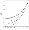 |
Fig. 2. Dependence of γ/lω1 on χ given by Eq. (98). The dash-dotted, long-dashed, short-dashed, and solid curves correspond to ζ = 3, 5, 10, and 100, respectively. The small dark squares show the dependence of γ/lω1 on χ for ζ → ∞ given by Eq. (100). Each curve is shown for χ ∈ [0, χmax]. |
5.2. Equilibrium with flow at the resonant surface
We choose the radial dependence of the velocity in such a way that it will be possible to calculate the resonant position analytically. Hence, we define the flow speed in the transitional layer by
 (101)
(101)
To simplify calculations we assume that ζ ≫ 1, which is relevant in application to prominence threads. Below we calculate all quantities in the leading-order approximation with respect to ζ. We also impose the condition that there is only one resonance surface. This condition is equivalent to ω1 < 2Ωi. In the leading-order approximation with respect to ζ it reduces to ![Mathematical equation: $ \chi < [(6 - 2\sqrt2)/7]^{1/2} \approx 0.673 $](/articles/aa/full_html/2019/11/aa36198-19/aa36198-19-eq126.gif) . It follows from Eq. (18) that
. It follows from Eq. (18) that
 (102)
(102)
We now calculate rA. It is defined by πσ(rA)/ = ω1. Using Eqs. (12), (35), (101), and (102) yields  . Subsequently, using Eq. (92), we obtain rA = R + 𝒪(ζ−1). Using this result and Eqs. (15), (35)–(37), (54), (83), (84), and (92), we obtain in the leading-order approximation with respect to ζ that
 (103)
(103)
 (104)
(104)
 (105)
(105)
Substituting these expressions in Eq. (91) and using Eq. (102) yields
![Mathematical equation: $$ \begin{aligned} \frac{\gamma }{l\omega _1} = \frac{16(1 + \chi ^2)(4 + \chi ^2)[1 - \cos (\pi \chi /\sqrt{2})]}{\pi \chi ^2(2 + \chi ^2)(8 - \chi ^2)^2}\cdot \end{aligned} $$](/articles/aa/full_html/2019/11/aa36198-19/aa36198-19-eq132.gif) (106)
(106)
The dependence of γ/lω1 on χ given by Eq. (106) is shown in Fig. 3. Comparing Figs. 2 and 3 shows that in the first model the effect of flow on the value of γ/lω1 is much more pronounced than in the second. We can give a qualitative explanation to this result. Since we took ζ ≫ 1 in the second model, we also take ζ ≫ 1 in the first model in the following discussion. It follows from Eq. (102) that ω1 is a decreasing function of χ. The increment γ is inversely proportional to Δ. When ω1 decreases, the resonance occurs at lower values of frequencies in the Alfvén continuum. Since the Alfvén frequency monotonically increases with the distance from the inner boundary of the transitional layer, the resonant position is shifted towards the inner boundary in both models. This results in the decrease of Δ and consequently in the increase of γ. However, the presence of flow in the transitional layer in the second model causes the decrease of the Alfvén frequency at each magnetic surface. As a result, the shift of the resonance position towards the inner boundary in the second model is less pronounced than in the first one. As a consequence, the decrease of Δ in the second model is also less pronounced than in the first one, which is confirmed by the fact that Δ is proportional to (2 − χ2)4 in the first model and to 4 − χ4 in the second model. It is straightforward to show that the first function decreases with the increase of χ much faster than the second one. Hence, while the denominator of the expression γ/lω1 is the same in both models, the numerator of this expression in the first model increases with the increase of χ much faster than that in the second model.
6. Application to coronal loops and prominence threads
As already mentioned in Sect. 1, the ratio γ/ω1 is used in coronal seismology to obtain information about the internal structure of magnetic tubes in the solar atmosphere. When there is no siphon flow we can use Eq. (99) to obtain an estimate of the transitional region thickness. Introducing the oscillation period Π = 2π/ω1 and the damping time tdamp = 1/γ, we obtain for the relative thickness of the transitional layer that
 (107)
(107)
Of course, to find l we also need the information on the density contrast ζ.
The typical value of siphon flow velocities observed in coronal magnetic loops is substantially smaller than the Alfvén speed inside these loops, which implies that the correction to l related to the presence of siphon flow is relatively small. However, the situation is different in the case of prominence threads. Due to huge plasma density in threads, the Alfvén speed inside them can be quite low, of the order of 50 km s−1. Hence, we can easily have χ ≃ 0.6. It then follows from the first model studies in Sect. 5.1 that the presence of siphon flow can increase the ratio γ/lω1 up to two times and, consequently, reduce the estimate for l by up to two times. We also note that in a prominence thread ζ ≫ 1, meaning that we do not need to know ζ to estimate l.
In the second model studied in Sect. 5.2, the maximum possible increase in γ/lω1 is only about one quarter and consequently the maximum possible reduction in the estimate of l is also about one quarter. Therefore, in the second model the effect of siphon flow is much less pronounced. At present it is difficult to say which of the two models is more appropriate in the application to prominence threads.
7. Summary and conclusions
In this paper we study the effect of siphon flow on kink oscillations of a magnetic flux tube. We used the thin tube and thin boundary layer (TTTB) approximation, and the approximation of cold plasma. We used the equation describing kink oscillations that was derived by Ruderman et al. (2017). This equation describes the tube displacement. It is not closed because it contains the jumps of plasma radial displacement and magnetic pressure perturbation across the boundary transitional layer. We found expressions of these jumps in terms of the tube displacement.
We solved the problem using the regular perturbation method with the ratio of thickness of transitional layer to the tube radius used as a small parameter. In the first-order approximation we calculated the oscillation frequency and the shape of corresponding kink eigenmode. In the second-order approximation we calculated the eigenmode damping rate related to resonant absorption in the transitional layer.
We applied the general theory to a particular case with the linear profile of the density in the transitional layer. We considered two cases. In the first case, the radial dependence of the velocity in the transitional layer is such that resonant surface is in the part of this layer where there is no flow. In the second case, the flow velocity is non-zero in the whole transitional layer. We calculated the dependence of the ratio of decrement and oscillation frequency, γ/ω1, on the ratio of the flow speed to the Alfvén speed in the tube core region χ. In both models, γ/ω1 is an increasing function of χ. In the first model, the presence of flow can increase γ/ω1 by more than a factor of two. In the second model, we only calculated γ/ω1 in the case where the plasma density inside the tube is much higher than that in the surrounding plasma. In this case, the flow effect is much less pronounced and can enhance γ/ω1 by a factor of 0.25 at most.
We discussed the application of theoretical results to coronal and prominence seismology. The flows observed in coronal loops usually have velocity magnitudes that are much lower than the Alfvén speed inside the loop. It also follows from our results that the effect of siphon flows on the kink oscillations of coronal loops is weak. On the other hand, in prominence threads, χ can be quite large implying that the effect of flow on prominence thread kink oscillations can be substantial. Hence, this effect must be taken into account in prominence seismology when using the observed damping of kink oscillations to obtain information on the thread transverse structure.
Acknowledgments
This paper was inspired by two ISSI workshops in Bern, Switzerland, in April 2018 and May 2019. MR gratefully acknowledges support from the International Space Science Institute (ISSI) to the Team 143 on “Large-amplitude oscillations as a probe of quiescent and erupting solar prominences” led by M. Luna. He also acknowledges the financial support from the Science and Technology Facilities Council (STFC). The authors acknowledge financial support from the Russian Fund for Fundamental Research (RFFR), grant (19-02-00111).
References
- Abedini, A. 2018, Sol. Phys., 293, 22 [NASA ADS] [CrossRef] [Google Scholar]
- Arregui, I., Oliver, R., & Ballester, J. L. 2018, Sol. Phys., 15, 3 [Google Scholar]
- Aschwanden, M. J., Fletcher, L., Schrijver, C. J., & Alexander, D. 1999, ApJ, 520, 880 [NASA ADS] [CrossRef] [Google Scholar]
- Bahari, K. 2017, Sol. Phys., 292, 110 [NASA ADS] [CrossRef] [Google Scholar]
- Bahari, K. 2018, ApJ, 864, 2 [NASA ADS] [CrossRef] [Google Scholar]
- Brekke, P., Kjeldseth-Moe, O., & Harrison, R. A. 1997, Sol. Phys., 175, 511 [NASA ADS] [CrossRef] [Google Scholar]
- Chae, J., Ahn, K., Lim, E.-K., Choe, G. S., & Sakurai, T. 2008, Phys. Plasmas, 4, 269 [Google Scholar]
- Chen, L., & Hasegawa, A. 1974a, J. Geophys. Res., 79, 1024 [NASA ADS] [CrossRef] [Google Scholar]
- Chen, L., & Hasegawa, A. 1974b, J. Geophys. Res., 79, 1033 [NASA ADS] [CrossRef] [Google Scholar]
- Doyle, J. G., Taroyan, Y., Ishak, B., Madjarska, M. S., & Bradshaw, S. J. 2006, A&A, 452, 1075 [NASA ADS] [CrossRef] [EDP Sciences] [Google Scholar]
- Duckenfield, T., Anfinogentov, S. A., Pascoe, D. J., & Nakariakov, V. M. 2018, ApJ, 854, L5 [NASA ADS] [CrossRef] [Google Scholar]
- Erdélyi, R., & Taroyan, Y. 2008, A&A, 489, L49 [NASA ADS] [CrossRef] [EDP Sciences] [Google Scholar]
- Grossmann, W., & Tataronis, J. 1973, Z. Phys., 261, 217 [NASA ADS] [CrossRef] [Google Scholar]
- Goossens, M., Hollweg, J. V., & Sakurai, T. 1992, Sol. Phys., 138, 233 [NASA ADS] [CrossRef] [Google Scholar]
- Goossens, M., Ruderman, M. S., & Hollweg, J. V. 1995, Sol. Phys., 157, 75 [NASA ADS] [CrossRef] [Google Scholar]
- Goossens, M., Andries, J., & Aschwanden, M. J. 2002, A&A, 394, L39 [NASA ADS] [CrossRef] [EDP Sciences] [Google Scholar]
- Goossens, M., Andries, J., & Arregui, I. 2006, Phil. Trans. R. Soc. A, 364, 433 [NASA ADS] [CrossRef] [Google Scholar]
- Goossens, M., Erdélyi, R., & Ruderman, M. S. 2011, Space. Sci. Rev., 158, 289 [Google Scholar]
- Hollweg, J. V. 1988, ApJ, 335, 1005 [NASA ADS] [CrossRef] [Google Scholar]
- Hollweg, J. V. 1990, Phys. Rep., 12, 205 [Google Scholar]
- Ionson, J. A. 1978, ApJ, 226, 650 [NASA ADS] [CrossRef] [Google Scholar]
- Ionson, J. A. 1985, Sol. Phys., 100, 289 [NASA ADS] [CrossRef] [Google Scholar]
- Kuperus, M., Ionson, J. A., & Spicer, D. S. 1981, ARA&A, 19, 7 [NASA ADS] [CrossRef] [Google Scholar]
- Lanzerotti, L. J., Fukunishi, H., Hasegawa, A., & Chen, L. 1973, Phys. Rev. Lett., 31, 624 [NASA ADS] [CrossRef] [Google Scholar]
- Lou, Y.-Q. 1990, ApJ, 350, 452 [NASA ADS] [CrossRef] [Google Scholar]
- Nakariakov, V. M., Ofman, L., Deluca, E. E., Roberts, B., & Davila, J. M. 1999, Science, 285, 862 [NASA ADS] [CrossRef] [PubMed] [Google Scholar]
- Ofman, L., & Wang, T. J. 2008, A&A, 482, L9 [NASA ADS] [CrossRef] [EDP Sciences] [Google Scholar]
- Ruderman, M. S. 2010, Sol. Phys., 267, 377 [NASA ADS] [CrossRef] [Google Scholar]
- Ruderman, M. S., & Roberts, B. 2002, ApJ, 577, 475 [NASA ADS] [CrossRef] [Google Scholar]
- Ruderman, M. S., Tirry, W., & Goossens, M. 1995, J. Plasma Phys., 54, 129 [NASA ADS] [CrossRef] [Google Scholar]
- Ruderman, M. S., Shukhobodskiy, A. A., & Erdélyi, R. 2017, A&A, 602, A50 [NASA ADS] [CrossRef] [EDP Sciences] [Google Scholar]
- Sakurai, H., Goossens, S., & Hollweg, Y. 1991, Sol. Phys., 133, 227 [NASA ADS] [CrossRef] [Google Scholar]
- Soler, R., Terradas, J., & Goossens, M. 2011, ApJ, 734, 80 [NASA ADS] [CrossRef] [Google Scholar]
- Southwood, D. J. 1974, Planet. Space Sci., 21, 53 [NASA ADS] [CrossRef] [Google Scholar]
- Stenuit, H., Poedts, S., & Goossens, M. 1993, Sol. Phys., 147, 13 [NASA ADS] [CrossRef] [Google Scholar]
- Su, W., Guo, Y., Erdélyi, R., et al. 2018, Sci. Rep., 8, 4471 [NASA ADS] [CrossRef] [Google Scholar]
- Tataronis, J., & Grossmann, W. 1973, Z. Phys., 261, 203 [NASA ADS] [CrossRef] [Google Scholar]
- Teriaca, L., Banerjee, D., Falchi, A., Doyle, J. G., & Madjarska, M. S. 2004, A&A, 427, 1065 [NASA ADS] [CrossRef] [EDP Sciences] [Google Scholar]
- Terradas, J., Arregui, I., Oliver, R., & Ballester, J. L. 2008, ApJ, 678, L153 [NASA ADS] [CrossRef] [Google Scholar]
- Terradas, J., Goossens, M., & Ballai, I. 2010, A&A, 515, A46 [NASA ADS] [CrossRef] [EDP Sciences] [Google Scholar]
- Terradas, J., Arregui, I., Verth, G., & Goossens, M. 2011, ApJ, 729, L22 [NASA ADS] [CrossRef] [Google Scholar]
- Tian, H., Curdt, W., Marsch, E., & He, J. 2008, ApJ, 681, L121 [Google Scholar]
- Tian, H., Marsch, E., Curdt, W., & He, J. 2009, ApJ, 704, 883 [NASA ADS] [CrossRef] [Google Scholar]
- Tirry, W., & Goossens, M. 1996, ApJ, 471, 501 [NASA ADS] [CrossRef] [Google Scholar]
- Winebarger, A. R., DeLuca, E. E., & Golub, L. 2001, ApJ, 553, L81 [NASA ADS] [CrossRef] [Google Scholar]
- Winebarger, A. R., Warren, H., van Ballegooijen, A., DeLuca, E. E., & Golub, L. 2002, ApJ, 567, L89 [NASA ADS] [CrossRef] [Google Scholar]
Appendix A: Evaluation of the integral in Eq. (89)
We start from calculating  . Using Eq. (80) and the expression for g(r) given by Eq. (35) we obtain
 (A.1)
(A.1)
where gm is the value of g calculated at r = rm. Completing the integration in this expression yields
![Mathematical equation: $$ \begin{aligned}&\int _0^L \eta _1^*\widetilde{\mathcal{L}}_1\,\mathrm{d}z = \frac{\pi i\eta _0^2 L}{2lRV_{Ai}^2}\sum _{m=n_1}^{n_2} \frac{a_m(V_{Am}^2 - U_m^2)}{\Delta _m} \nonumber \\&\qquad \qquad \qquad \times \left[1 - (-1)^{n+m}e^{-ig_m L}\right]\left[\frac{g_m LM_m - \pi (n+m)N_m}{g_m^2 L^2 - \pi ^2(n+m)^2} \right. \nonumber \\&\quad - \left. \frac{g_m LM_m + \pi (n-m)N_m}{g_m^2 L^2 - \pi ^2(n-m)^2} \right] . \end{aligned} $$](/articles/aa/full_html/2019/11/aa36198-19/aa36198-19-eq136.gif) (A.2)
(A.2)
Using the expression for am given by Eq. (49) we transform this equation to
![Mathematical equation: $$ \begin{aligned} \int _0^L \eta _1^*\widetilde{\mathcal{L}}_1\,\mathrm{d}z =&\frac{\pi i\eta _0^2 L}{lRV_{Ai}^2}\sum _{m=n_1}^{n_2} \frac{V_{Am}^2 - U_m^2}{\Delta _m}\times \, [(-1)^{n+m}\cos (g_m L) - 1] \nonumber \\& \times \left[\frac{g_m LM_m + \pi (n-m)N_m}{g_m^2 L^2 - \pi ^2(n-m)^2}-\frac{g_m LM_m - \pi (n+m)N_m}{g_m^2 L^2 - \pi ^2(n+m)^2} \right]\nonumber \\& \times \left[\frac{g_m LC_2 - \pi (n-m)C_1}{g_m^2 L^2 - \pi ^2(n-m)^2} + \frac{g_m LC_2 - \pi (n+m)C_1}{g_m^2 L^2 - \pi ^2(n+m)^2} \right] . \end{aligned} $$](/articles/aa/full_html/2019/11/aa36198-19/aa36198-19-eq137.gif) (A.3)
(A.3)
In particular, it follows from this expression that  is purely imaginary.
Now, we prove that  and
and  are real. Using Eq. (81) it is straightforward to obtain
 (A.4)
(A.4)
It follows from this result that  is real.
Next, we proceed to calculating  . Using Eq. (82) and the expression for g yields
 (A.5)
(A.5)
Completing the integration with respect to z we obtain
![Mathematical equation: $$ \begin{aligned} \int _0^L \eta _1^*\widetilde{\mathcal{L}}_3\,\mathrm{d}z =&-\frac{\eta _0^2 L^2}{2lRV_{Ai}^2}\mathcal{P}\int _{R(1-l/2)}^{R(1+l/2)}(V_A^2 - U^2) \nonumber \\& \times \sum _{m=1}^\infty \frac{a_m[(-1)^{n+m}e^{-ig_m L} - 1]}{\pi ^2 m^2\sigma ^2 - L^2\omega _1^2} \nonumber \\& \times \left[\frac{gLT_m - \pi (n+m)W_m}{g^2 L^2 - \pi ^2(n+m)^2} - \frac{gLT_m + \pi (n-m)W_m}{g^2 L^2 - \pi ^2(n-m)^2} \right]\mathrm{d}r. \end{aligned} $$](/articles/aa/full_html/2019/11/aa36198-19/aa36198-19-eq145.gif) (A.6)
(A.6)
Substituting the expression for am in this equation we arrive at
![Mathematical equation: $$ \begin{aligned} \int _0^L \eta _1^*\widetilde{\mathcal{L}}_3\,\mathrm{d}z =&-\frac{\eta _0^2 L^2}{2lRV_{Ai}^2}\mathcal{P}\int _{R(1-l/2)}^{R(1+l/2)}(V_A^2 - U^2) \nonumber \\& \times \sum _{m=1}^\infty \frac{1 - (-1)^{n+m}\cos (gL)}{\pi ^2 m^2\sigma ^2 - L^2\omega _1^2} \nonumber \\& \times \left[\frac{gLT_m - \pi (n+m)W_m}{g^2 L^2 - \pi ^2(n+m)^2} -\frac{gLT_m + \pi (n-m)W_m}{g^2 L^2 - \pi ^2(n-m)^2} \right] \nonumber \\& \times \left[\frac{\pi (m - n)C_1 - gLC_2}{g^2 L^2 - \pi ^2(n-m)^2} + \frac{\pi (m + n)C_1 - gLC_2}{g^2 L^2 - \pi ^2(n+m)^2}\right]\mathrm{d}r . \end{aligned} $$](/articles/aa/full_html/2019/11/aa36198-19/aa36198-19-eq146.gif) (A.7)
(A.7)
It follows from this result that  is real.
All Figures
|
Fig. 1. Equilibrium configuration. The magnetic field is the same everywhere, while the velocity is zero outside the tube. The tube length is L. |
| In the text | |
|
Fig. 2. Dependence of γ/lω1 on χ given by Eq. (98). The dash-dotted, long-dashed, short-dashed, and solid curves correspond to ζ = 3, 5, 10, and 100, respectively. The small dark squares show the dependence of γ/lω1 on χ for ζ → ∞ given by Eq. (100). Each curve is shown for χ ∈ [0, χmax]. |
| In the text | |
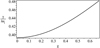 |
Fig. 3. Dependence of γ/lω1 on χ given by Eq. (106). |
| In the text | |
Current usage metrics show cumulative count of Article Views (full-text article views including HTML views, PDF and ePub downloads, according to the available data) and Abstracts Views on Vision4Press platform.
Data correspond to usage on the plateform after 2015. The current usage metrics is available 48-96 hours after online publication and is updated daily on week days.
Initial download of the metrics may take a while.