| Issue |
A&A
Volume 625, May 2019
|
|
|---|---|---|
| Article Number | A59 | |
| Number of page(s) | 9 | |
| Section | Planets and planetary systems | |
| DOI | https://doi.org/10.1051/0004-6361/201834368 | |
| Published online | 10 May 2019 | |
Constraining the orbit of the planet-hosting binary τ Boötis
Clues about planetary formation and migration★
Stellar Astrophysics Centre, Department of Physics and Astronomy, Aarhus University,
Ny Munkegade 120,
8000
Aarhus C,
Denmark
e-mail: justesen@phys.au.dk
Received:
3
October
2018
Accepted:
13
December
2018
Context. The formation of planets in compact or highly eccentric binaries and the migration of hot Jupiters are two outstanding problems in planet formation. Detailed characterisation of known systems is important for informing and testing models. The hot Jupiter τ Boo Ab orbits the primary star in the long-period (P ≳ 1000 yr), highly eccentric (e ~ 0.9) double star system τ Boötis. Due to the long orbital period, the orbit of the stellar binary is poorly constrained.
Aims. Here we aim to constrain the orbit of the stellar binary τ Boo AB in order to investigate the formation and migration history of the system. The mutual orbital inclination of the stellar companion and the hot Jupiter has important implications for planet migration. The binary eccentricity and periastron distance are important for understanding the conditions under which τ Boo Ab formed.
Methods. We combine more than 150 yr of astrometric data with twenty-five years of high-precision radial velocities. The combination of sky-projected and line-of-sight measurements places tight constraints on the orbital inclination, eccentricity, and periastron distance of τ Boo AB.
Results. We determine the orbit of τ Boo B and find an orbital inclination of 47.2−3.7+2.7°, a periastron distance of 28.3−3.0+2.3 au, and an eccentricity of 0.87−0.03+0.04. We find that the orbital inclinations of τ Boo Ab and τ Boo B, as well as the stellar spin-axis of τ Boo A coincide at ~45°, a result consistent with the assumption of a well-aligned, coplanar system.
Conclusions. The likely aligned, coplanar configuration suggests planetary migration within a well-aligned protoplanetary disc. Due to the high eccentricity and small periastron distance of τ Boo B, the protoplanetary disc was tidally truncated at ≈6 au. We suggest that τ Boo Ab formed near the edge of the truncated disc and migrated inwards with high eccentricity due to spiral waves generated by the stellar companion.
Key words: stars: individual: τ Boötis / planetary systems / planet-disk interactions / astrometry / techniques: radial velocities / planets and satellites: dynamical evolution and stability
Tables of the astrometric and radial velocity data are only available at the CDS via anonymous ftp to cdsarc.u-strasbg.fr (130.79.128.5) or via http://cdsarc.u-strasbg.fr/viz-bin/qcat?J/A+A/625/A59
© ESO 2019
1 Introduction
The origin of hot Jupiters is one of the longest-standing puzzles in exoplanetary science. The three most likely formation mechanisms – disc migration, high eccentricity migration, and in situ formation – all have theoretical and observational shortcomings (see Dawson & Johnson 2018 for a recent review). High-e migration theories propose migration triggered by dynamical interactions such as planet–planet scattering or Kozai–Lidov oscillations with subsequent tidal circulation (e.g. Weidenschilling & Marzari 1996; Wu & Murray 2003). During these interactions, the orbital eccentricity and inclination are excited to large values. High-e migration is motivated by measurements showing that a significant fraction of hot Jupiters orbiting F-type stars are misaligned with the spin-axis of their host stars (Winn et al. 2010; Albrecht et al. 2012a). For hot Jupiters orbiting binary (or multiple) stars, the stellar companion is a possible source of such interactions. One might expect that planets in compact or highly eccentric binaries (periastron distance aperi < 30 au) are likely candidates for having experienced this type of migration. However, the number of planets in such systems are expected to be limited due to star–disc interactions. The presence of a close stellar companion affects the protoplanetary disc, truncating the disc at a fraction of the periastron distance (Artymowicz & Lubow 1994). This effect reduces the disc mass and increases impact velocities within the disc, possibly inhibiting or preventing planet formation. Furthermore, discs in compact binaries show significantly reduced disc luminosities (i.e. masses) compared to single stars (Harris et al. 2012). For these reasons, it has been suggested that giant planets are unlikely to form in small-separation binaries (Jensen et al. 1996; Harris et al. 2012). Nevertheless, the discovery of several planetary systems in compact binaries shows that planets do form in such systems, contrary to expectations (e.g. γ Cephei A Hatzes et al. 2003 and Kepler-444A Dupuy et al. 2016). To understand the formation of planets in compact binaries, precise orbital parameters of both the planetary and stellar orbits are needed. In particular, the inclination, eccentricity, periastron distance, and mass ratio of the binary all impact the evolution of the disc as well as the formation and migration of planets in the system.
As a hot Jupiter orbiting an F-type star in an eccentric binary, τ Boo Ab is an ideal target for testing both hot Jupiter migration and planet formation in binaries. τ Boo is a bright (V = 4.5) planet-hosting double star. The binary contains the hot, massive star τ Boo A (F6V) orbited by the smaller companion τ Boo B (M2). τ Boo A hosts the hot Jupiter τ Boo Ab in a 3.3 day orbit (Butler et al. 1997). The stellar companion τ Boo B is in an eccentric, long-period orbit. The most recent estimates of the binary orbit are based on astrometric data and suggest a highly eccentric orbit e ~ 0.8 with a period of ~1000 yr (Roberts et al. 2011; Drummond 2014). Due to the long period, astrometric measurements cover less than 20% of the orbital period. Both Kozai–Lidov oscillations (Mede & Brandt 2014) and migration within an eccentricdisc (Roberts et al. 2011) have been suggested as possible migration mechanisms in the τ Boo system. However, the poorly constrained binary orbit has prevented any conclusive determination of the formation and migration scenario.
If the τ Boo system interacted dynamically and experienced high-e migration triggered by Kozai–Lidov oscillations, the planet and stellar companion are expected to orbit on mutually inclined orbits. If the planet and companion star migrated within an aligned disc, the system is expected to be coplanar. The orbital alignment between τ Boo Ab and τ Boo B is therefore crucial for understanding the formation of the system. Similarly, the eccentricity and periastron distance of τ Boo B determine the size of the protoplanetary disc in which τ Boo Ab formed.
We investigate the possible formation and migration mechanisms of the τ Boo system by precisely characterising the orbit of the τ Boo AB binary. This is achieved by combining more than 150 yr of astrometric data with 20 yr of high-precision radial velocities.
2 The τ Boo system
As a bright (V = 4.5) visual double star, τ Boo AB has been recognised as a stellar binary and has been measured astrometrically since 1825. Several authors have provided orbits for τ Boo B based on these astrometric data. The earliest orbital solutions were provided by Hale (1994) and Popović & Pavlović (1996) who found very different solutions of P = 2000 yr, e = 0.91 and P = 389 yr, e = 0.42, respectively. Recently, orbital solutions by Roberts et al. (2011) and Drummond (2014) find τ Boo B in a highly eccentric orbit (e = 0.76–0.84), with a period of ~ 1000 yr. These solutions predict a periastron passage between 2025 and 2035. Borsa et al. (2015) determined an eccentricity of e = 0.7 ± 0.2 by fitting radial velocities while fixing the period and periastron passage using the astrometric values from Drummond (2014). The primary component τ Boo A (F6V) has been studied extensively for signs of star–planet interactions due to its extremely rapid magnetic cycle of 240 days and likely tidally locked rotation (Shkolnik et al. 2005, 2008; Walker et al. 2008; Lanza 2009, 2012; Vidotto et al. 2012; Poppenhaeger & Wolk 2014; Borsa et al. 2015; Jeffers et al. 2018). Measurements of the magnetic field and S-index have revealed differential rotation on the order of ~ 20%. Mengel et al. (2016) measured the stellar rotation period using spectropolarimetric observations from 2011 to 2015 and report an equatorial angular velocity in the range Ωeq = 1.95–2.05 rad d−1, corresponding to rotation periods in the range P* = 3.06–3.34 days. At a stellar latitude of 40°, the stellar rotation period corresponds to the 3.3-day orbital period of τ Boo Ab, which suggests that tidal forces have forced the thin convective envelope of τ Boo A into corotation (Fares et al. 2009). Borsa et al. (2015) detected solar-like oscillations in τ Boo A and confirmed the strong differential rotation. We adopt the stellar parameters of τ Boo A by Valenti & Fischer (2005). The adopted stellar parameters of τ Boo A are listed in Table 1.
τ Boo Ab was discovered by Butler et al. (1997) via the radial-velocity method as part of the Lick planet search effort using the Hamilton spectrograph at the Lick observatory. τ Boo Ab is a non-transiting hot Jupiter in a 3.3-day orbit. As one of the earliest known and brightest exoplanetary systems, τ Boo Ab is one of the most well-studied exoplanets. The presence of CO (Brogi et al. 2012; Rodler et al. 2012)and water (Lockwood et al. 2014) has been measured in the absorption spectrum of τ Boo Ab using near-IR spectroscopy. These measurements have enabled the determination of the orbital inclination angle of τ Boo Ab. Brogi et al. (2012) and Rodler et al. (2012) determined an orbital inclination of iAb = 44.5 ± 1.5° and  respectively, by tracing the radial velocity shift of planetary CO absorption lines in the near-IR spectrum of τ Boo Ab. Lockwood et al. (2014) determined an orbital inclination of
  deg for τ Boo Ab by measuring the radial-velocity shift of water vapour in its atmosphere. For this study, we adopt the orbital inclination by Brogi et al. (2012). Knowledge of the orbital inclination has enabled the determination of the mass of τ Boo Ab at MAb = 5.95 ± 0.28MJup (Brogi et al. 2012). Also, τ Boo Ab has been the target of several searches for reflected light with a current 3σ upper-limit of the planet-to-star contrast of 1.5 × 10⁻⁵, corresponding to an optical albedo of 0.12 (Hoeijmakers et al. 2018).
Spectral type, magnitude, coordinates, parallax, proper motion, and stellar parameters of τ Boo A.
3 Observational data
We collect 192 yr of astrometric data from the Washington Double Star Catalog (WDS, Mason et al. 2001). The WDS contains 63 observations of τ Boo spanning the period 1825–2017. The three earliest measures, observed by J.F.W. Herschel between 1825 and 1831 (Herschel 1826, 1833, 1871) are outliers and are not used in the analysis. The second Gaia data release (DR2) contains the positions of τ Boo A and B (Gaia Collaboration 2016, 2018). From the Gaia DR2 positions, we compute a separation and position angle of (ρ, θ) = (1.662 ± 0.002′′, 67.36 ± 0.07°) at epoch 2015.5. This leaves us with an astrometric baseline of 168 yr including 61 observations from 1849 to 2017. We show the astrometric data (along with a model; see Sect. 5) in Fig. 1. The sky-projected position of τ Boo B has changedsignificantly in the past 200 yr. Astrometric data from the past two decades show the sky-projected separation approaching a minimum and a rapidly changing position angle, indicating that τ Boo B is close to periastron passage.
We use radial velocities from the Lick Planet Search program (Fischer et al. 2014). The survey was conducted from 1987 to 2011 using the Hamilton spectrograph at the Lick Observatory. τ Boo was continuously observed for the duration of the survey. We exclude data prior to 1995, which were taken with a separate setup and feature significantly more scatter than data gathered thereafter. The remaining Lick dataset contains 147 radial velocities taken from 1995 to 2011 with three instrumental setups. We furthermore include publicly available data from the GAPS programme using the HARPS-N spectrograph at the Telescopio Nazionale Galileo (TNG). Under this programme, τ Boo was observed on 12 nights between April 13 and May 14 2013 and on 11 nights between April 3 and July 22 2014 (Borsa et al. 2015). The GAPS data were obtained as part of an asteroseismic investigation and are therefore of high cadence with up to 30 spectra per night. We bin the GAPS data and use the median of each night. Finally, we observed τ Boo using HARPS-N on two nights, April 9 and July 4 2017. In total, we use 172 radial velocities spanning 22 yr.
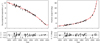 |
Fig. 1 Sky-projected separation (left) and position angle (right) of τ Boo over the past 168 yr. The median model from our MCMC analysis is plotted in red. From the rapidly shrinking separation and accelerating position angle, it is clear that τ Boo B is approaching periastron. Only a small arc of the full orbit is traced by these data. |
4 Analysis
4.1 Orbital model
We construct a Keplerian model to simultaneously fit radial velocities and astrometric data. To solve the 3D orbit, we use the equations of Keplerian motion. The 3D coordinates of the orbit may be expressed as (see e.g. Murray & Correia 2010)
![\begin{align}x &= r\left(\cos\Omega \cos (\omega + \nu) - \sin \Omega \sin (\omega + \nu) \cos i \right)\!, \\[1pt] y &= r\left(\sin\Omega \cos (\omega + \nu) + \cos \Omega \sin (\omega + \nu) \cos i \right)\!, \\[1pt] z &= r \sin(\omega + \nu)\sin i, \end{align}](/articles/aa/full_html/2019/05/aa34368-18/aa34368-18-eq6.png)
where  , a is the semi-major axis, Ω is the longitude of the ascending node, ω is the argument of periastron, i is orbital inclination, (x, y) are the sky-projected coordinates, and z is the line-of-sight coordinate. The sky-projected coordinates (x, y) are converted into the astrometric observables (projected separation ρ and positionangle θ) via

The astrometric data measure the apparent size of the orbit on the sky. To compute the physical size of the orbit, we scale the orbit by the stellar distance d = 1∕π, using the parallax π. Radial velocity data help to further constrain the orbital parameters. The line-of-sight velocity is computed as
 (6)
(6)
where γi is a velocity offset and K is the radial velocity semi-amplitude, which is a function of the masses M1 and M2, the inclination i, the semi-major axis a and eccentricity e. In summary, to fit radial velocities and astrometric observables of an orbit, our model requires the parameters (a, T0, e, ω, Ω, i, M1, M2, d, γ).
4.2 Comparing model to data
The astrometric measurements in the WDS are sourced from different observers using different instrumental setups over a period of more than 150 yr. The measurements prior to 1998 are almost exclusively made with micrometers on photographic plates. Only data collected after 1998 have formal uncertainties listed1. To ensure a proper weighting of the data we fit error terms σρ,pre 1998 and σθ,pre 1998 to astrometric data taken prior to 1998. The formal uncertainties on the post-1998 astrometric data ranges from 0.002 to 0.04′′ in separation and 0.07 to 1.0° in position angle. To account for potential systematic uncertainties (due to instrumental and atmospheric effects) we fit jitter error terms σρ,post 1998 and σθ,post 1998 to this data.
Similarly, the radial velocities are obtained using different instrumental setups. The Lick data have a mean uncertainty of 8 m s−1, while the HARPS-N data have a meanuncertainty of 1 m s−1. Due to intrinsic instrumental effects, atmospheric conditions and stellar variability, these uncertainties do not reflect the true error of the measurements. Using the high-cadence GAPS data, Borsa et al. (2015) found peak-to-peak variations of up to 15 m s−1 with typical variability less than 10 m s−1. To account for this additional noise, we include a jitter term σRV, i for each instrumental setup. In order to combine the four radial velocity datasets, we include four velocity offsets γi.
The orbits of the stellar companion τ Boo B and the hot Jupiter τ Boo Ab are fitted simultaneously. The astrometric reflex motion of τ Boo A due to the planet τ Boo Ab is of the order of ~10 μas, roughly three orders of magnitude smaller than the estimated astrometric uncertainties. We therefore neglect the astrometric signal of the planet. Butler et al. (1997) reported a marginal eccentricity of τ Boo Ab at the 1σ level. Brogi et al. (2012) redetermined the orbit and found that when excluding noisy Lick data prior to 1995, an eccentric solution is no longer preferred. Borsa et al. (2015), also excluding early Lick data, determined a small eccentricity of 0.011 at the 2σ level with an argument of periastron near 90°. However, eccentricities derived from radial velocities may be biased towards larger values (Zakamska et al. 2011). In particular, the combination of a small eccentricity and an argument of periastron close to 90° is indicative of a potential observational bias (Albrecht et al. 2012b). We therefore adopt a circular orbit of τ Boo Ab. By neglecting the astrometric contribution and adopting a circular orbit, we reduce the dimensionality by four parameters. For τ Boo B we include the full astrometric and radial velocity signal. The final model contains 24 parameters (listed in Table 2): six parameters describing the orbit of τ Boo B, three parameters describing the orbit of τ Boo Ab, four velocity offsets, four radial velocity jitter terms, four astrometric error terms, the stellar masses of τ Boo A and B, and finally the distance. We adopt the joint log-likelihood function
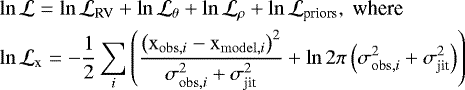 (7)
(7)
and  is the combined log-likelihood of the priors described below. We impose Gaussian priors on the primary stellar mass MA and distance d (using the values in Table 1). We impose a sin i prior on theinclination, appropriate for an isotropic orientation. We use a log-normal prior with a mean of log10(P∕days) = 5.03 and a standard deviation of
  2.28 on the period of the binary, consistent with the period distribution of binaries determined by Raghavan et al. (2010). For the remaining parameters we assume uniform priors. We sample the posterior distribution using the affine invariant MCMC ensemble sampler emcee (Foreman-Mackey et al. 2013).
We run the MCMC algorithm for 3.6 × 10⁶ iterations using 96 parallel chains for a total of 346 × 106 samples. We reject the initial 1.2 × 10⁶ steps of each chain and thin by a factor of six.
Parameters of the τ Boo system.
5 Results
The results of the analysis are listed in Table 2. We report median values with 1σ (16 and 84% quantile) uncertainties. The median model is plotted in Fig. 1 along with the astrometric data and residuals, and in Fig. 2 with radial velocities and residuals. In Fig. 3, the sky-projected orbit and radial velocity curve are plotted with the median and 100 orbits drawn from the posterior. τ Boo B is in a highly eccentric (e = ) orbit. As evident from the rapidly shrinking separation and the significant change in the radial velocity amplitude in the past 25 yr, τ Boo AB is rapidly approaching periastron. We predict periastron in the year
  . The period (P =
  yr) and semi-major axis (a =
  au) are relatively poorly determined. This is a general feature of orbits with low orbital coverage, since it is possible to draw an almost arbitrarily large ellipse through the data. However, the data close to periastron passage enable a precise determination of the periastron distance of
  au. The combination of astrometry and radial velocity constrains the 3D orientation of the orbit, allowing us to derive Ω =
  °, ω =
  °, and i =
  °. While the period and semi-major axis are relatively poorly constrained, the relation
  1.84 ± 0.03, equivalent to the mass sum in solar units via Kepler’s third law, is much more precise. This was noted by Eggen (1967) who discovered that is it possible to derive reliable mass sums even for binaries with low orbital coverage. Combining the mass sum with the mass of τ Boo A (MA = 1.35 ± 0.03 M⊙) we get a precise mass of τ Boo B MB = 0.49 ± 0.02 M⊙. Assuming that the two stellar companions have the same age and metallicity, we determine the radius of τ Boo B by fitting the age, metallicity and mass to a grid of BaSTI isochrones (Pietrinferni et al. 2004) using the BAyesian STellar Algorithm, BASTA (Silva Aguirre et al. 2015). We find Teff, B = 3580 ± 90 K and RB = 0.48 ± 0.05 R⊙. The effective temperature is in good agreement with the temperature Teff, B = 3425 ± 100 K determined by Lindgren et al. (2016) using high-resolution IR spectroscopy.
As a consistency check of our solution, we check that the change in proper motion (i.e. sky-projected velocity) of τ Boo A between HIPPARCOS and Gaia DR2 is consistent with the change expected from our solution. We predict a change in the proper motion of τ Boo A due to its astrometric reflex motion caused by τ Boo B. We note that the proper motions reported by HIPPARCOS and Gaia DR2 are derived by assuming a constant proper motion for the duration of their observations. This assumption does not hold for τ Boo A, since the magnitude of its proper motion changes by ~ 1.6 mas yr−1 during Gaia DR2 observations and ~ 1.2 mas yr−1 during HIPPARCOS observations. The HIPPARCOS and Gaia DR2 measurements are therefore likely not as accurate as the reported formal uncertainties suggest. To compare with our model, we compute the mean proper motion of τ Boo A over the observing periods of HIPPARCOS (1989.8–1993.2) and Gaia DR2 (2014.6–2016.4). From our analysis, we find that the magnitude and angle of the proper motion difference Δμ of τ Boo A are  mas yr−1 at an angle θ = arctan(Δμα∕Δμδ) = 47.6 ± 2.4°. The magnitude and angle of the proper motion difference between the HIPPARCOS and Gaia DR2 catalogues are Δμ = 16.1 ± 0.9 mas yr−1 and θ = 46.0 ± 2.3°, in good agreement with our solution.
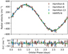 |
Fig. 2 Phase-folded radial velocity curve of τ Boo A without the contribution from τ Boo B. The median model is plotted in black. |
6 Discussion
6.1 Mutual inclinations in the τ Boo system
The orbital inclination of the stellar companion τ Boo B is important for understanding the dynamical evolution of the τ Boo system. If the stellar companion triggered the migration of the hot Jupiter τ Boo Ab via the Kozai–Lidov mechanism, τ Boo Ab and τ Boo B are expected to orbit on mutually inclined orbits. In classic Kozai–Lidov theory, the minimum mutual inclination required to excite an eccentricity emax is (Holman et al. 1997)
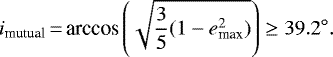 (8)
(8)
From the joint astrometric and radial velocity analysis we determine an orbital inclination of τ Boo B of iB =  °. This value is consistent with the orbital inclination of τ Boo Ab (iAb = 44.5 ± 1.5°), suggesting a coplanar configuration with at most a small mutual inclination
  . The mutual inclination is too small to have triggered Kozai–Lidov oscillations. To investigate the spin-orbit alignment, we determine the inclination angle of the stellar spin-axis of τ Boo A by combining the stellar radius, rotation period, and projected rotational velocity (as given in Table 1)
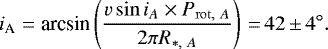 (9)
(9)
We find that all three inclination angles agree within their uncertainties. The probability density functions of the three inclination angles are plotted in Fig. 4. The three coinciding inclination angles are consistent with the assumption of a flat system architecture in which the orbits of the companions τ Boo Ab and τ Boo B are both aligned within a few degrees of the stellar spin-axis of τ Boo A. We note that the inclination angles measure only the projected alignment along the line of sight. The longitude of the ascending node of the orbit of τ Boo Ab, as well as the sky-projection of the stellarspin-axis of τ Boo A are unconstrained by the data. Since the sky-projected alignment is unconstrained, it is possible that the system is non-coplanar and misaligned in 3D space. It is however unlikely that all three inclination angles would agree by coincidence. The assumption of coplanarity and alignment is the simplest (but not the only) interpretation of the data. In the following section we therefore assume that the system is coplanar and aligned and discuss the implications of this assumption.
It is unlikely that tidal forces have realigned the orbits or spin-axis in the system. If τ Boo Ab has been tidally realigned with the stellar spin-axis, we would not expect the stellar spin-axis to be aligned with the outer companion. Additionally, due to its shallow convective envelope, the tidal forces of τ Boo A are expected to be too weak to realign a misaligned orbit. Using the calibrated timescale for changing the spin of a star from Hansen (2012) and assuming a stellar gyration radius  , a stellar dissipation coefficient
  (appropriate for a 1.35 M⊙ star) and a planet radius of 1.15 RJup, we find a timescale of Tspin ~ 1011 yr, much longer than the ~1 Gyr age of the τ Boo system. We therefore conclude that both τ Boo Ab and τ Boo B formed and migrated within a primordially aligned disc. Using Eq. (1) in Holman & Wiegert (1999)2, we find that planetary orbits in the τ Boo AB binary are stable out to 2% of the binary semi-major axis, a condition easily satisfied by τ Boo Ab which orbits at a distance of less than 0.05% of the binary semi-major axis.
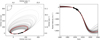 |
Fig. 3 Left panel: sky-projected relative orbit of τ Boo AB in apparent size (′′) and absolute size (au). See Fig. 1 for a closer view of the astrometric data and model residuals. Right panel: radial velocity curve of τ Boo A with planetary radial velocity signal subtracted. See Fig. 2 for a closer view of the radial velocity curve and model residuals. |
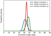 |
Fig. 4 Probability density of the inclination of the stellar spin-axis of τ Boo A iA (derived from v sin i, R* and Prot, see Table 1), the orbital inclination angle of τ Boo Ab iAb (determined via the planetary radial velocity signal by Brogi et al. 2012) and the orbital inclination angle of τ Boo B iAB (determined from our MCMC analysis). The similarity of the three inclination angles suggests a coplanar, aligned system. |
6.2 Truncation of the protoplanetary disc
The formation of circumstellar (S-type) planets around close or highly eccentric binaries presents a significant challenge for current formation theories. In a close binary, the protoplanetary disc around the primary star will be tidally truncated by the companion at a fraction of the periastron distance (Artymowicz & Lubow 1994). The location of the truncation radius depends on the separation, mass ratio, eccentricity, and inclination of the companion.
Due to the high eccentricity of τ Boo B, the periastron approach may be approximated as a parabolic stellar fly-by. Clarke & Pringle (1993) studied the influence of a single coplanar fly-by and found that the disc is typically stripped of material down to ≈ 0.5aperi. Breslau et al. (2014), also studying stellar fly-bys, found a simple relation atrunc = 0.28μ−0.32aperi ≈ 0.4aperi between the truncated disc size atrunc and the mass-ratio μ and periastron distance aperi of the fly-by. Bhandare et al. (2016) showed that inclined encounters truncate the protoplanetary disc slightly less efficiently than coplanar encounters, with an approximately linearly decreasing effect on final disc size with increasing star-disc inclination. It is clear that even a single encounter truncates the disc at a fraction of the periastron distance.
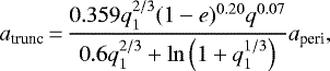
Pichardo et al. (2005) studied the discs of stars in binaries by simulating the effect of periodic gravitational perturbations on test-particle orbits. From their numerical simulations they derive an equation estimating the outer truncation radius of circumstellar discs in binaries:
 (10)
(10)
where q = m2∕(m1 + m2) and q1 = (1 − q)∕q. For τ Boo A, we find a truncation radius of atrunc ≈ 0.2aperi ≈ 6 au. This truncation radius is a factor of two smaller than the expected truncation radius caused by a single stellar encounter.
6.3 Planet formation and migration in a truncated disc
Not only is the protoplanetary disc truncated, the shape and velocity dispersion of the disc are also affected. The increased velocity dispersion in a perturbed disc may prohibit planetesimal growth. Kobayashi & Ida (2001) studied the velocity dispersion of planetesimals in a circular disc after a stellar encounter and find that planet formation is inhibited in the outer disc due to increased relative impact velocities. They derive the outer boundary of the planet-forming radius aplanet as the distance below which the velocity dispersion is low enough for planet formation. They find the relation
 (11)
(11)
where μ = m1∕m2. The estimated outer radius of the planet-forming region is comparable to the truncation radius, suggesting that planet formation is possible in the truncated disc. The eccentricity of the disc is another problem for efficient planet formation. In an eccentric disc, relative impact velocities are increased, impeding (or potentially preventing) grain accumulation (Thébault et al. 2006). However, simulations show that disc self-gravitation acts to reduce relative impact velocities and may enable planetesimal growth in binaries with massive discs (Marzari et al. 2009; Rafikov 2013). Marzari et al. (2009) and Regály et al. (2011) found that circumstellar disc eccentricity decreases for increasing binary eccentricity. The conditions for planet formation may therefore be more favourable in eccentric binaries than in compact circular binaries.
Kley & Nelson (2008) studied the migration of protocores in the circumstellar disc of γ Cephei A, which is the primary component of an eccentric binary (a = 18.5 au, MA = 1.59 M⊙, MB = 0.38 M⊙, e = 0.36) hosting a a = 2.1 au, m sin i = 1.7 MJup planet in a coplanar configuration (Hatzes et al. 2003). Their simulations show that perturbations from γ Cephei B periodically generate strong spiral waves propagating towards the centre of the circumstellar disc around γ Cephei A. They found that gas accretion in such a system is efficient, with a 3 MJup disc being sufficient to create a 2 MJup planet. Embedded protocores initially placed within a < 2.7 au migrate inwards with limited eccentricities, while cores placed at larger distances acquire large eccentricities while slowlymigrating inwards. The location of this transition boundary depends on disc mass, viscosity, and temperature. Rafikov & Silsbee (2015) similarly found that is it possible to form giant planets at au-scale orbits in ~ 20 au-separation eccentric binaries given that the disc is massive and nearly circular.
There is some observational evidence that companion stars excite spiral arms in protoplanetary discs. The protoplanetary disc around HD 100453A features a two-armed spiral structure (Wagner et al. 2015). Dong et al. (2016) and Wagner et al. (2018) found that the observed spiral arm structure is most likely generated by the mildly eccentric coplanar stellar companion at a separation of ~ 120 au. The stellar companion has truncated the disc of HD 100453A at ~40 au, in good agreement with the numerical simulations discussed earlier. Ngo et al. (2016) found that while hot-Jupiter host stars have a companion fraction in the range 50–2000 au that is approximately three times larger than that of field stars, the stellar companions are unlikely to cause Kozai–Lidov migration. This suggests that some other mechanism produces hot Jupiters in these binaries.
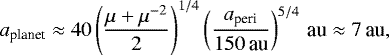
Spiral density wave-induced disc migration may explain the presence of hot Jupiters in binary stars with small periastron distances. In this picture, a protocore forms at the ice line near the outer edge of the truncated disc and acquires a large eccentricity while efficiently accreting gas until being tidally circularized in a short-period orbit. Density wave-induced spiral arms in the disc generated by the stellar companion facilitate both the formation of the protocore (due to increased surface density in the spiral arms) and trigger inwards disc migration, either eccentric or circular depending on where in the disc the core forms. Core formation is typically most efficient just outside the ice line. Inside the ice line, gases cannot condense into grains needed for efficient core growth3. At large distances core accretion is too slow. The location of the ice line of τ Boo A is estimated as (Ida & Lin 2005)
 (12)
(12)
The location of the ice line is comparable to the estimated planet-forming region and the disc truncation radius, indicating that planet formation occurs near the disc edge. The high-density spiral arms may offer favourable conditions for rapid core growth. Core growth by for example pebble accretion depends strongly on metallicity and surface density (Lambrechts & Johansen 2014). The high metallicity of τ Boo A ([Fe/H] = 0.25 dex) enables rapid assembly of the protocore, which is needed in order for the protocore to accrete enough gas before the disc disperses. A scenario in which the massive planet formed near 5 au and migrated inwards is consistent with the predictions from pebble accretion (Bitsch et al. 2015).
Assuming an accretion efficiency similar to γ Cephei A, a disc mass of at least ≈ 8 MJup is required to form a massive hot Jupiter such as τ Boo Ab (at 6 MJup). This requires a disc-to-star mass ratio of Md∕M*≈ 0.5% of the truncated disc. Andrews et al. (2013) report typical values of Md ∕M*≈ 0.2–0.6% for single stars with full discs but with a distribution reaching Md∕M*≈ 10% at the highest end. If τ Boo A had an initially massive disc of 0.1 M*≈ 140 MJup, the disc could have lost 95% of its mass while still providing sufficient material for the formation of τ Boo Ab. However, the luminosity of discs around components in binaries with separations < 300 au are typically reduced by a factor of five compared to single stars (Jensen et al. 1994, 1996; Harris et al. 2012), suggesting that massive discs are uncommon in compact binaries.
If spiralwave-induced disc migration is a dominant source of hot Jupiters in stellar binaries, we expect that hot Jupiters in binary systems are tracers of primordial disc alignment. Hot Jupiters born in binaries with aligned discs are therefore expected to be spin-orbit aligned. However, protoplanetary discs in binary systems are not always well-aligned. The protoplantary discs in the young binary HK Tauri are misaligned by ~ 60°, indicating that one or both discs are misaligned with the binary orbit (Jensen & Akeson 2014). The protoplanetary discs in the binary protostar IRS 43 are similarly misaligned with respect to the binary plane (Brinch et al. 2016). An inclined binary companion may cause the primary protoplanetary disc to precess and eventually become misaligned with the stellar spin-axis (Batygin 2012; Lai 2014). Tokovinin (2017) found strong orbital alignment in triple star systems with outer projected separations less than ~ 50 au and misalignment in systems with outer orbits wider than 1000 au. Hale (1994) similarly found spin-orbit alignment in binaries with separations less than 30–40 au. This suggests that hot Jupiters in compact binaries are more likely to be spin-orbit aligned. The Catalog of Exoplanets in Binary Star Systems4 (Schwarz et al. 2016) lists 13 planet-hosting binaries with projected separations less than 50 au. Out of these 13 systems5, only WASP-11Ab (with a separation of 42 au) has a measured projected spin-orbit alignment of λ = 7 ± 5° (Mancini et al. 2015). WASP-11Ab likely formed in a truncated disc similar to τ Boo Ab. However, we note that due to its low effective temperature (Teff = 4900 ± 65 K), tidal forces could have realigned the stellar spin-axis of WASP-11A. The Transiting Exoplanet Survey Satellite (TESS) started science operations on July 25 2018 and will complete a near all-sky survey in two years (Ricker et al. 2015). TESS will increase the number of bright planets amenable for follow-up observations and will likely expand the sample of known planets in compact binaries.
Due to the challenges of forming planets in discs around close binaries, several alternative formation scenarios have been proposed. Gong & Ji (2018) investigated the conversion of a P-to-S-type planet by scattering-induced capture. In this scenario, a circumbinary planet in a close (a = 0.5–3 au) binary is dynamically scattered before being tidally captured by the primary or secondary star. However, the probability of such an event is highest for small mass ratios and compact, nearly circular binaries. This scenario is therefore unlikely to provide a formation path for τ Boo Ab. Another possibility is that the current configuration of the binary is different from the configuration at planet formation. If the binary was less eccentric at the time of planet formation, the protoplanetary disc of τ Boo A would have lost less mass and the formation of massive planets would have been more favourable. Marzari & Barbieri (2007) studied the orbital evolution of binary stars due to stellar encounters and found that a single stellar encounter may significantly change the orbit of a binary without ejecting planets. However, such an encounter will typically alter the inclination of the binary orbit. The aligned, coplanar configuration of the τ Boo system suggests that it has not been subject to external perturbations or three-body interactions since formation. Furthermore, the probability of a sufficiently close stellar encounter is extremely small for field stars. Another possibility is that the eccentricity of τ Boo B has been raised by star–disc interactions after or during formation of the planet. Artymowicz et al. (1991) found that star–disc interactions rapidly excite the eccentricity of proto-binaries while in the embedded disc phase. The growth of binary eccentricity occurs before disc dispersal. The eccentricity of τ Boo B is therefore unlikely to have changed significantly after dispersal of the disc.
The combination of astrometry and radial velocities is a powerful method for constraining 3D orbits. When Gaia epoch astrometry is released it will be possible to fit the relative motion of τ Boo A and B and similar binaries. This will help to further constrain the orbits of long-period binaries. The Gaia mission is expected to discover tens of thousands of planets based on high-precision astrometric measurements (Perryman et al. 2014). By combining Gaia astrometry with radial velocities, it will become possible to obtain 3D solutions of binary star and exoplanet orbits. This will be a valuable tool for breaking the degeneracy between the projected orbital alignment and the true 3D alignment in multi-planet systems and planet-hosting binaries.
7 Conclusions
By determining the inclination, eccentricity, and periastron distance of τ Boo B we find an orbital architecture of the τ Boo system consistent with the assumption of an aligned, coplanar configuration. This configuration suggests that we are observing the primordial configuration of the system and that dynamical interactions such as the Kozai–Lidov mechanism have not played a role in this system. We suggest a likely formation pathway for τ Boo Ab and similar hot Jupiters: The stellar companion (with a periastron distance of ~ 30 au) truncated the protoplanetary disc of τ Boo A near the ice line, reducing the disc to a fraction of its initial size. τ Boo Ab likely formed near the outer edge of this truncated disc and migrated inwards in the disc due to spiral waves generated by the eccentric stellar companion. During migration, τ Boo Ab acquired a large eccentricity that was tidally dampened by τ Boo A, creating the hot Jupiter we observe today. This scenario requires an initially massive protoplanetary disc, rapid assembly of the protocore and highly efficient gas accretion. The existence of planets in compact and eccentric binaries such as τ Boo and γ Cephei proves that giant planet formation is possible even in these challenging environments. The discovery and characterisation of the orbital architecture of planet-hosting binaries such as τ Boo are crucial for informing models of planet formation and migration.
Acknowledgements
We thank Davide Gandolfi and Artie Hatzes for the time exchange that made our HARPS-N observations possible. Wethank Anders Johansen for discussions that improved this article. We thank the anonymous referee for quick and useful comments that improved the clarity of the manuscript. We acknowledge support from the Danish Council for Independent Research, through a DFF Sapere Aude Starting Grant no. 4181-00487B. Funding for the Stellar Astrophysics Centre is provided by The Danish National Research Foundation (Grant agreement no.: DNRF106). Based on observations made as part of the observing programs OPT17A_64 and A35TAC_26 with the Italian Telescopio Nazionale Galileo (TNG) operated on the island of La Palma by the Fundación Galileo Galilei of the INAF (Istituto Nazionale diAstrofisica) at the Spanish Observatorio del Roque de los Muchachos of the Instituto de Astrofisica de Canarias. This projecthas received funding from the European Union’s Horizon 2020 research and innovation programme under grant agreement No 730890. This material reflects only the authors views and the Commission is not liable for any use that may be made of the information contained therein. This research has made use of the Washington Double Star Catalog maintained at the U.S. Naval Observatory. This work has made use of data from the European Space Agency (ESA) mission Gaia (https://www.cosmos.esa.int/gaia), processed by the Gaia Data Processing and Analysis Consortium (DPAC, https://www.cosmos.esa.int/web/gaia/dpac/consortium). Funding for the DPAC has been provided by national institutions, in particular the institutions participating in the Gaia Multilateral Agreement. This research made use of NumPy (Van Der Walt et al. 2011), SciPy (Jones et al. 2001) and corner.py (Foreman-Mackey 2016). This research made use of Astropy, a community-developed core Python package for Astronomy (Astropy Collaboration 2018). This research made use of matplotlib, a Python library for publication quality graphics (Hunter 2007). This research has made use of the SIMBAD database, operated at CDS, Strasbourg, France (Wenger et al. 2000). This research has made use of NASA’s Astrophysics Data System.
References
- Albrecht, S., Winn, J. N., Johnson, J. A., et al. 2012a, ApJ, 757, 18 [NASA ADS] [CrossRef] [Google Scholar]
- Albrecht, S., Winn, J. N., Butler, R. P., et al. 2012b, ApJ, 744, 189 [NASA ADS] [CrossRef] [Google Scholar]
- Andrews, S. M., Rosenfeld, K. A., Kraus, A. L., & Wilner, D. J. 2013, ApJ, 771, 129 [NASA ADS] [CrossRef] [Google Scholar]
- Artymowicz, P., & Lubow, S. H. 1994, ApJ, 421, 651 [NASA ADS] [CrossRef] [Google Scholar]
- Artymowicz, P., Clarke, C. J., Lubow, S. H., & Pringle, J. E. 1991, ApJ, 370, L35 [NASA ADS] [CrossRef] [Google Scholar]
- Astropy Collaboration (Price-Whelan, A. M., et al.) 2018, AJ, 156, 123 [Google Scholar]
- Batygin, K. 2012, Nature, 491, 418 [NASA ADS] [CrossRef] [PubMed] [Google Scholar]
- Bhandare, A., Breslau, A., & Pfalzner, S. 2016, A&A, 594, A53 [NASA ADS] [CrossRef] [EDP Sciences] [Google Scholar]
- Bitsch, B., Lambrechts, M., & Johansen, A. 2015, A&A, 582, A112 [NASA ADS] [CrossRef] [EDP Sciences] [Google Scholar]
- Borsa, F., Scandariato, G., Rainer, M., et al. 2015, A&A, 578, A64 [NASA ADS] [CrossRef] [EDP Sciences] [Google Scholar]
- Breslau, A., Steinhausen, M., Vincke, K., & Pfalzner, S. 2014, A&A, 565, A130 [NASA ADS] [CrossRef] [EDP Sciences] [Google Scholar]
- Brinch, C., Jørgensen, J. K., Hogerheijde, M. R., Nelson, R. P., & Gressel, O. 2016, ApJ, 830, L16 [NASA ADS] [CrossRef] [Google Scholar]
- Brogi, M., Snellen, I. A. G., de Kok, R. J., et al. 2012, Nature, 486, 502 [NASA ADS] [CrossRef] [PubMed] [Google Scholar]
- Butler, R. P., Marcy, G. W., Williams, E., Hauser, H., & Shirts, P. 1997, ApJ, 474, L115 [NASA ADS] [CrossRef] [Google Scholar]
- Clarke, C. J., & Pringle, J. E. 1993, MNRAS, 261, 190 [NASA ADS] [CrossRef] [Google Scholar]
- Dawson, R. I., & Johnson, J. A. 2018, ARA&A, 56, 175 [NASA ADS] [CrossRef] [Google Scholar]
- Dong, R., Zhu, Z., Fung, J., et al. 2016, ApJ, 816, L12 [NASA ADS] [CrossRef] [Google Scholar]
- Drummond, J. D. 2014, AJ, 147, 65 [NASA ADS] [CrossRef] [Google Scholar]
- Dupuy, T. J., Kratter, K. M., Kraus, A. L., et al. 2016, ApJ, 817, 80 [NASA ADS] [CrossRef] [Google Scholar]
- Eggen, O. J. 1967, ARA&A, 5, 105 [NASA ADS] [CrossRef] [Google Scholar]
- Fares, R., Donati, J.-F., Moutou, C., et al. 2009, MNRAS, 398, 1383 [NASA ADS] [CrossRef] [MathSciNet] [Google Scholar]
- Fischer, D. A., Marcy, G. W., & Spronck, J. F. P. 2014, ApJS, 210, 5 [NASA ADS] [CrossRef] [Google Scholar]
- Foreman-Mackey, D. 2016, J. Open Source Softw., 1, 24 [Google Scholar]
- Foreman-Mackey, D., Hogg, D. W., Lang, D., & Goodman, J. 2013, PASP, 125, 306 [CrossRef] [Google Scholar]
- Gaia Collaboration (Prusti, T., et al.) 2016, A&A, 595, A1 [NASA ADS] [CrossRef] [EDP Sciences] [Google Scholar]
- Gaia Collaboration (Brown, A. G. A., et al.) 2018, A&A, 616, A1 [NASA ADS] [CrossRef] [EDP Sciences] [Google Scholar]
- Gong, Y.-X., & Ji, J. 2018, MNRAS, 478, 4565 [NASA ADS] [CrossRef] [Google Scholar]
- Hale, A. 1994, AJ, 107, 306 [NASA ADS] [CrossRef] [Google Scholar]
- Hansen, B. M. S. 2012, ApJ, 757, 6 [NASA ADS] [CrossRef] [Google Scholar]
- Harris, R. J., Andrews, S. M., Wilner, D. J., & Kraus, A. L. 2012, ApJ, 751, 115 [NASA ADS] [CrossRef] [Google Scholar]
- Hatzes, A. P., Cochran, W. D., Endl, M., et al. 2003, ApJ, 599, 1383 [NASA ADS] [CrossRef] [Google Scholar]
- Herschel, J. F. W. 1826, MNRAS, 2, 459 [NASA ADS] [Google Scholar]
- Herschel, J. F. W. 1833, MNRAS, 6, 1 [NASA ADS] [Google Scholar]
- Herschel, J. F. W. 1871, MNRAS, 38, 1 [NASA ADS] [Google Scholar]
- Hoeijmakers, H. J., Snellen, I. A. G., & van Terwisga, S. E. 2018, A&A, 610, A47 [NASA ADS] [CrossRef] [EDP Sciences] [Google Scholar]
- Holman, M. J., & Wiegert, P. A. 1999, AJ, 117, 621 [NASA ADS] [CrossRef] [Google Scholar]
- Holman, M., Touma, J., & Tremaine, S. 1997, Nature, 386, 254 [NASA ADS] [CrossRef] [Google Scholar]
- Hunter, J. D. 2007, Comput. Sci. Eng., 9, 90 [NASA ADS] [CrossRef] [Google Scholar]
- Ida, S., & Lin, D. N. C. 2004, ApJ, 604, 388 [NASA ADS] [CrossRef] [PubMed] [Google Scholar]
- Ida, S., & Lin, D. N. C. 2005, ApJ, 626, 1045 [NASA ADS] [CrossRef] [Google Scholar]
- Jeffers, S. V., Mengel, M., Moutou, C., et al. 2018, MNRAS, 479, 5266 [NASA ADS] [CrossRef] [Google Scholar]
- Jensen, E. L. N., & Akeson, R. 2014, Nature, 511, 567 [NASA ADS] [CrossRef] [Google Scholar]
- Jensen, E. L. N., Mathieu, R. D., & Fuller, G. A. 1994, ApJ, 429, L29 [NASA ADS] [CrossRef] [Google Scholar]
- Jensen, E. L. N., Mathieu, R. D., & Fuller, G. A. 1996, ApJ, 458, 312 [Google Scholar]
- Jones, E., Oliphant, T., Peterson, P., et al. 2001, SciPy: Open source scientific tools for Python [Google Scholar]
- Kley, W., & Nelson, R. P. 2008, A&A, 486, 617 [NASA ADS] [CrossRef] [EDP Sciences] [Google Scholar]
- Kobayashi, H., & Ida, S. 2001, Icarus, 153, 416 [NASA ADS] [CrossRef] [Google Scholar]
- Lai, D. 2014, MNRAS, 440, 3532 [NASA ADS] [CrossRef] [Google Scholar]
- Lambrechts, M., & Johansen, A. 2014, A&A, 572, A107 [NASA ADS] [CrossRef] [EDP Sciences] [Google Scholar]
- Lanza, A. F. 2009, A&A, 505, 339 [NASA ADS] [CrossRef] [EDP Sciences] [Google Scholar]
- Lanza, A. F. 2012, A&A, 544, A23 [NASA ADS] [CrossRef] [EDP Sciences] [Google Scholar]
- Lindgren, S., Heiter, U., & Seifahrt, A. 2016, A&A, 586, A100 [NASA ADS] [CrossRef] [EDP Sciences] [Google Scholar]
- Lockwood, A. C., Johnson, J. A., Bender, C. F., et al. 2014, ApJ, 783, L29 [NASA ADS] [CrossRef] [Google Scholar]
- Mancini, L., Esposito, M., Covino, E., et al. 2015, A&A, 579, A136 [NASA ADS] [CrossRef] [EDP Sciences] [Google Scholar]
- Marzari, F., & Barbieri, M. 2007, A&A, 467, 347 [NASA ADS] [CrossRef] [EDP Sciences] [Google Scholar]
- Marzari, F., Scholl, H., Thébault, P., & Baruteau, C. 2009, A&A, 508, 1493 [NASA ADS] [CrossRef] [EDP Sciences] [Google Scholar]
- Mason, B. D., Wycoff, G. L., Hartkopf, W. I., Douglass, G. G., & Worley, C. E. 2001, AJ, 122, 3466 [Google Scholar]
- Mede, K., & Brandt, T. D. 2014, Exploring the Formation and Evolution of Planetary Systems, eds. M. Booth, B. C. Matthews, & J. R. Graham, IAU Symp., 299, 52 [NASA ADS] [Google Scholar]
- Mengel, M. W., Fares, R., Marsden, S. C., et al. 2016, MNRAS, 459, 4325 [NASA ADS] [CrossRef] [Google Scholar]
- Murray, C. D., & Correia, A. C. M. 2010, Keplerian Orbits and Dynamics of Exoplanets (Tucson: University of Arizona Press), 15 [Google Scholar]
- Ngo, H., Knutson, H. A., Hinkley, S., et al. 2016, ApJ, 827, 8 [NASA ADS] [CrossRef] [Google Scholar]
- Perryman, M., Hartman, J., Bakos, G. Á., & Lindegren, L. 2014, ApJ, 797, 14 [NASA ADS] [CrossRef] [Google Scholar]
- Pichardo, B., Sparke, L. S., & Aguilar, L. A. 2005, MNRAS, 359, 521 [NASA ADS] [CrossRef] [Google Scholar]
- Pietrinferni, A., Cassisi, S., Salaris, M., & Castelli, F. 2004, ApJ, 612, 168 [NASA ADS] [CrossRef] [Google Scholar]
- Popović, G. M., & Pavlović, R. 1996, Bull. Astron. Belgrade, 153, 57 [NASA ADS] [Google Scholar]
- Poppenhaeger,K., & Wolk, S. J. 2014, A&A, 565, L1 [NASA ADS] [CrossRef] [EDP Sciences] [Google Scholar]
- Rafikov, R. R. 2013, ApJ, 765, L8 [NASA ADS] [CrossRef] [Google Scholar]
- Rafikov, R. R., & Silsbee, K. 2015, ApJ, 798, 70 [NASA ADS] [CrossRef] [Google Scholar]
- Raghavan, D., McAlister, H. A., Henry, T. J., et al. 2010, ApJS, 190, 1 [NASA ADS] [CrossRef] [EDP Sciences] [Google Scholar]
- Regály, Z., Sándor, Z., Dullemond, C. P., & Kiss, L. L. 2011, A&A, 528, A93 [NASA ADS] [CrossRef] [EDP Sciences] [Google Scholar]
- Ricker, G. R., Winn, J. N., Vanderspek, R., et al. 2015, J. Astron. Telesc. Instrum. Syst., 1, 014003 [NASA ADS] [CrossRef] [Google Scholar]
- Roberts, Jr. L. C., Turner, N. H., ten Brummelaar, T. A., Mason, B. D., & Hartkopf, W. I. 2011, AJ, 142, 175 [NASA ADS] [CrossRef] [Google Scholar]
- Rodler, F., Lopez-Morales, M., & Ribas, I. 2012, ApJ, 753, L25 [NASA ADS] [CrossRef] [Google Scholar]
- Schwarz, R., Funk, B., Zechner, R., & Bazsó, Á. 2016, MNRAS, 460, 3598 [NASA ADS] [CrossRef] [Google Scholar]
- Serot, J. 2018, J. Double Star Obs., 14, 78 [NASA ADS] [Google Scholar]
- Shkolnik, E., Walker, G. A. H., Bohlender, D. A., Gu, P.-G., & Kürster, M. 2005, ApJ, 622, 1075 [NASA ADS] [CrossRef] [Google Scholar]
- Shkolnik, E., Bohlender, D. A., Walker, G. A. H., & Collier Cameron, A. 2008, ApJ, 676, 628 [NASA ADS] [CrossRef] [Google Scholar]
- Silva Aguirre, V., Davies, G. R., Basu, S., et al. 2015, MNRAS, 452, 2127 [NASA ADS] [CrossRef] [Google Scholar]
- Southworth, J. 2011, MNRAS, 417, 2166 [NASA ADS] [CrossRef] [Google Scholar]
- Thébault, P., Marzari, F., & Scholl, H. 2006, Icarus, 183, 193 [NASA ADS] [CrossRef] [Google Scholar]
- Tokovinin, A. 2017, ApJ, 844, 103 [NASA ADS] [CrossRef] [Google Scholar]
- Valenti, J. A., & Fischer, D. A. 2005, ApJS, 159, 141 [NASA ADS] [CrossRef] [MathSciNet] [Google Scholar]
- Van Der Walt, S., Colbert, S. C., & Varoquaux, G. 2011, Comput. Sci. Eng., 13, 22 [CrossRef] [Google Scholar]
- van Leeuwen, F. 2007, A&A, 474, 653 [NASA ADS] [CrossRef] [EDP Sciences] [Google Scholar]
- Vidotto, A. A., Fares, R., Jardine, M., et al. 2012, MNRAS, 423, 3285 [NASA ADS] [CrossRef] [Google Scholar]
- Wagner, K., Apai, D., Kasper, M., & Robberto, M. 2015, ApJ, 813, L2 [NASA ADS] [CrossRef] [Google Scholar]
- Wagner, K., Dong, R., Sheehan, P., et al. 2018, ApJ, 854, 130 [NASA ADS] [CrossRef] [Google Scholar]
- Walker, G. A. H., Croll, B., Matthews, J. M., et al. 2008, A&A, 482, 691 [NASA ADS] [CrossRef] [EDP Sciences] [Google Scholar]
- Weidenschilling, S. J., & Marzari, F. 1996, Nature, 384, 619 [NASA ADS] [CrossRef] [PubMed] [Google Scholar]
- Wenger, M., Ochsenbein, F., Egret, D., et al. 2000, A&AS, 143, 9 [NASA ADS] [CrossRef] [EDP Sciences] [Google Scholar]
- Winn, J. N., Fabrycky, D., Albrecht, S., & Johnson, J. A. 2010, ApJ, 718, L145 [NASA ADS] [CrossRef] [Google Scholar]
- Wu, Y., & Murray, N. 2003, ApJ, 589, 605 [NASA ADS] [CrossRef] [EDP Sciences] [Google Scholar]
- Zakamska, N. L., Pan, M., & Ford, E. B. 2011, MNRAS, 410, 1895 [NASA ADS] [Google Scholar]
The most recent measurement (by Serot 2018) is listed without uncertainties. For this measurement we adopt an uncertainty of 0.18′′ in separation (corresponding to half the pixel scale) and 2° in position angle.
An exception is in very massive discs where growth can occur even inside the ice line (Ida & Lin 2004).
According to the Orbital Obliquity Catalogue at www.astro.keele.ac.uk/jkt/tepcat/ (Southworth 2011).
All Tables
Spectral type, magnitude, coordinates, parallax, proper motion, and stellar parameters of τ Boo A.
All Figures
|
Fig. 1 Sky-projected separation (left) and position angle (right) of τ Boo over the past 168 yr. The median model from our MCMC analysis is plotted in red. From the rapidly shrinking separation and accelerating position angle, it is clear that τ Boo B is approaching periastron. Only a small arc of the full orbit is traced by these data. |
| In the text | |
|
Fig. 2 Phase-folded radial velocity curve of τ Boo A without the contribution from τ Boo B. The median model is plotted in black. |
| In the text | |
|
Fig. 3 Left panel: sky-projected relative orbit of τ Boo AB in apparent size (′′) and absolute size (au). See Fig. 1 for a closer view of the astrometric data and model residuals. Right panel: radial velocity curve of τ Boo A with planetary radial velocity signal subtracted. See Fig. 2 for a closer view of the radial velocity curve and model residuals. |
| In the text | |
|
Fig. 4 Probability density of the inclination of the stellar spin-axis of τ Boo A iA (derived from v sin i, R* and Prot, see Table 1), the orbital inclination angle of τ Boo Ab iAb (determined via the planetary radial velocity signal by Brogi et al. 2012) and the orbital inclination angle of τ Boo B iAB (determined from our MCMC analysis). The similarity of the three inclination angles suggests a coplanar, aligned system. |
| In the text | |
Current usage metrics show cumulative count of Article Views (full-text article views including HTML views, PDF and ePub downloads, according to the available data) and Abstracts Views on Vision4Press platform.
Data correspond to usage on the plateform after 2015. The current usage metrics is available 48-96 hours after online publication and is updated daily on week days.
Initial download of the metrics may take a while.