| Issue |
A&A
Volume 629, September 2019
|
|
|---|---|---|
| Article Number | A133 | |
| Number of page(s) | 6 | |
| Section | Extragalactic astronomy | |
| DOI | https://doi.org/10.1051/0004-6361/201833799 | |
| Published online | 17 September 2019 | |
Compton-thick active galactic nuclei from the 7 Ms observation in the Chandra Deep Field South
1
Institute for Astronomy, Astrophysics, Space Applications, and Remote Sensing (IAASARS), National Observatory of Athens, 15236 Penteli, Greece
e-mail: corralra@gmail.com
2
Instituto de Física de Cantabria (IFCA), CSIC-UC, Avenida de los Castros s/n, 39005 Santander, Spain
3
Lund Observatory, Department of Astronomy and Theoretical Physics, Box 43, 22100 Lund, Sweden
4
Combient Mix AB, PO Box 2150, 40313 Gothenburg, Sweden
Received:
9
July
2018
Accepted:
6
August
2019
We present the X-ray spectroscopic study of the Compton-thick (CT) active galactic nuclei (AGN) population within the Chandra Deep Field South (CDF-S) by using the deepest X-ray observation to date, the Chandra 7 Ms observation of the CDF-S. We combined an optimized version of our automated selection technique and a Bayesian Monte Carlo Markov chains (MCMC) spectral fitting procedure, to develop a method to pinpoint and then characterize candidate CT AGN as less model dependent and/or data-quality dependent as possible. To obtain reliable automated spectral fits, we only considered the sources detected in the hard (2−8 keV) band from the CDF-S 2 Ms catalog with either spectroscopic or photometric redshifts available for 259 sources. Instead of using our spectral analysis to decide if an AGN is CT, we derived the posterior probability for the column density, and then we used it to assign a probability of a source being CT. We also tested how the model-dependence of the spectral analysis, and the spectral data quality, could affect our results by using simulations. We finally derived the number density of CT AGN by taking into account the probabilities of our sources being CT and the results from the simulations. Our results are in agreement with X-ray background synthesis models, which postulate a moderate fraction (25%) of CT objects among the obscured AGN population.
Key words: X-rays: general / X-rays: diffuse background / X-rays: galaxies / galaxies: active
© ESO 2019
1. Introduction
X-ray surveys are very efficient in detecting active galactic nuclei (AGN; Xue et al. 2011; Brandt & Alexander 2015). X-rays can penetrate large amounts of dust and gas by piercing through the obscuring screen that hides the nucleus. Moreover, as X-rays are largely uncontaminated by the host galaxy emission, they can more readily probe lower luminosity AGN than observations at longer wavelengths. The most sensitive observations of the X-ray Universe, the 7 Ms survey in the Chandra Deep Field South (CDF-S), reveal a surface density of a few tens of thousand AGN per square degree (Luo et al. 2017). For comparison purposes, the quasar (QSO) sky density obtained through color surveys (e.g., Croom et al. 2009) is only a couple of hundred per square degree.
However, even the extremely efficient X-ray surveys have difficulties detecting the most highly obscured AGN. Obscured AGN are a key ingredient in models for galaxy formation and evolution. Among them, Compton-thick AGN are the most difficult to detect and characterize because of the huge amount of intervening material obscuring their intrinsic emission. At the same time, in order to derive a complete census of Compton-thick AGN, and then to determine the possible dependence of obscuration on their intrinsic properties and their evolution, it is of vital importance to constrain these models. X-ray observations, often complemented with observations in other wavelengths, are still the best way to carry out the least-biased studies of this type of sources (see Hickox & Alexander 2018 for a recent review).
Compton-thick (CT) AGN have column densities (NH) higher than 1024 cm−2, so that Compton scattering becomes an important contributor to the attenuation of X-rays besides photoelectric absorption, which is the main absorption mechanism at lower column densities. These extreme column densities render the CT AGN about two orders of magnitude fainter in the 2−10 keV band while the harder energies above 10 keV pass relatively unscathed from the obscuring screen. Therefore, a very effective way to search for the most heavily obscured AGN is by using the very hard surveys performed by Swift/BAT (see Ricci et al. 2015; Akylas et al. 2016) and NuSTAR (Alexander et al. 2013; Harrison et al. 2016). An alternative route is to use very deep X-ray surveys in the softer 2−10 keV band that manage to detect highly obscured AGN at very faint fluxes due to their much higher sensitivity. Previous attempts to detect highly obscured and CT AGN in this band include the works of Georgantopoulos et al. (2013), Brightman et al. (2014), Buchner et al. (2014), and Liu et al. (2017), all of which use Chandra and XMM-Newton observations in the CDF-S.
In this paper we exploit the deepest X-ray survey ever obtained, the 7 Ms CDF-S. This work differs from previous studies on the X-ray analysis of the CDF-S in that we do not separate CT AGN from non-CT AGN, but we compute the probability of a source being CT and use this probability to derive our results. Additionally, even though we use 7 Ms X-ray spectral data, we use the source catalog obtained by Luo et al. (2008) from the 2 Ms Chandra observations. This is because we require our sources to have a sufficient number of counts so that the characterization of a source as CT is as unambiguous as possible. Given the minimum number of source counts reported in Luo et al. (2008), we expect our spectral data to have at least ∼30 counts in the hard (2−8 keV) band.
2. Chandra Deep Field South
The CDF-S is the deepest X-ray survey to date, covering an area of 484.2 arcmin2. The most recent catalog of X-ray sources within the CDF-S was produced by using 102 observations with a total exposure time of ∼7 Ms (Luo et al. 2017). Here we use all these publicly available observations but, to be able to carry out reliable spectral fits for all the sources in our sample, we restricted our analysis to the sources detected in the hard band within the 2 Ms catalog presented in Luo et al. (2008). Therefore, our sensitivity limit corresponds to 1.3 × 10⁻¹⁶ erg cm−2 s−1 in the hard band (Luo et al. 2008). The hard sample is composed of 265 sources, and either spectroscopic (181 sources) or photometric (78 sources) redshifts are available for 259 of them (Hsu et al. 2014). The redshift distribution is presented in Fig. 1.
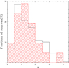 |
Fig. 1. Redshift distribution for full hard sample (solid histogram), and CT AGN with probabilities > 90% described in Sect. 4 (shaded histogram). |
We reduced all the Chandra survey data in a uniform manner as described in Laird et al. (2009) with the CIAO data analysis software version 4.8. We used the SPECEXTRACT script in the CIAO package to extract source spectra (with an extraction radius increasing as a function of the off-axis angle to enclose 90% of the point spread function at 1.5 keV), as well as response and auxiliary matrices, for each individual observation. The spectral data from each observation were then merged to create a single source spectrum, response, and auxiliary matrices for each source using the FTOOL tasks MATHPHA, ADDRMF, and ADDARF, respectively. Background spectra were extracted in five different source-free regions for each observation. Then, for each source, the closest background region among these five was selected and then merged for each source by taking each source detection (or non-detection) for each observation into account. Since sources near the edges of the field may not be present in all individual observations because of variations in the aim points and roll angles, the final exposure times range between 400 ks and 6.6 Ms. The net (background subtracted) counts distribution in the full (0.5−8 keV) band is presented in Fig. 2.
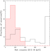 |
Fig. 2. Net (background subtracted) full (0.5−8 keV) band counts for full hard sample (solid histogram), and CT AGN with probabilities > 90% described in Sect. 4 (shaded histogram). The last bin in the solid histogram corresponds to the total percentage of sources with more than 800 counts. |
3. Automated spectral analysis
By comparing the different results obtained throughout the years for the same sources (Norman et al. 2002; Tozzi et al. 2006; Comastri et al. 2011; Georgantopoulos et al. 2013; Brightman et al. 2014; Buchner et al. 2014; Liu et al. 2017), it is clear that CT classification is model and data-quality dependent. Although the sample used in this work is rather small, our aim is to use it to develop an automated spectral selection method the least model-dependent as possible that may be applied to large samples of X-ray spectra spanning a wide range in data quality, such as the samples from surveys already carried out by Chandra and XMM-Newton, and also the ones expected to be carried out by the upcoming X-ray missions SRG/eROSITA1 and Athena2. The main characteristic of our method is that we do not classify sources as CT or not, but we derive the probability of a source being CT (Akylas et al. 2016). Therefore in this work, we consider that an AGN is a CT candidate if the resulting probability of the AGN being CT is larger than zero.
We used Xspec v12.9 (Arnaud 1996) to carry out the spectral analysis. We selected Cash statistics applied to spectra binned to 1 counts/bin, which allow us to obtain reliable spectral results even for low count data.
Given the data quality among our sample, we selected the following set of models, listed in increasing complexity order, to be applied to our data:
-
An absorbed power-law plus a Gaussian emission line: Xspec:zwabs*zpo+zgaus. The Gaussian component is intended to represent the Fe Kα emission line, the most often observed emission line in AGN X-ray spectra. In CT AGN, the equivalent width (EW) of this line is expected to be very high, sometimes over 1 keV.
-
A double power-law plus a Gaussian line: zwabs*zpo+zpo+zgaus. The unabsorbed power-law can represent either soft-scattering of the primary (hard) power-law emission, or transmitted emission in the case of a partial covering absorber.
-
A modified power-law by a toroidal-shaped absorber plus a soft-scattered component: torus+zpo, where torus correspond to the model described in Brightman & Nandra (2011). This model is a more appropriate model for our highly absorbed sources since it consistently takes into account photoelectric absorption, fluorescence line emission (Fe Kα), and Compton scattering. The parameters of this model are, besides the column density, photon index, and normalization, the torus opening angle and its inclination with respect to the observer. We fixed this angles to 60 and 80°, respectively (see the following discussion).
Out of the three spectral models described above, the last one is the more physically-motivated one. However, high data quality is needed to fit both the opening and inclination angles at the same time. Fixing the opening angle to 60° and the inclination angle to 80° is a good approximation in the case of modeling highly absorbed and CT AGN spectra, but it is not always a good choice for less absorbed sources. For moderately to low absorbed sources, the derived column densities depend more strongly on the inclination angle than for highly absorbed ones (Lanzuisi et al. 2018). Whereas simple models, like the first two, have been proven to be a good representation of the spectral shape up to column densities of 1023 cm−2 (Liu et al. 2017). It is important to remember that, up to this point, we are not trying to derive the best-fit model parameters but to characterize the spectral shape well enough to be able to pinpoint highly absorbed sources.
Therefore, we proceeded with the following two steps: we applied the first two models to all of our sample, and then we only applied the torus model to sources displaying high absorption features in their spectra. We looked for these features by using the spectral-fitting results of the first two models (see Sect. 3.1 and Corral et al. 2014).
3.1. Optimization of the automated spectral analysis
Instead of fitting a highly-absorbed-AGN oriented model (the torus model) to all of our sources, we made use of the automated selection technique for highly obscured AGN presented in Corral et al. (2014). This is a fast, less model-dependent, and reliable way to pinpoint heavily obscured sources without the need to apply complex models that could be biased toward certain kinds of AGN. This method uses very simple spectral models (an absorbed power-law: zwabs*zpo+zgaus; and a double power-law: zwabs*zpo+zpo+zgaus) to select sources as highly absorbed candidates by pinpointing signatures of obscuration.
To define a region in the best-fit spectral parameters space so that all CT sources would be selected, we refined the selection technique presented in Corral et al. (2014) by using simulations. We simulated each source and background in our sample five times by varying the column density from 1022 to 1025 cm−2, while also preserving their fluxes and redshifts. For column densities below 5 × 1023 cm−2 we used the Xspec model plcabs (Yaqoob 1997) to reproduce the absorbed power law, whereas for CT column densities, we used the mytorus self-consistent model (Murphy & Yaqoob 2009). In both cases, an additional soft-scattered power-law component was also included with a maximum scattered fraction of 10% with respect to the primary emission. We then applied our simple models to the simulated data. In order to down-select all the CT sources, the best-fit parameter for the considered models had to fulfill at least one of the following selection criteria: the measured column density is in the CT regime (> 1024 cm−2); the power-law photon index is flat (< 1.4), either in the hard 2−10 keV band or in the rest-frame hard band, and the column density value is lager than 5 × 1023 cm−2; the power-law photon index is flat (< 1.4), either in the hard 2−10 keV band or in the rest-frame hard band, and the Fe Kα emission line EW is larger than 500 eV; and for sources with the lowest number of counts in the 2−8 keV band, and thus a limiting reliability of the spectral fits, we only require that the power-law photon index is flat (< 1.4), either in the hard 2−10 keV band or in the rest-frame hard band.
By using these criteria, we ensure that all the CT AGN are selected, albeit including a significant percentage of low (≤6%; NH < 1023 cm−2) and highly, but not CT, absorbed sources (≤17%; 1023 cm−2 < NH < 1024 cm−2).
3.2. Data quality effects
We also used the simulations described in the previous section to quantify how the data quality could limit our results. We applied the torus model described in Sect. 3 to all of the simulated data, thus obtaining the values displayed in Fig. 3. There are two clear problematic regions in this plot labeled FP (false positives) and M (missing CT AGN).
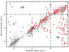 |
Fig. 3. Simulated column densities (Xspec: zwabs,plcabs,mytorus) versus best-fit (recovered) column densities (Brightman & Nandra 2011 torus model). Filled (red) circles correspond to highly absorbed candidates (see Sect. 3.1). FP: false positives. M: missing CT AGN. |
The most populated among the problematic regions in Fig. 3 is region M, which corresponds to simulated CT AGN that are not identified as such when fit by the torus model. All these simulations are associated with spectra with less than 100 counts in the hard (2−8 keV) band. Given the spectral counts distribution in our sample, this implies that we could miss up to 14% of CT candidates in the case of spectra with less than 100 counts, that is, we could miss six CT candidates of our actual sample due to low data quality alone.
The second problematic, but much less populated, region in Fig. 3 is the FP region, which corresponds to sources misidentified as CT candidates when fit by the torus model. These simulations also correspond to spectra with less than 100 counts in the hard band, and they could amount to up to 2% (only one source in the actual sample) of misclassified CT candidates.
By combining the results from Sect. 3.1 and the ones presented in this section, we can estimate the number of missing and/or misclassified CT candidates in the following analyses (see Sect. 5.2).
4. Bayesian CT probabilities
By applying the selection technique described in Sect. 3.1 to our actual sample, we ended up with 59 highly absorbed candidates. According to our simulations, most of these sources should be at least highly absorbed (NH > 1023 cm−2), and all of the CT AGN in our sample should be within these 59 candidates.
As mentioned at the end of Sect. 3, once we identified the sources most likely to be CT AGN within our sample, we applied a more appropriate model to them in order to obtain our final spectral results as follows: the torus model described in Brightman & Nandra (2011) and a second power law that accounts for soft scattered emission. From the spectral results of this model, we confirm that most (∼90%) of our candidates are in fact highly absorbed AGN.
Instead of basing a CT classification on the best-fit column density, we adopted the Bayesian approach described in Akylas et al. (2016). This approach is based in the derivation of the probability distributions for each variable spectral parameter by using Monte Carlo Markov chains (MCMC) and the Goodman-Weare algorithm. In this way, instead of classifying a source as CT or not, we assign a probability of the CT source by integrating the probability distribution of the column density above 1024 cm−2. In applying this method, we find that 36, out of the initial 59 sources, have a probability higher than zero of being CT (PCT > 0); 20 of them have probabilities > 90% (see Fig. 5 and Table 1). Taking the probabilities for all of the 36 candidates into account, the effective number of CT AGN in our sample is 27.
Spectral fits results for candidate CT AGN.
It is important to remember that our intention is not to classify sources as CT AGN nor to derive the actual column densities of our sources, but to derive the probability of being CT (PCT). Therefore, the comparison presented in the last column of Table 1 must only be considered qualitatively and not as a direct comparison (see Sect. 5.1). We tested that by applying different models such as plcabs, mytorus, and/or by adding reflection (Xspec: pexmon), whereas changing the resulting values for the best-fit column densities did not significantly affect the resulting integrated probabilities over 1024 cm−2.
5. Discussion
5.1. Comparison with previous results
Brightman et al. (2014), Buchner et al. (2014), and Liu et al. (2017) performed systematic studies of CT AGN within the CDF-S by using Chandra data, finding nine, eight, and ten candidate CT AGN, respectively. However, their CT classifications are not consistent with each other in many cases, being that 15 AGN is the combined number of candidates from those works. Brightman et al. (2014), Buchner et al. (2014) used 4 Ms CDF-S spectral data but not exactly the same sources, whereas Liu et al. (2017) used 7 Ms data but only presented the spectral analysis for the brighter sources in that catalog.
In this work, we derived CT probabilities > 90% for only 10 out of the 15 previously reported CT AGN included in Brightman et al. (2014), Buchner et al. (2014), and Liu et al. (2017) (see Table 1). For the remaining 5 AGN previously classified as CT, we find them only moderately to highly absorbed, except for source 180 which we find to be near-CT (probability ∼89%). More importantly, we find nine additional CT AGN with probabilities > 90% that were not classified as such in any of those works. Three of them were previously classified as near-CT. Another one, source 327 (Luo et al. 2008 ID), was not included in any of the samples used in Brightman et al. (2014), Buchner et al. (2014), and Liu et al. (2017). For the remaining five, either the column density, the power-law photon index, or both, were fixed during the previous spectral fits, which could explain the different results. In the case of sources 138, 266, and 312, the differences could be also due to the improved spectral quality in the 7 Ms data, since these sources are not included in the Liu et al. (2017) sample. New CT candidates are mainly due to lower number of counts in Brightman et al. (2014), Buchner et al. (2014), which used 4 Ms data, or because the sources are not included in either of the Brightman et al. (2014), Buchner et al. (2014), and Liu et al. (2017) samples.
5.2. Comparison with X-ray background synthesis models
We compared our CT number count distribution with the most recent cosmic X-ray background (CXB) synthesis models of Akylas et al. (2012) and Ueda et al. (2014). In our case, we weighted each of our candidate CT by the probability of them being CT (see Akylas et al. 2016), so that the number integral number count, N(> S), of sources per unit sky area with flux higher than S is defined as follows:
where we summed all the sources with fluxes Si > Sj at each bin, and Ωi represents the sky coverage as a function of flux from the 2 Ms survey (Luo et al. 2008).
Instead of computing the errors in each bin, we estimated a confidence interval by performing simulations. According to the results from Sect. 3.2, we could be missing up to 6 CT candidates, and one of our candidates could have been wrongly selected. We also know that these seven sources have to fulfill the selection criteria described in Sect. 3.1, that is, they must be among the 59 highly absorbed candidates with derived PCT = 0. Besides, their spectra must have less than 100 counts in the hard band. Taking all of this into account, we simulated 10 000 realizations in which we added up to six sources (simulated following the fluxes of the highly absorbed candidates with less than 100 counts, and with random PCT), and randomly removed one of the actual CT candidates. We considered our confidence interval to be the region that encompasses 99.7% of our simulated number count distributions (gray area in Fig. 4).
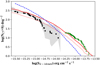 |
Fig. 4. Number count distribution of CT AGN (circles) in CDF-S (this work) and for COSMOS-Legacy data in Lanzuisi et al. (2018) (crosses). Solid and dotted lines correspond to the model predictions presented in Akylas et al. (2012) for a CT fraction of 15% plus 5% reflection, and for a CT fraction of 25%, respectively. The dashed line corresponds to the model in Ueda et al. (2014). |
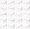 |
Fig. 5. X-ray unfolded spectra for candidate CT AGN with probabilities > 90%. |
Our results are plotted in Fig. 4. As a comparison, we plotted the models of Akylas et al. (2012) for a 15% CT fraction and 5% of the reflected emission, for a 25% CT fraction, and the model of Ueda et al. (2014), which assumes a large (∼50%) percentage of CT AGN and only a moderate amount of reflection. One of the main differences between both models is that the Ueda et al. (2014) model has an extra free parameter allowing for differential evolution of the CT AGN population relative to the population of unobscured and mildly obscured AGN. We also plotted the results from Lanzuisi et al. (2018), which also use Chandra data but from the 3 Ms COSMOS-Legacy survey (Civano et al. 2016). In that work, they also derived the probability distribution for the column densities and use them in a similar way as we did in this work. Our results look more consistent with the model proposed in Akylas et al. (2012) for a 25% percentage of CT AGN, a smaller value than the one presented in Lanzuisi et al. (2018). They report a number density of CT AGN which increases from 30 to 55% with redshift. Because of the relative small size of our sample, we cannot test this evolution with redshift in our case. A very recent work that also makes use of the CDF-S 7 Ms data, although a different spectral analysis was carried out in that case, reports a moderate fraction of CT when computing their number counts (Li et al. 2019), which is consistent with our results. Although smaller fractions and/or CXB models with higher amounts of reflection are also consistent within errors, local studies point to small amounts of reflection (Georgantopoulos & Akylas 2019).
6. Conclusions
We used the deepest X-ray observation to date, the 7 Ms Chandra observation of the CDF-S, to search for CT AGN in the hard (2−8 keV) selected sample presented in Luo et al. (2008), which is based on a shallower 2 Ms observation. In this way, we were able to improve previous spectral analyzes and to better constrain the intrinsic column densities of the sources in our sample. Moreover, by making use of simulations, we estimate that among X-ray spectra with less than 100 counts in the hard band (2−8 keV), X-ray analyses could be missing ∼14% of the CT AGN just because of the data quality.
To optimize the automated spectral analysis and to quantify data-quality effects, we applied an automated selection technique to select highly absorbed candidates, and then we applied a Bayesian method to compute the probability of a source being CT. We find 36 CT candidates with probabilities larger than zero, and 20 with probabilities > 90%. Nine of them are classified as CT for the first time thanks mostly to the deeper 7 Ms data. Our results are in good agreement with previous results, although we do not confirm the previous CT classification of five sources. We find that one source is near-CT, and that the other four look to be only moderately absorbed.
We used the computed probabilities to derive the number count distribution of CT AGN in the CDF-S. By comparing our findings with the CXB synthesis models in Ueda et al. (2014) and Akylas et al. (2012), our results favor the one presented in Akylas et al. (2012) assuming a percentage of 25% CT AGN.
Acknowledgments
We thank the referee for his/her helpful comments and suggestions. The Chandra data were taken from the Chandra Data Archive at the Chandra X-ray Center. AC acknowledges funding from ESA under the PRODEX project and financial support through grant AYA2015-64346-C2-1-P (MINECO/FEDER). AC is supported by a “Juan de la Cierva Incorporación” postdoctoral contract from Ministerio de Ciencia, Innovación y Universidades (Spain).
References
- Akylas, A., Georgakakis, A., Georgantopoulos, I., Brightman, M., & Nandra, K. 2012, A&A, 546, A98 [NASA ADS] [CrossRef] [EDP Sciences] [Google Scholar]
- Akylas, A., Georgantopoulos, I., Ranalli, P., et al. 2016, A&A, 594, A73 [NASA ADS] [CrossRef] [EDP Sciences] [Google Scholar]
- Alexander, D. M., Stern, D., Del Moro, A., et al. 2013, ApJ, 773, 125 [NASA ADS] [CrossRef] [Google Scholar]
- Arnaud, K. A. 1996, in Astronomical Data Analysis Software and Systems V, eds. G. H. Jacoby, & J. Barnes, ASP Conf. Ser., 101, 17 [NASA ADS] [Google Scholar]
- Brandt, W. N., & Alexander, D. M. 2015, A&ARv, 23, 1 [Google Scholar]
- Brightman, M., & Nandra, K. 2011, MNRAS, 413, 1206 [CrossRef] [Google Scholar]
- Brightman, M., Nandra, K., Salvato, M., et al. 2014, MNRAS, 443, 1999 [NASA ADS] [CrossRef] [Google Scholar]
- Buchner, J., Georgakakis, A., Nandra, K., et al. 2014, A&A, 564, A125 [NASA ADS] [CrossRef] [EDP Sciences] [Google Scholar]
- Civano, F., Marchesi, S., Comastri, A., et al. 2016, ApJ, 819, 62 [NASA ADS] [CrossRef] [Google Scholar]
- Comastri, A., Ranalli, P., Iwasawa, K., et al. 2011, A&A, 526, L9 [NASA ADS] [CrossRef] [EDP Sciences] [Google Scholar]
- Corral, A., Georgantopoulos, I., Watson, M. G., et al. 2014, A&A, 569, A71 [NASA ADS] [CrossRef] [EDP Sciences] [Google Scholar]
- Croom, S. M., Richards, G. T., Shanks, T., et al. 2009, MNRAS, 399, 1755 [NASA ADS] [CrossRef] [Google Scholar]
- Georgantopoulos, I., & Akylas, A. 2019, A&A, 621, A28 [NASA ADS] [CrossRef] [EDP Sciences] [Google Scholar]
- Georgantopoulos, I., Comastri, A., Vignali, C., et al. 2013, A&A, 555, A43 [NASA ADS] [CrossRef] [EDP Sciences] [Google Scholar]
- Harrison, F. A., Aird, J., Civano, F., et al. 2016, ApJ, 831, 185 [NASA ADS] [CrossRef] [Google Scholar]
- Hickox, R. C., & Alexander, D. M. 2018, ARA&A, 56, 625 [Google Scholar]
- Hsu, L.-T., Salvato, M., Nandra, K., et al. 2014, ApJ, 796, 60 [NASA ADS] [CrossRef] [Google Scholar]
- Laird, E. S., Nandra, K., Georgakakis, A., et al. 2009, ApJS, 180, 102 [NASA ADS] [CrossRef] [Google Scholar]
- Lanzuisi, G., Civano, F., Marchesi, S., et al. 2018, MNRAS, 480, 2578 [NASA ADS] [CrossRef] [Google Scholar]
- Li, J., Xue, Y., Sun, M., et al. 2019, ApJ, 877, 5 [NASA ADS] [CrossRef] [Google Scholar]
- Liu, T., Tozzi, P., Wang, J.-X., et al. 2017, ApJS, 232, 8 [NASA ADS] [CrossRef] [Google Scholar]
- Luo, B., Bauer, F. E., Brandt, W. N., et al. 2008, ApJS, 179, 19 [NASA ADS] [CrossRef] [Google Scholar]
- Luo, B., Brandt, W. N., Xue, Y. Q., et al. 2010, ApJS, 187, 560 [NASA ADS] [CrossRef] [Google Scholar]
- Luo, B., Brandt, W. N., Xue, Y. Q., et al. 2017, ApJS, 228, 2 [Google Scholar]
- Murphy, K. D., & Yaqoob, T. 2009, MNRAS, 397, 1549 [NASA ADS] [CrossRef] [Google Scholar]
- Norman, C., Hasinger, G., Giacconi, R., et al. 2002, ApJ, 571, 218 [NASA ADS] [CrossRef] [Google Scholar]
- Ricci, C., Ueda, Y., Koss, M. J., et al. 2015, ApJ, 815, L13 [NASA ADS] [CrossRef] [Google Scholar]
- Tozzi, P., Gilli, R., Mainieri, V., et al. 2006, A&A, 451, 457 [NASA ADS] [CrossRef] [EDP Sciences] [Google Scholar]
- Ueda, Y., Akiyama, M., Hasinger, G., Miyaji, T., & Watson, M. G. 2014, ApJ, 786, 104 [NASA ADS] [CrossRef] [Google Scholar]
- Xue, Y. Q., Luo, B., Brandt, W. N., et al. 2011, ApJS, 195, 10 [NASA ADS] [CrossRef] [Google Scholar]
- Yaqoob, T. 1997, ApJ, 479, 184 [NASA ADS] [CrossRef] [Google Scholar]
All Tables
All Figures
|
Fig. 1. Redshift distribution for full hard sample (solid histogram), and CT AGN with probabilities > 90% described in Sect. 4 (shaded histogram). |
| In the text | |
|
Fig. 2. Net (background subtracted) full (0.5−8 keV) band counts for full hard sample (solid histogram), and CT AGN with probabilities > 90% described in Sect. 4 (shaded histogram). The last bin in the solid histogram corresponds to the total percentage of sources with more than 800 counts. |
| In the text | |
|
Fig. 3. Simulated column densities (Xspec: zwabs,plcabs,mytorus) versus best-fit (recovered) column densities (Brightman & Nandra 2011 torus model). Filled (red) circles correspond to highly absorbed candidates (see Sect. 3.1). FP: false positives. M: missing CT AGN. |
| In the text | |
|
Fig. 4. Number count distribution of CT AGN (circles) in CDF-S (this work) and for COSMOS-Legacy data in Lanzuisi et al. (2018) (crosses). Solid and dotted lines correspond to the model predictions presented in Akylas et al. (2012) for a CT fraction of 15% plus 5% reflection, and for a CT fraction of 25%, respectively. The dashed line corresponds to the model in Ueda et al. (2014). |
| In the text | |
|
Fig. 5. X-ray unfolded spectra for candidate CT AGN with probabilities > 90%. |
| In the text | |
Current usage metrics show cumulative count of Article Views (full-text article views including HTML views, PDF and ePub downloads, according to the available data) and Abstracts Views on Vision4Press platform.
Data correspond to usage on the plateform after 2015. The current usage metrics is available 48-96 hours after online publication and is updated daily on week days.
Initial download of the metrics may take a while.