| Issue |
A&A
Volume 618, October 2018
|
|
|---|---|---|
| Article Number | A76 | |
| Number of page(s) | 4 | |
| Section | Stellar atmospheres | |
| DOI | https://doi.org/10.1051/0004-6361/201833271 | |
| Published online | 15 October 2018 | |
CXOU J160103.1–513353: another central compact object with a carbon atmosphere?
1
Institut für Astronomie und Astrophysik, Sand 1, 72076 Tübingen, Germany
e-mail: This email address is being protected from spambots. You need JavaScript enabled to view it.
2
Space Research Institute of the Russian Academy of Sciences, Profsoyuznaya Str. 84/32, Moscow, 117997 Russia
3
Kazan (Volga region) Federal University, Kremlevskaja str., 18, Kazan, 420008, Russia
Received:
20
April
2018
Accepted:
14
June
2018
Abstract
We report on the analysis of XMM-Newton observations of the central compact object CXOU J160103.1–513353 located in the center of the non-thermally emitting supernova remnant (SNR) G330.2+1.0. The X-ray spectrum of the source is well described with either single-component carbon or two-component hydrogen atmosphere models. In the latter case, the observed spectrum is dominated by the emission from a hot component with a temperature ∼3.9 MK, corresponding to the emission from a hotspot occupying ∼1% of the stellar surface (assuming a neutron star with mass M = 1.5 M⊙, radius of 12 km, and distance of ∼5 kpc as determined for the SNR). The statistics of the spectra and obtained upper limits on the pulsation amplitude expected for a rotating neutron star with hot spots do not allow us to unambiguously distinguish between these two scenarios. We discuss, however, that while the non-detection of the pulsations can be explained by the unfortunate orientation in CXOU J160103.1–513353, this is not the case when the entire sample of similar objects is considered. We therefore conclude that the carbon atmosphere scenario is more plausible.
Key words: stars: atmospheres / stars: neutron / X-rays: stars
© ESO 2018
1. Introduction
The central compact object (CCO) CXOU J160103.1–513353 was discovered with Chandra at the center of the supernova remnant (SNR) G330.2+1 by Park et al. (2006). The origin of the source was established based on the absence of counterparts in other wavebands and on the observed blackbody like spectrum with kT ∼ 0.5 keV typical for other CCOs. Park et al. (2006) also claimed the tentative detection of pulsations from the source with a period of ∼7.5 s and an amplitude of ∼30 %, which would clearly establish the object as a neutron star. However, follow-up observations with XMM-Newton refuted this detection (Park et al. 2009). Poor counting statistics only allowed to place an upper limit on the pulsed fraction PF = (Fmax − Fmin)/(Fmax + Fmin) of ∼40 %. This is significantly higher than that observed in other CCOs, which means that observations were likely not sensitive enough to detect pulsations from the source.
The source, however, is expected to pulsate. While the observed X-ray spectrum could be described as a uniformly emitting neutron star hydrogen atmosphere, this results in unreasonably large distances ≥24 kpc for standard neutron star parameters (Park et al. 2009). The actual distance to the SNR was estimated by McClure-Griffiths et al. (2001) at ∼5 kpc based on the observed H I absorption in radio, which implies a significantly smaller emission region size. Park et al. (2009) therefore concluded that the observed emission predominantly arises from hotspots with radii of 0.3–2 km, while the remaining surface is significantly cooler and does not contribute much to the observed flux. This scenario was first proposed by Pavlov et al. (2000) for the CCO in Cas A, and it implies that the source must pulsate, which has not been observed so far.
In addition to the limited sensitivity of the observations, the non-detection of the pulsations might be explained by geometrical considerations, that is, alignment of the spin axis of the neutron star with the magnetic field or with the line of sight (Suleimanov et al. 2017), especially given the existing modest constraints on the observed pulsed fraction. Alternatively, the lack of pulsations can be explained if the observed X-ray emission does arise from the entire surface of the neutron star whose atmosphere is composed of heavier elements such as carbon (Ho & Heinke 2009, 2013, 2015, 2016). This is an intriguing option as pure hydrogen atmospheres are commonly assumed to interpret thermally emitting neutron star observations (Pavlov et al. 2004). Such observations are considered one of the prime probes for the equation of state of matter under supra-nuclear densities, and thus are of fundamental importance (Lattimer & Prakash 2007, 2016).
The possibility that the atmosphere consists of heavier elements despite presumably fast stratification complicates the interpretation of the observations, so that additional observational information such as cooling of the neutron star must be considered in this case (Ofengeim et al. 2015). On the other hand, detection and observed amplitude of the pulsations must also be taken into consideration. For instance, Bogdanov (2014) demonstrated that the spectrum of another thermally emitting neutron star PSR J1852+0040 in SNR Kes 79 can be well described with a single-temperature carbon atmosphere. However, strong pulsations are observed in this case, which suggest that caution must be taken when making any conclusions based on the observed spectrum alone.
We here discuss CXOU J160103.1–513353 in this context. Using the new 150 ks XMM-Newton observation of the source, we obtain improved X-ray spectra and upper limits on the fraction of pulsed emission. We conclude that observations are fully consistent with the carbon atmosphere scenario. On the other hand, the available data do not allow us to univocally exclude the two-temperature hydrogen atmosphere model based on non-detection of the pulsations, so that additional observations might be required. Nevertheless, a rather particular geometry is required to explain the absence of pulsations in this and several other non-pulsating CCOs, which suggests that the a single carbon atmosphere model might still be preferred.
2. Data analysis and results
The source has been observed with Chandra (Park et al. 2006), ASCA (Torii et al. 2006), and several times with XMM-Newton. Here we use data from the two longest XMM observations: obsid. 0500300101 (68 ks) and 0742050101 (140 ks). The first observation is significantly affected by in-orbit background, and has previously been used by Park et al. (2009) to characterize the spectrum of the CCO, while the second observation has only been used so far to study the extended emission from the SNR by Williams et al. (2018), who confirmed the nonthermal origin of the extended emission and strong absorption in the direction of the source with an equivalent column of ∼2–3 × 1022 cm−2.
The data reduction was carried out according to the XMM user guide using the XMM SAS version 16.1.0 and a current set of calibration files. Both pointings were contaminated by soft proton background to some extent, so that after the standard screening, the effective exposures were reduced to ∼35 ks and 93/110 ks (PN/MOS) for the first and second observations, respectively. We only used EPIC MOS data for the first observation since the PN was operated in small-window mode, with some extended emission falling within the storage area and thus increasing the background. Together with uncertainties in calibration in small-window mode, this made this pointing not very useful for spectral analysis, and a timing analysis has previously been published by Park et al. (2006).
The spectrum of the source and events for timing analysis were extracted from a circle with a radius of 28″ centered on the coordinates reported by Park et al. (2006). The extraction radius was selected to optimize the signal-to-noise ratio with the help of the eregionanalyse task. The background was extracted from two circles with the same radius adjacent to the source with the same RAWY coordinate to ensure that similar low-energy noise was subtracted for EPIC PN1. Two background regions were selected to account for possible variations in brightness of the extended emission. We verified that results were not significantly affected when the background was extracted from an annulus around the source (which is, however, not recommended, as detailed in the same calibration note). The same source background regions were also used for the MOS cameras.
2.1. Spectral analysis
Source spectra were extracted for two observations and three cameras and were simultaneously fit together after binning to contain at least 25 counts/bin. As discussed by Park et al. (2006, 2009), a single blackbody or hydrogen atmosphere model results in an unrealistically large distance to the source. Therefore, we only considered the two-component, non-magnetic hydrogen and carbon atmosphere models (Suleimanov et al. 2014, 2017). To fit the spectra, we used Xspec version 12.9.1p, where both models are implemented (hatm and carbatm, respectively). Additionally, we included the TBabs absorption component and cross-normalization constants to account for interstellar absorption (Wilms et al. 2000) and effective area discrepancy between individual instruments. In both cases we assumed M = 1.5 M⊙ and R = 12 km for the neutron star, and a distance to the source of 4.9 kpc (McClure-Griffiths et al. 2001).
For the two-component fit the normalizations of the components were linked to each other through an additional constant 0 ≤ δ ≤ 1 defining the fraction of the surface area occupied by the hotspots (Suleimanov et al. 2017). In particular, we assumed that the model consists of two atmosphere model spectra of different temperatures with a free ratio of their emitting areas: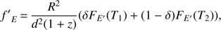
where the emitted E′ and the observed energies E of the photons are connected by the relation E′ = E(1 + z), where z = (1 − Rs/R)−1/2 − 1 and Rs = 2GM/c2 are the gravitational redshift and Schwarzschild radius, and d is the assumed distance to the source.
The best-fit results and a representative spectrum are presented in Table 1 and Fig. 1. Both models provide an adequate description of the data, and neither is statistically preferred.
It is interesting to note that both models require a significantly higher absorption column than that derived by Williams et al. (2018) for extended SNR emission (NH ≤ 3.13 × 10²² atoms cm−2). This mismatch might point to problems with the modeling of the extended emission spectrum or to an overestimation of the soft X-ray flux of the neutron star by atmosphere models, or it might indicate additional absorption specific to neutron star. We note that CXOU J160103.1–513353 is not the only object where the CCO emission appears to be more absorbed than the extended emission of the remnant. A comparison of the absorption columns reported by Klochkov et al. (2015) for CCO in SNR G353.6-0.7 and by Doroshenko et al. (2017) for the extended emission around the neutron star also reveals an enhanced absorption for the compact object.
The large difference in temperature of the two components and the high absorption column in the two-component fit also implies that most of the flux from the cold surface of the neutron star is not observed. The emission from the hotspots therefore dominates the observed flux, which contributes ∼82%. This is in line with the analysis results of the first observation by Park et al. (2009), who found that the soft component is not statistically required by the fit.
2.2. Timing analysis
We also exploited the additional exposure provided by the new data to improve the ∼40% upper limit on the pulsed fraction obtained by Park et al. (2009) based on the first XMM observation. Other CCOs have short periods, therefore the important constraint here was provided by EPIC PN data, which offered 5.7 ms time resolution in small-window mode. Unfortunately, the obtained limit is not particularly constraining because of the high background level (∼30%), and we were unable to significantly improve it. On the other hand, EPIC MOS operated in full-frame mode and thus is only sensitive for periods above ∼5.2 s, which is not enough by far to probe the ∼100 ms periods typical for CCOs (Gotthelf et al. 2013).
The time resolution of EPIC PN in full-frame mode used for the second observation is ∼73 ms, which is not sufficient either to probe timescales quite as short as this. However, pulsations with periods longer ∼147 ms can be probed, and at least one CCO has a period in this range. The observation is also longer by a factor of three than the first one and has a lower level of in-orbit background, which significantly increases the sensitivity to the pulsations in the accessible range of periods and thus allows us to improve on the upper limits obtained by Park et al. (2009). The upper limits for the MOS data can likewise clearly be improved, so that we considered a period range of 147 ms to 100 s for EPIC PN data and 5.2–100 s for the combined data set including data from both cameras.
To search for the pulsations and estimate upper limits on the pulsed fraction, we used the same methods as Doroshenko et al. (2015). First, we optimized the energy range and extraction radius for the source in order to obtain the highest signal-to-noise ratio. The energy range was chosen to minimize contribution of the background (mostly extended emission from the SNR). Then the optimal extraction radius of 28″ was estimated with the eregionanalyse task for the obtained energy range of 1.7–4.2 keV. Coincidentally, this energy range also mostly excludes photons from the cool component in the two-component atmosphere model, which means that the intrinsic pulsations must also be the strongest. After the extraction, the photon arrival times were corrected for using the barycen task, and a search for pulsations was carried out using the H-test of de Jager et al. (1989). Similarly to Park et al. (2006), we oversampled the search frequency grid by factor of ten to ensure that no peaks were missed. In line with the previous findings, no significant pulsed signal was found.
To estimate the upper limit on the pulsed fraction, we followed the approach by Brazier (1994), Doroshenko et al. (2015) and repeated the procedure separately for the combined MOS/PN and PN data. The strictest upper limits were obtained by combining both observations (assuming that the period of the source did not change), although we also carried out a timing analysis for individual observations. For periods in the range of 5.2–100 s, 4520 photons (including ∼11% background) were detected from all detectors combined in two observations (also including PN data from the first observation). For the maximum test statistics of 15.4, this implies a 3σ upper limit of ∼16%. The best limit for the PN data alone is again obtained when both observations are combined (period search restricted to 147 ms 100 s to match the resolution of the full frame data), which yields 2330 photons including 12% background, a peak statistics value of 17.4, and an upper limit on the pulsed fraction of 21% in a period range of 147 ms to 100 s. The upper limit for shorter periods using the PN data from the first observation was found to be consistent with the limit reported by Park et al. (2006), that is, ∼45%.
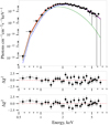 |
Fig. 1. Best-fit unfolded spectrum (top panel) and residuals for the two-component hydrogen atmosphere (middle panel) and carbon models (bottom panel). Only the EPIC PN spectrum from observation 0742050101 is shown for clarity. The contribution of the cold and hot components to the two-component fit is shown with thin lines. The total model flux is indistinguishable for the two models and is shown with the thick red line. |
Best-fit parameters for the two-component hydrogen and carbon atmosphere models assuming a distance fixed to 4.9 kpc.
3. Discussion and conclusions
A rotating neutron star will be observed to pulsate only when the hotspots are misaligned with the rotation axis and the rotation axis itself does not point directly to the observer. The expected pulsed fraction depends thus on the geometrical configuration of the hotspots and on the orientation of the pulsar with respect to the observer. This problem was discussed by Elshamouty et al. (2016) for quiescent low-mass X-ray binaries and by Suleimanov et al. (2017) for other CCOs. In particular, Suleimanov et al. (2017) calculated the probability that pulsation in this source escaped detection given the existing limits on the pulsed fraction and hotspot size, and assuming a random location of the hotspots and orientation of the neutron star with respect to the observer. Suleimanov et al. (2017) considered the angular distribution of the emission emerging from the atmosphere and its propagation to the observer in the strong gravitational field of the neutron star. These authors concluded that there is only an ∼8% chance probability that pulsations are not observed.
Here we repeated the analysis presented by Suleimanov et al. (2017) for CXOU J160103.1–513353. We used the limits on pulsed fraction and best-fit spectral parameters for the two-component hydrogen atmosphere obtained in the previous section as input. The results are presented in Fig. 2, which is similar to Fig. 14 of Suleimanov et al. (2017). Unfortunately, the sensitivity of the observations does not allow us to place strong constraints on the orientation of the neutron star, so that the probabilities that the pulsations are not detected as a result of unfavorable geometry are quite high: ∼18.5% for PF ≤ 16% and ∼30% for PF ≤ 21%. Significantly longer exposures would be required to obtain stronger constraints. We therefore conclude that the available data do not allow us to rule out the two-component scenario based on the non-detection of the pulsations.
On the other hand, it is important to mention that CXOU J160103.1–513353 is not the only object for which the two-component scenario has been invoked and yet no pulsations have been detected. As discussed by Suleimanov et al. (2017), in each individual case, the probability of a non-detection of the pulsations as a result of unfavorable geometry is not negligible, but it is quite unlikely that the geometry is unfavorable for all sources. We currently know of four neutron stars that are presumably covered by carbon envelopes: CCOs in SNRs Cas A, HESS J1731−347, G15.9+02, and G330.2+1. None of them exhibits pulsation, and the joint probability is sufficiently low for the geometry to be unfavorable. Considering the CCOs in HESS J1731+347 and Cas A, Suleimanov et al. (2017) estimated a joint probability that both these CCOs have unfavorable viewing angles toward us at ∼1%. This probability becomes even lower, about 0.3%, if CXOU J160103.1–513353 is considered. While a non-detection of the pulsations in this group of CCOs could also be explained by some systematic process aligning the field of the neutron star with the rotation axis, it is unclear why the same process would not be effective for the pulsating CCO population. We therefore have to conclude that a separate population of CCOs might exist whose atmospheres predominantly consist of heavier elements.
If this is indeed the case, it is important to understand the mechanisms responsible for the enrichment of the atmosphere with heavier elements. Chang et al. (2010) suggested that in absence of accretion, diffusive nuclear burning (DNB) of hydrogen and helium might be such a mechanism. This scenario requires, however, that the accretion is inhibited almost completely. Chang et al. (2010) argued that a pulsar wind might be responsible for inhibiting the accretion, but did not discuss the potential effectiveness of this mechanism. On the other hand, Doroshenko et al. (2016) suggested that carbon in the atmosphere of the neutron star might be explained by the accretion of material that is enriched with heavier elements during the supernova explosion. The velocity of the expanding ejecta (∼10 000 km s−1) , which almost freely expands for about one hundred years (Branch & Wheeler 2017), is significantly higher than the typically observed kick velocities of neutron stars (∼300 km s−1). The compact object is therefore not expected to leave the metal-rich ejecta for several thousand years.
In the case of HESS J1731-347 discussed by Doroshenko et al. (2016), this suggestion is directly supported by the massive dust shell that encloses the CCO. The dust is likely also responsible for the enhanced absorption of the neutron star X-ray emission in this source we described above. While there is no evidence for dust in G330.2+1.0 we discussed here, the absorption column is similarly enhanced, which might point to additional material around the neutron star in this case as well. Alp et al. (2018) also recently discussed such a scenario in the context of X-ray absorption in young core-collapse SNRs, concluding that this might be the reason for the non-detection of a CCO in SN 1987A.
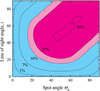 |
Fig. 2. Contours of constant PF in the θB − i plane. The permitted region with PF ≤ 16–21% (depending on the considered period range) is shown in blue. |
Acknowledgments
VD and AS thank the Deutsches Zentrum for Luft- und Raumfahrt (DLR) and Deutsche Forschungsgemeinschaft (DFG) for financial support. VS was supported by the German Research Foundation (DFG) grant WE 1312/48-1, and he also acknowledges support by the Russian Science Foundation through grant 14-12-01287.
References
- Alp, D., Larsson, J., Fransson, C., et al. 2018, ApJ, 864, 175 [NASA ADS] [CrossRef] [Google Scholar]
- Bogdanov, S. 2014, ApJ, 790, 94 [NASA ADS] [CrossRef] [Google Scholar]
- Branch, D., & Wheeler, J. C. 2017, Supernova Explosions (Berlin: Springer-Verlag GmbH) [CrossRef] [Google Scholar]
- Brazier, K. T. S. 1994, MNRAS, 268, 709 [NASA ADS] [Google Scholar]
- Chang, P., Bildsten, L., & Arras, P. 2010, ApJ, 723, 719 [NASA ADS] [CrossRef] [Google Scholar]
- de Jager, O. C., Raubenheimer, B. C., & Swanepoel, J. W. H. 1989, A&A, 221, 180 [NASA ADS] [Google Scholar]
- Doroshenko, V., Santangelo, A., & Ducci, L. 2015, A&A, 579, A22 [NASA ADS] [CrossRef] [EDP Sciences] [Google Scholar]
- Doroshenko, V., Pühlhofer, G., Kavanagh, P., et al. 2016, MNRAS, 458, 2565 [NASA ADS] [CrossRef] [Google Scholar]
- Doroshenko, V., Pühlhofer, G., Bamba, A., et al. 2017, A&A, 608, A23 [NASA ADS] [CrossRef] [EDP Sciences] [Google Scholar]
- Elshamouty, K. G., Heinke, C. O., Morsink, S. M., Bogdanov, S., & Stevens, A. L. 2016, ApJ, 826, 162 [NASA ADS] [CrossRef] [Google Scholar]
- Gotthelf, E. V., Halpern, J. P., & Alford, J. 2013, ApJ, 765, 58 [NASA ADS] [CrossRef] [Google Scholar]
- Ho, W. C. G., & Heinke, C. O. 2009, Nature, 462, 71 [NASA ADS] [CrossRef] [PubMed] [Google Scholar]
- Klochkov, D., Pühlhofer, G., Suleimanov, V., et al. 2013, A&A, 556, A41 [NASA ADS] [CrossRef] [EDP Sciences] [Google Scholar]
- Klochkov, D., Suleimanov, V., Pühlhofer, G., et al. 2015, A&A, 573, A53 [NASA ADS] [CrossRef] [EDP Sciences] [Google Scholar]
- Klochkov, D., Suleimanov, V., Sasaki, M., & Santangelo, A. 2016, A&A, 592, L12 [NASA ADS] [CrossRef] [EDP Sciences] [Google Scholar]
- Lattimer, J. M., & Prakash, M. 2007, Phys. Rep., 442, 109 [NASA ADS] [CrossRef] [Google Scholar]
- Lattimer, J. M., & Prakash, M. 2016, Phys. Rep., 621, 127 [NASA ADS] [CrossRef] [Google Scholar]
- McClure-Griffiths, N. M., Green, A. J., Dickey, J. M., et al. 2001, ApJ, 551, 394 [NASA ADS] [CrossRef] [Google Scholar]
- Ofengeim, D. D., Kaminker, A. D., Klochkov, D., Suleimanov, V., & Yakovlev, D. G. 2015, MNRAS, 454, 2668 [NASA ADS] [CrossRef] [Google Scholar]
- Park, S., Mori, K., Kargaltsev, O., et al. 2006, ApJ, 653, L37 [NASA ADS] [CrossRef] [Google Scholar]
- Park, S., Kargaltsev, O., Pavlov, G. G., et al. 2009, ApJ, 695, 431 [NASA ADS] [CrossRef] [Google Scholar]
- Pavlov, G. G., Zavlin, V. E., Aschenbach, B., Trümper, J., & Sanwal, D. 2000, ApJ, 531, L53 [NASA ADS] [CrossRef] [Google Scholar]
- Pavlov, G. G., Sanwal, D., & Teter, M. A. 2004, in Young Neutron Stars and Their Environments, eds. F. Camilo, & B. M. Gaensler, IAU Symp., 218, 239 [NASA ADS] [Google Scholar]
- Suleimanov, V. F., Klochkov, D., Pavlov, G. G., & Werner, K. 2014, ApJs, 210, 13 [NASA ADS] [CrossRef] [Google Scholar]
- Suleimanov, V. F., Klochkov, D., Poutanen, J., & Werner, K. 2017, A&A, 600, A43 [NASA ADS] [CrossRef] [EDP Sciences] [Google Scholar]
- Torii, K., Uchida, H., Hasuike, K., et al. 2006, PASJ, 58, L11 [NASA ADS] [CrossRef] [Google Scholar]
- Williams, B. J., Hewitt, J. W., Petre, R., & Temim, T. 2018, ApJ, 855, 118 [NASA ADS] [CrossRef] [Google Scholar]
- Wilms, J., Allen, A., & McCray, R. 2000, ApJ, 542, 914 [NASA ADS] [CrossRef] [Google Scholar]
All Tables
Best-fit parameters for the two-component hydrogen and carbon atmosphere models assuming a distance fixed to 4.9 kpc.
All Figures
|
Fig. 1. Best-fit unfolded spectrum (top panel) and residuals for the two-component hydrogen atmosphere (middle panel) and carbon models (bottom panel). Only the EPIC PN spectrum from observation 0742050101 is shown for clarity. The contribution of the cold and hot components to the two-component fit is shown with thin lines. The total model flux is indistinguishable for the two models and is shown with the thick red line. |
| In the text | |
|
Fig. 2. Contours of constant PF in the θB − i plane. The permitted region with PF ≤ 16–21% (depending on the considered period range) is shown in blue. |
| In the text | |
Current usage metrics show cumulative count of Article Views (full-text article views including HTML views, PDF and ePub downloads, according to the available data) and Abstracts Views on Vision4Press platform.
Data correspond to usage on the plateform after 2015. The current usage metrics is available 48-96 hours after online publication and is updated daily on week days.
Initial download of the metrics may take a while.