| Issue |
A&A
Volume 606, October 2017
|
|
|---|---|---|
| Article Number | A128 | |
| Number of page(s) | 10 | |
| Section | Cosmology (including clusters of galaxies) | |
| DOI | https://doi.org/10.1051/0004-6361/201730441 | |
| Published online | 24 October 2017 | |
Consistency relations for large-scale structures: Applications for the integrated Sachs-Wolfe effect and the kinematic Sunyaev-Zeldovich effect
1 Institut de Physique Théorique, CEA, IPhT, 91191 Gif-sur-Yvette Cedex, France
e-mail: This email address is being protected from spambots. You need JavaScript enabled to view it.
2 Institute of Theoretical Astrophysics, University of Oslo, 0315 Oslo, Norway
Received: 15 January 2017
Accepted: 29 July 2017
Abstract
Consistency relations of large-scale structures provide exact nonperturbative results for cross-correlations of cosmic fields in the squeezed limit. They only depend on the equivalence principle and the assumption of Gaussian initial conditions, and remain nonzero at equal times for cross-correlations of density fields with velocity or momentum fields, or with the time derivative of density fields. We show how to apply these relations to observational probes that involve the integrated Sachs-Wolfe effect or the kinematic Sunyaev-Zeldovich effect. In the squeezed limit, this allows us to express the three-point cross-correlations, or bispectra, of two galaxy or matter density fields, or weak lensing convergence fields, with the secondary cosmic microwave background distortion in terms of products of a linear and a nonlinear power spectrum. In particular, we find that cross-correlations with the integrated Sachs-Wolfe effect show a specific angular dependence. These results could be used to test the equivalence principle and the primordial Gaussianity, or to check the modeling of large-scale structures.
Key words: large-scale structure of Universe
© ESO, 2017
1. Introduction
Measuring statistical properties of cosmological structures is not only an efficient tool to describe and understand the main components of our Universe, but also it is a powerful probe of possible new physics beyond the standard Λ-cold dark matter (ΛCDM) concordance model. However, on large scales, cosmological structures are described by perturbative methods, while smaller scales are described by phenomenological models or studied with numerical simulations. It is therefore difficult to obtain accurate predictions on the full range of scales probed by galaxy and lensing surveys. Furthermore, if we consider galaxy density fields, theoretical predictions remain sensitive to the galaxy bias, which involves phenomenological modeling of star formation, even if we use cosmological numerical simulations. As a consequence, exact analytical results that go beyond low-order perturbation theory and also apply to biased tracers are very rare.
Recently, some exact results have been obtained (Kehagias & Riotto 2013; Peloso & Pietroni 2013; Creminelli et al. 2013; Kehagias et al. 2014a; Peloso & Pietroni 2014; Creminelli et al. 2014; Valageas 2014b; Horn et al. 2014, 2015) in the form of “kinematic consistency relations”. They relate the (ℓ + n)-density correlation, with ℓ large-scale wave numbers and n small-scale wave numbers, to the n-point small-scale density correlation. These relations, obtained at the leading order over the large-scale wave numbers, arise from the equivalence principle (EP) and the assumption of Gaussian initial conditions. The equivalence principle ensures that small-scale structures respond to a large-scale perturbation by a uniform displacement, while primordial Gaussianity provides a simple relation between correlation and response functions (see Valageas et al. 2017, for the additional terms associated with non-Gaussian initial conditions). Therefore, such relations express a kinematic effect that vanishes for equal-times statistics, as a uniform displacement has no impact on the statistical properties of the density field observed at a given time.
In practice, it is, however, difficult to measure different-times density correlations and it would therefore be useful to obtain relations that remain nonzero at equal times. One possibility to overcome such a problem is to go to higher orders and take into account tidal effects, which at leading order are given by the response of small-scale structures to a change in the background density. Such an approach, however, introduces some additional approximations (Valageas 2014a; Kehagias et al. 2014b; Nishimichi & Valageas 2014).
Fortunately, it was recently noticed that by cross-correlating density fields with velocity or momentum fields, or with the time derivative of the density field, one obtains consistency relations that do not vanish at equal times (Rizzo et al. 2016). Indeed, the kinematic effect modifies the amplitude of the large-scale velocity and momentum fields, while the time derivative of the density field is obviously sensitive to different-times effects.
In this paper, we investigate the observational applicability of these new relations. We consider the lowest-order relations, which relate three-point cross-correlations or bispectra in the squeezed limit to products of a linear and a nonlinear power spectrum. To involve the non-vanishing consistency relations, we study two observable quantities, the secondary anisotropy ΔISW of the cosmic microwave background (CMB) radiation due to the integrated Sachs-Wolfe effect (ISW), and the secondary anisotropy ΔkSZ due to the kinematic Sunyaev-Zeldovich (kSZ) effect. The first process, associated with the motion of CMB photons through time-dependent gravitational potentials, depends on the time derivative of the matter density field. The second process, associated with the scattering of CMB photons by free electrons, depends on the free electrons velocity field. We investigate the cross correlations of these two secondary anisotropies with both galaxy density fields and the cosmic weak lensing convergence.
This paper is organized as follows. In Sect. 2 we recall the consistency relations of large-scale structures that apply to density, momentum, and momentum-divergence (i.e., time derivative of the density) fields. We describe the various observational probes that we consider in this paper in Sect. 3. We study the ISW effect in Sect. 4 and the kSZ effect in Sect. 5. We conclude in Sect. 6.
2. Consistency relations for large-scale structures
2.1. Consistency relations for density correlations
As described in recent works (Kehagias & Riotto 2013; Peloso & Pietroni 2013; Creminelli et al. 2013; Kehagias et al. 2014a; Peloso & Pietroni 2014; Creminelli et al. 2014; Valageas 2014b; Horn et al. 2014, 2015), it is possible to obtain exact relations between density correlations of different orders in the squeezed limit, where some of the wavenumbers are in the linear regime and far below the other modes that may be strongly nonlinear. These “kinematic consistency relations”, obtained at the leading order over the large-scale wavenumbers, arise from the equivalence principle and the assumption of Gaussian primordial perturbations. They express the fact that at leading order where a large-scale perturbation corresponds to a linear gravitational potential (hence a constant Newtonian force) over the extent of a small-size structure, the latter falls without distortions in this large-scale potential.
Then, in the squeezed limit k → 0, the correlation between one large-scale density mode  and n small-scale density modes
  can be expressed in terms of the n-point small-scale correlation, as
 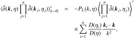 (1)where the tilde denotes the Fourier transform of the fields, η is the conformal time, D(η) is the linear growth factor, the prime in ⟨ ... ⟩ ′ denotes that we factored out the Dirac factor, ⟨ ... ⟩ = ⟨ ... ⟩ ′δD( ∑ kj), and PL(k) is the linear matter power spectrum. It is worth stressing that these relations are valid even in the nonlinear regime and for biased galaxy fields
  . The right-hand side gives the squeezed limit of the (1 + n) correlation at the leading order, which scales as 1 /k. It vanishes at this order at equal times, because of the constraint associated with the Dirac factor δD( ∑ kj).
The geometrical factors (ki·k) vanish if ki ⊥ k. Indeed, the large-scale mode induces a uniform displacement along the direction of k. This has no effect on small-scale plane waves of wavenumbers ki with ki ⊥ k, as they remain identical after such a displacement. Therefore, the terms in the right-hand side of Eq. (1) must vanish in such orthogonal configurations, as we can check from the explicit expression.
The simplest relation that one can obtain from Eq. (1)is for the bispectrum with n = 2,
 (2)where we used that k2 = − k1 − k → − k1. For generality, we considered here the small-scale fields
  and
and  to be associated with biased tracers such as galaxies. The tracers associated with k1 and k2 can be different and have different bias. At equal times the right-hand side of Eq. (2) vanishes, as recalled above.
2.2. Consistency relations for momentum correlations
The density consistency relations (1) express the uniform motion of small-scale structures by large-scale modes. This simple kinematic effect vanishes for equal-time correlations of the density field, precisely because there are no distortions, while there is a nonzero effect at different times because of the motion of the small-scale structure between different times. However, as pointed out in Rizzo et al. (2016), it is possible to obtain nontrivial equal-times results by considering velocity or momentum fields, which are not only displaced but also see their amplitude affected by the large-scale mode. Let us consider the momentum p defined by  (3)where v is the peculiar velocity. Then, in the squeezed limit k → 0, the correlation between one large-scale density mode , n small-scale density modes , and m small-scale momentum modes
  can be expressed in terms of (n + m) small-scale correlations, as
 ![Mathematical equation: \begin{eqnarray} && \hspace{-0.2cm}\left \langle \tdelta(\vk,\eta) \prod_{j=1}^n \tdelta(\vk_j,\eta_j) \prod_{j=n+1}^{n+m} \tilde{\vp}(\vk_j,\eta_j) \right \rangle_{k \rightarrow 0}' = - P_{\rm L}(k,\eta) \nonumber \\ && \times~ \Biggl \lbrace\left \langle \prod_{j=1}^n \tdelta(\vk_j,\eta_j) \prod_{j=n+1}^{n+m} \tilde{\vp}(\vk_j,\eta_j) \right\rangle' \sum_{i=1}^{n+m} \frac{D(\eta_i)}{D(\eta)} \frac{\vk_i \cdot \vk}{k^2} \nonumber \\ && + \sum_{i=n+1}^{n+m} \frac{({\rm d}D/{\rm d}n)(\eta_i)}{D(\eta)} \left \langle \prod_{j=1}^n \tdelta(\vk_j,\eta_j) \prod_{j=n+1}^{i-1} \tilde{\vp}(\vk_j,\eta_j)\right . \nonumber \\ && \left .\times~ \left( \ii \frac{\vk}{k^2} [ \delta_{\rm D}(\vk_i) + \tdelta(\vk_i,\eta_i) ] \right) \prod_{j=i+1}^{n+m} \tilde{\vp}(\vk_j,\eta_j) \right \rangle' \Biggl \rbrace . \label{consistency_relation_p} \end{eqnarray}](/articles/aa/full_html/2017/10/aa30441-17/aa30441-17-eq37.png) (4)These relations are again valid in the nonlinear regime and for biased galaxy fields and
(4)These relations are again valid in the nonlinear regime and for biased galaxy fields and  . As for the density consistency relation (1), the first term vanishes at this order at equal times. The second term, however, which arises from the
  fields only, remains nonzero. This is due to the fact that involves the velocity, the amplitude of which is affected by the motion induced by the large-scale mode.
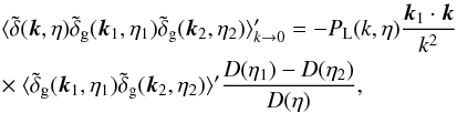
The simplest relation associated with Eq. (4)is the bispectrum among two density-contrast fields and one momentum field, 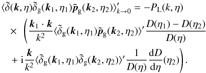 (5)For generality, we considered here the small-scale fields and
  to be associated with biased tracers such as galaxies, and the tracers associated with k1 and k2 can again be different and have different bias. At equal times, Eq. (5)reads as
 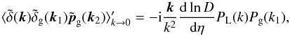 (6)where Pg(k) is the galaxy nonlinear power spectrum and we omitted the common time dependence. This result does not vanish thanks to the term generated by
  in the consistency relation (5).
2.3. Consistency relations for momentum-divergence correlations
In addition to the momentum field p, we can consider its divergence λ, defined by ![Mathematical equation: \begin{equation} \lambda \equiv \nabla \cdot \left[ (1+ \delta) \vv \right] = - \frac{\partial\delta}{\partial\eta} \cdot \label{lambda-def} \end{equation}](/articles/aa/full_html/2017/10/aa30441-17/aa30441-17-eq46.png) (7)The second equality expresses the continuity equation, that is, the conservation of matter. In the squeezed limit we obtain from Eq. (4) (Rizzo et al. 2016)
(7)The second equality expresses the continuity equation, that is, the conservation of matter. In the squeezed limit we obtain from Eq. (4) (Rizzo et al. 2016) 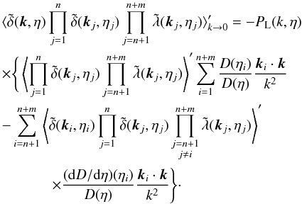 (8)These relations can actually be obtained by taking derivatives with respect to the times ηj of the density consistency relations (1), using the second equality (7). As for the momentum consistency relations (4), these relations remain valid in the nonlinear regime and for biased small-scale fields and
  . The second term in Eq. (8), which arises from the
  fields only, remains nonzero at equal times. This is due to the fact that λ involves the velocity or the time-derivative of the density, which probes the evolution between (infinitesimally close) different times.
The simplest relation associated with Eq. (8)is the bispectrum among two density-contrast fields and one momentum-divergence field, 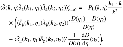 (9)At equal times, Eq. (9)reads as
 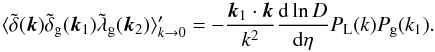 (10)
(10)
3. Observable quantities
To test cosmological scenarios with the consistency relations of large-scale structures we need to relate them to observable quantities. We describe in this section the observational probes that we consider in this paper. We use the galaxy numbers counts or the weak lensing convergence to probe the density field. To apply the momentum consistency relations (6) and (10), we use the ISW effect to probe the momentum divergence λ (more precisely the time derivative of the gravitational potential and matter density) and the kSZ effect to probe the momentum p.
3.1. Galaxy number density contrast δg
From galaxy surveys we can typically measure the galaxy density contrast within a redshift bin, smoothed with a finite-size window on the sky, ![Mathematical equation: \begin{equation} \delta_{\rm g}^{\rm s}(\vec\theta) = \int {\rm d} \vec\theta{\,'} \, W_{\Theta}(| \vec\theta{\,'} - \vec\theta |) \int {\rm d}\eta \, I_{\rm g}(\eta) \delta_{\rm g}[r, r\vec\theta{\,'} ; \eta] , \label{deltas_g-line} \end{equation}](/articles/aa/full_html/2017/10/aa30441-17/aa30441-17-eq54.png) (11)where WΘ( | θ′ − θ |) is a 2D symmetric window function centered on the direction θ on the sky, of characteristic angular radius Θ, Ig(η) is the radial weight along the line of sight associated with a normalized galaxy selection function ng(z),
(11)where WΘ( | θ′ − θ |) is a 2D symmetric window function centered on the direction θ on the sky, of characteristic angular radius Θ, Ig(η) is the radial weight along the line of sight associated with a normalized galaxy selection function ng(z),  (12)r = η0 − η is the radial comoving coordinate along the line of sight, and η0 is the conformal time today. Here and in the following we use the flat sky approximation, and θ is the 2D vector that describes the direction on the sky of a given line of sight. The superscript “s” in
  denotes that we smooth the galaxy density contrast with the finite-size window WΘ. Expanding in Fourier space, we can write the galaxy density contrast as
  (13)where k∥ and k⊥ are respectively the parallel and the perpendicular components of the 3D wavenumber k = (k∥,k⊥) (with respect to the reference direction θ = 0, and we work in the small-angle limit θ ≪ 1). Defining the 2D Fourier transform of the window WΘ as
  (14)we obtain
  (15)
(15)
3.2. Weak lensing convergence κ
From weak lensing surveys we can measure the weak lensing convergence, given in the Born approximation by ![Mathematical equation: \begin{equation} \kappa^{\rm s}(\vec\theta) = \int \!\! {\rm d}\vec\theta{\,'} W_{\Theta}(|\vec\theta{\,'}-\vec\theta|) \int \!\! {\rm d}\eta \; r \, g(r) \nabla^2 \frac{\Psi+\Phi}{2}[r,r\vec\theta{\,'};\eta] , \label{kappa-def} \end{equation}](/articles/aa/full_html/2017/10/aa30441-17/aa30441-17-eq74.png) (16)where Ψ and Φ are the Newtonian gauge gravitational potentials and the kernel g(r) that defines the radial depth of the survey is
(16)where Ψ and Φ are the Newtonian gauge gravitational potentials and the kernel g(r) that defines the radial depth of the survey is  (17)where ng(zs) is the redshift distribution of the source galaxies. Assuming no anisotropic stress, that is, Φ = Ψ, and using the Poisson equation,
  (18)where
  is the Newton constant,
  is the mean matter density of the Universe today, and a is the scale factor, we obtain
 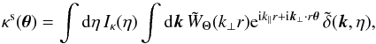 (19)with
  (20)
(20)
3.3. ISW secondary anisotropy ΔISW
From Eq. (7) λ can be obtained from the momentum divergence or from the time derivative of the density contrast. These quantities are not as directly measured from galaxy surveys as density contrasts. However, we can relate the time derivative of the density contrast to the ISW effect, which involves the time derivative of the gravitational potential. Indeed, the secondary CMB temperature anisotropy due to the integrated Sachs-Wolfe effect along the direction θ reads as (Garriga et al. 2004) ![Mathematical equation: \begin{eqnarray} \Delta_{\rm ISW}(\vec\theta) & = & \int {\rm d} \eta \, {\rm e}^{-\tau(\eta)} \left( \frac{\partial \Psi}{\partial \eta} + \frac{\partial \Phi}{\partial \eta} \right) [r,r \vec\theta;\eta] \nonumber \\[3mm] & = & 2 \int {\rm d} \eta \, {\rm e}^{-\tau(\eta)} \frac{\partial \Psi}{\partial \eta} [r,r\vec\theta;\eta] , \label{Delta-ISW} \end{eqnarray}](/articles/aa/full_html/2017/10/aa30441-17/aa30441-17-eq87.png) (21)where τ(η) is the optical depth, which takes into account the possibility of late reionization, and in the second line we assumed no anisotropic stress, that is, Φ = Ψ. We can relate ΔISW to λ through the Poisson equation (18), which reads in Fourier space as
(21)where τ(η) is the optical depth, which takes into account the possibility of late reionization, and in the second line we assumed no anisotropic stress, that is, Φ = Ψ. We can relate ΔISW to λ through the Poisson equation (18), which reads in Fourier space as  (22)This gives
  (23)where ℋ = dlna/ dη is the conformal expansion rate. Integrating the ISW effect δISW over some finite-size window on the sky, we obtain, as in Eq. (15),
  (24)with
  (25)
(25)
3.4. Kinematic SZ secondary anisotropy ΔkSZ
Thomson scattering of CMB photons off moving free electrons in the hot galactic or cluster gas generates secondary anisotropies (Sunyaev & Zeldovich 1980; Gruzinov & Hu 1998; Knox et al. 1998). The temperature perturbation, ΔkSZ = δT/T, due to this kinematic Sunyaev-Zeldovich (kSZ) effect, is 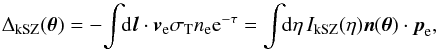 (26)where τ is again the optical depth, σT the Thomson cross section, l the radial coordinate along the line of sight, ne the number density of free electrons, ve their peculiar velocity, and n(θ) the radial unit vector pointing to the line of sight. We also defined the kSZ kernel by
  (27)and the free electrons momentum pe as
  (28)Because of the projection n·pe along the line of sight, some care must be taken when we smooth ΔkSZ(θ) over some finite-size angular window WΘ( | θ′ − θ |). Indeed, because the different lines of sight θ′ in the conical window are not perfectly parallel, if we define the longitudinal and transverse momentum components by the projection with respect to the mean line of sight n(θ) of the circular window, for example, pe ∥ = n(θ)·pe, the projection n(θ′)·pe receives contributions from both pe ∥ and pe ⊥. In the limit of small angles we could a priori neglect the contribution associated with pe ⊥, which is multiplied by an angular factor and vanishes for a zero-size window. However, for small but finite angles, we need to keep this contribution because fluctuations along the lines of sight are damped by the radial integrations and vanish in the Limber approximation, which damps the contribution associated with pe ∥.
For small angles we write at linear order n(θ) = (θx,θy,1), close to a reference direction θ = 0. Then, the integration over the angular window gives for the smoothed kSZ effect ![Mathematical equation: \begin{eqnarray} \Delta^{\rm s}_{\rm kSZ}(\vec\theta) & = & \int {\rm d}\eta \, I_{\rm kSZ}(\eta) \int {\rm d}\vk \, {\rm e}^{\ii \vk\cdot\vn r} \biggl [ \tilde{p}_{{\rm e}\parallel} \tilde{W}_{\Theta}(k_{\perp}r) \nonumber \\ && - \ii \frac{\vk_{\perp}\cdot\tilde\vp_{{\rm e}\perp}}{k_{\perp}} \tilde{W}'_{\Theta}(k_{\perp}r) \biggl ] . \;\;\; \label{kSZ-smooth} \end{eqnarray}](/articles/aa/full_html/2017/10/aa30441-17/aa30441-17-eq115.png) (29)Here we expressed the result in terms of the longitudinal and transverse components of the wave numbers and momenta with respect to the mean line of sight n(θ) of the circular window WΘ. Thus, whereas the radial unit vector is n(θ) = (θx,θy,1), we can define the transverse unit vectors as n⊥ x = (1,0, − θx) and n⊥ y = (0,1, − θy), and we write for instance k = k⊥ xn⊥ x + k⊥ yn⊥ y + k∥n. We denote
(29)Here we expressed the result in terms of the longitudinal and transverse components of the wave numbers and momenta with respect to the mean line of sight n(θ) of the circular window WΘ. Thus, whereas the radial unit vector is n(θ) = (θx,θy,1), we can define the transverse unit vectors as n⊥ x = (1,0, − θx) and n⊥ y = (0,1, − θy), and we write for instance k = k⊥ xn⊥ x + k⊥ yn⊥ y + k∥n. We denote  . The last term in Eq. (29) is due to the finite size Θ of the smoothing window, which makes the lines of sight within the conical beam not strictly parallel. It vanishes for an infinitesimal window, where WΘ(θ) = δD(θ) and
  ,
,  . We find in Sect. 5.1 that this contribution is typically negligible in the regime where the consistency relations apply, as the width of the small-scale windows is much smaller than the angular size associated with the long mode.
3.5. Comparison with some other probes
As we explained above, in order to take advantage of the consistency relations we use the ISW or kSZ effects because they involve the time-derivative of the density field or the gas velocity. The reader may then note that redshift-space distortions (RSD) also involve velocities, but previous works that studied the galaxy density field in redshift space (Creminelli et al. 2014; Kehagias et al. 2014a) found that there is no equal-time effect, as in the real-space case. Indeed, in both real space and redshift space, the long mode only generates a uniform change of coordinate (in the redshift-space case, this shift involves the radial velocity). Then, there is no effect at equal times because such uniform shifts do not produce distortions and observable signatures. In contrast, in our case there is a nonzero equal-time effect because the effect of the long mode cannot be absorbed by a simple change of coordinates. Indeed, the kSZ effect, associated with the scattering of CMB photons by free electrons in hot ionized gas (e.g., in X-ray clusters), actually probes the velocity difference between the rest-frame of the CMB and the hot gas. Thus, the CMB last-scattering surface provides a reference frame and the long mode generates a velocity difference with respect to that frame that cannot be described as a change of coordinate. This explains why the kSZ effect makes the long-mode velocity shift observable, without conflicting with the equivalence principle. There is also a nonzero effect for the ISW case, because the latter involves the time derivative of the density field, so that an equal-time statistics actually probes different-times properties of the density field (e.g., if we write the time derivative as an infinitesimal finite difference).
If we cross-correlate real-space and redshift-space quantities, there will also remain a nonzero effect at equal times, because the long mode generates different shifts for the real-space and redshift-space fields. Thus, we can consider the effect of a long mode on small-scale correlations of the weak lensing convergence κ with redshift-space galaxy density contrasts . However, weak lensing observables have broad kernels along the line of sight, so that a small differential shift along the radial direction is suppressed. In contrast, in the kSZ case the effect is directly due to the change of velocity by the long mode, and not by the indirect impact of the change of the radial redshift coordinate.
Another observable effect of the long mode was pointed out in Baldauf et al. (2015). These authors noticed that a long mode of wave length 2π/k of the same order as the baryon acoustic oscillation (BAO) scale, xBAO ~ 110h-1 Mpc, gives a different shift to galaxies separated by this distance. This produces a spread of the BAO peak, after we average over the long mode. The reason why this effect is observable is that the correlation function shows a narrow peak at the BAO scale, with a width of order ΔxBAO ~ 20h-1 Mpc. This narrow feature provides a probe of the small displacement of galaxies by the long mode, which would otherwise be negligible if the galaxy correlation were a slow power law. As noticed above, the absence of such a narrow feature suppresses the signal associated with cross-correlations among weak-lensing (real-space) quantities and redshift-space quantities, because of the radial broadening of the weak-lensing probes.
This BAO probe is actually a second-order effect, in the sense of the consistency relations. Indeed, the usual consistency relations are obtained in the large-scale limit k → 0, where the long mode generates a uniform displacement of the small-scale structures. In contrast, the spread of the BAO peak relies on the differential displacement between galaxies separated by xBAO. In the Taylor expansion of the displacement with respect to the positions of the small-scale structures, beyond the lowest-order constant term one takes into account the linear term over x, which scales as kx. This is why this effect requires that k be finite and not too small, of order k ~ 2π/xBAO.
4. Consistency relation for the ISW temperature anisotropy
In this section we consider cross correlations with the ISW effect. This allows us to apply the consistency relation (9), which involves the momentum divergence λ and remains nonzero at equal times.
4.1. Galaxy-galaxy-ISW correlation
To take advantage of the consistency relation (9), we must consider three-point correlations ξ3 (in configuration space) with one observable that involves the momentum divergence λ. Here, using the expression (24), we study the cross-correlation between two galaxy density contrasts and one ISW temperature anisotropy,  (30)The subscripts g, g1, and ISW2 denote the three lines of sight associated with the three probes. Moreover, the subscripts g and g1 recall that the two galaxy populations associated with and
  can be different and have different bias. As we recalled in Sect. 2, the consistency relations rely on the undistorted motion of small-scale structures by large-scale modes. This corresponds to the squeezed limit k → 0 in the Fourier-space Eqs. (1) and (8), which writes more precisely as
  (31)where kL is the wavenumber associated with the transition between the linear and nonlinear regimes. The first condition ensures that
  is in the linear regime, while the second condition ensures the hierarchy between the large-scale mode and the small-scale modes. In configuration space, these conditions correspond to
  (32)The first condition ensures that
  is in the linear regime, whereas the next two conditions ensure the hierarchy of scales.
The expressions (15) and (24) give 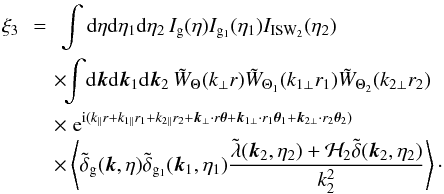 (33)The configuration-space conditions (32) ensure that we satisfy the Fourier-space conditions (31) and that we can apply the consistency relations (2) and (9). This gives
 ![Mathematical equation: \begin{eqnarray} \xi_3 = & -& \int {\rm d}\eta {\rm d}\eta_1 {\rm d}\eta_2 \, b_{\rm g}(\eta) I_{\rm g}(\eta) I_{{\rm g}_1}(\eta_1) I_{\rm ISW_2}(\eta_2) \nonumber \\ && \hspace{-0.5cm} \times \int {\rm d}\vk {\rm d}\vk_1 {\rm d}\vk_2 \, \tW_{\Theta}(k_{\perp} r) \tW_{\Theta_1}(k_{1\perp} r_1) \tW_{\Theta_2}(k_{2\perp} r_2) \nonumber \\ && \hspace{-0.5cm} \times \; {\rm e}^{\ii ( k_{\parallel} r + k_{1\parallel} r_1 + k_{2\parallel} r_2 + \vk_{\perp} \cdot r \vec\theta + \vk_{1\perp} \cdot r_1 \vec\theta_1 + \vk_{2\perp} \cdot r_2 \vec\theta_2)} \nonumber \\ && \hspace{-0.5cm} \times~ P_{\rm L}(k,\eta) \frac{\vk_1\cdot\vk}{k^2} \delta_{\rm D}(\vk+\vk_1+\vk_2) \nonumber \\ && \hspace{-0.5cm} \times~ \Biggl( \left \langle \tdelta_{{\rm g}_1} \frac{\tlambda_2 + {\cal H}_2 \tdelta_2}{k_2^2} \right \rangle' \; \frac{D(\eta_1)-D(\eta_2)}{D(\eta)} \nonumber \\[2mm] && \hspace{-0.5cm} + \left \langle \tdelta_{{\rm g}_1} \frac{\tdelta_2}{k_2^2} \right\rangle' \; \frac{1}{D(\eta)} \frac{{\rm d}D}{{\rm d}\eta}(\eta_2) \Biggl) . \label{ISW-consist-1} \end{eqnarray}](/articles/aa/full_html/2017/10/aa30441-17/aa30441-17-eq142.png) (34)Here we assumed that on large scales the galaxy bias is linear,
(34)Here we assumed that on large scales the galaxy bias is linear,  (35)where
  is a stochastic component that represents shot noise and the effect of small-scale (e.g., baryonic) physics on galaxy formation. From the decomposition (35), it is uncorrelated with the large-scale density field (Hamaus et al. 2010),
  . Then, in Eq. (34) we neglected the term
  . Indeed, the small-scale local processes within the region θ should be very weakly correlated with the density fields in the distant regions θ1 and θ2, which at leading order are only sensitive to the total mass within the large-scale region θ. Therefore, should exhibit a fast decay at low k, whereas the term in Eq. (34) associated with the consistency relation only decays as PL(k) /k ~ kns − 1 with ns ≃ 0.96. In Eq. (34), we also assumed that the galaxy bias bg goes to a constant at large scales, which is usually the case, but we could take into account a scale dependence [by keeping the factor bg(k,η) in the integral over k].
The small-scale two-point correlations ⟨ 1·2 ⟩ ′ are dominated by contributions at almost equal times, η1 ≃ η2, as different redshifts would correspond to points that are separated by several Hubble radii along the lines of sight and density correlations are negligible beyond Hubble scales. Therefore, ξ3 is dominated by the second term that does not vanish at equal times. The integrals along the lines of sight suppress the contributions from longitudinal wavelengths below the Hubble radius c/H, while the angular windows only suppress the wavelengths below the transverse radii cΘ /H. Then, for small angular windows, Θ ≪ 1, we can use Limber’s approximation, k∥ ≪ k⊥ hence k ≃ k⊥. Integrating over k∥ through the Dirac factor δD(k∥ + k1 ∥ + k2 ∥), and next over k1 ∥ and k2 ∥, we obtain the Dirac factors (2π)2δD(r1 − r)δD(r2 − r). This allows us to integrate over η1 and η2 and we obtain 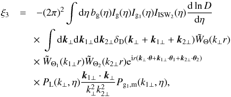 (36)where Pg1,m is the galaxy-matter power spectrum. The integration over k2 ⊥ gives
 ![Mathematical equation: \begin{eqnarray} \xi_3 & \!\! = \!\! & - (2\pi)^2 \int \!\! {\rm d}\eta \, b_{\rm g} I_{\rm g} I_{{\rm g}_1} I_{\rm ISW_2} \frac{{\rm d}\ln D}{{\rm d}\eta} \int \!\! {\rm d}\vk_{\perp} {\rm d}\vk_{1\perp} \tW_{\Theta}(k_{\perp} r) \nonumber \\[1mm] && \hspace{-0.1cm} \times~ \tW_{\Theta_1}(k_{1\perp} r) \tW_{\Theta_2}(k_{1\perp} r) P_{\rm L}(k_{\perp},\eta) P_{{\rm g}_1,{\rm m}}(k_{1\perp},\eta) \nonumber \\[1mm] && \hspace{-0.1cm} \times ~{\rm e}^{\ii r [ \vk_{\perp} \cdot (\vec\theta-\vec\theta_2) + \vk_{1\perp} \cdot (\vec\theta_1-\vec\theta_2)]} \frac{\vk_{1\perp}\cdot\vk_{\perp}}{k_{1\perp}^2 k_{\perp}^2} , \end{eqnarray}](/articles/aa/full_html/2017/10/aa30441-17/aa30441-17-eq169.png) (37)and the integration over the angles of k⊥ and k1 ⊥ gives
(37)and the integration over the angles of k⊥ and k1 ⊥ gives ![Mathematical equation: \begin{eqnarray} \xi_3 & = & \frac{(\vec\theta-\vec\theta_2) \cdot (\vec\theta_1 - \vec\theta_2)} {| \vec\theta -\vec\theta_2 | | \vec\theta_1 - \vec\theta_2 |} (2\pi)^4 \int {\rm d}\eta \, b_{\rm g} I_{\rm g} I_{{\rm g}_1} I_{\rm ISW_2} \frac{{\rm d}\ln D}{{\rm d}\eta} \nonumber \\[1mm] && \hspace{-0.1cm} \times~ \int_0^{\infty}{\rm d} k_{\perp} {\rm d} k_{1\perp} \, \tW_{\Theta}(k_{\perp} r) \tW_{\Theta_1}(k_{1\perp} r) \tW_{\Theta_2}(k_{1\perp} r) \nonumber \\[1mm] && \hspace{-0.1cm} \times~ P_{\rm L}(k_{\perp},\eta) P_{{\rm g}_1,{\rm m}}(k_{1\perp},\eta) J_1(k_{\perp} r | \vec\theta-\vec\theta_2 |) \nonumber \\[1mm] && \hspace{-0.1cm} \times~ J_1(k_{1\perp} r | \vec\theta_1-\vec\theta_2 |) , \label{xi3-J1} \end{eqnarray}](/articles/aa/full_html/2017/10/aa30441-17/aa30441-17-eq171.png) (38)where J1 is the first-order Bessel function of the first kind.
(38)where J1 is the first-order Bessel function of the first kind.
As the expression (38) arises from the kinematic consistency relations, it expresses the response of the small-scale two-point correlation  to a change of the initial condition associated with the large-scale mode . The kinematic effect given at the leading order by Eq. (38) is due to the uniform motion of the small-scale structures by the large-scale mode. This explains why the result (38) vanishes in the two following cases:
-
1.
(θ − θ2) ⊥ (θ1 − θ2). There is a nonzero response of ⟨ δ1λ2 ⟩ if there is a linear dependence on δ(θ) of ⟨ δ1λ2 ⟩, so that its first derivative is nonzero. A positive (negative) δ(θ) leads to a uniform motion at θ2 towards (away from) θ, along the direction (θ − θ2). From the point of view of θ1 and θ2, there is a reflection symmetry with respect to the axis (θ1 − θ2). For instance, if δ1> 0 the density contrast at a position θ3 typically decreases in the mean with the radius | θ3 − θ1 |, and for Δθ2 ⊥ (θ1 − θ2) the points
 are at the same distance from θ1 and have the same density contrast δ3 in the mean, with typically δ3<δ2 as
  . Therefore, the large-scale flow along (θ − θ2) leads to a positive λ2 = − Δδ2/ Δη2 independently of whether the matter moves towards or away from θ (here we took a finite deviation Δθ2). This means that the dependence of ⟨ δ1λ2 ⟩ on δ(θ) is quadratic (it does not depend on the sign of δ(θ)) and the first-order response function vanishes. Then, the leading-order contribution to ξ3 vanishes. (For infinitesimal deviation Δθ2 we have λ2 = − ∂δ2/∂η2 = 0; by this symmetry, in the mean δ2 is an extremum of the density contrast along the orthogonal direction to (θ1 − θ2).)
 -
2.
θ1 = θ2. This is a particular case of the previous configuration. Again, by symmetry from the viewpoint of δ1, the two points δ(θ2 + Δθ2) and δ(θ2 − Δθ2) are equivalent and the mean response associated with the kinematic effect vanishes.
This also explains why Eq. (38) changes sign with (θ1 − θ2) and (θ − θ2). Let us consider for simplicity the case where the three points are aligned and δ(θ) > 0, so that the large-scale flow points towards θ. We also take δ1> 0, so that in the mean the density is peaked at θ1 and decreases outwards. Let us take θ2 close to θ1, on the decreasing radial slope, and on the other side of θ1 than θ. Then, the large-scale flow moves matter at θ2 towards θ1, so that the density at θ2 at a slightly later time comes from more outward regions (with respect to the peak at θ1) with a lower density. This means that λ2 = − ∂δ2/∂η2 is positive so that ξ3> 0. This agrees with Eq. (38), as (θ − θ2)·(θ1 − θ2) > 0 in this geometry, and we assume the integrals over wavenumbers are dominated by the peaks of J1> 0. If we flip θ2 to the other side of θ1, we find on the contrary that the large-scale flow brings higher-density regions to θ2, so that we have the change of signs λ2< 0 and ξ3< 0. The same arguments explain the change of sign with (θ − θ2). In fact, it is the relative direction between (θ − θ2) and (θ1 − θ2) that matters, measured by the scalar product (θ − θ2)·(θ1 − θ2). This geometrical dependence of the leading-order contribution to ξ3 could provide a simple test of the consistency relation, without even computing the explicit expression in the right-hand side of Eq. (38).
4.2. Three-point correlation in terms of a two-point correlation
The three-point correlation ξ3 in Eq. (38) cannot be written as a product of two-point correlations because there is only one integral along the line of sight that is left. However, if the linear power spectrum PL(k,z) is already known, we may write ξ3 in terms of some two-point correlation ξ2. For instance, the small-scale cross-correlation between one galaxy density contrast and one weak lensing convergence, 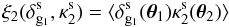 (39)reads as
 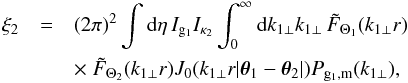 (40)where we again used Limber’s approximation. Here we denoted the angular smoothing windows by
  to distinguish ξ2 from ξ3. Then, we can write
  (41)if the angular windows of the two-point correlation are chosen such that
 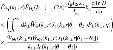 (42)This implies that the angular windows
  and
and  of the two-point correlation ξ2 have an explicit redshift dependence.
In practice, the expression (42) may not be very convenient. Then, to use the consistency relation (38) it may be more practical to first measure the power spectra PL and Pg1,m independently, at the redshifts needed for the integral along the line of sight (38), and next compare the measure of ξ3 with the expression (38) computed with these power spectra.
4.3. Lensing-lensing-ISW correlation
From Eq. (38) we can directly obtain the lensing-lensing-ISW three-point correlation,  (43)by replacing the galaxy kernels bgIg and Ig1 by the lensing convergence kernels Iκ and Iκ1,
 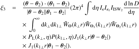 (44)As compared with Eq. (38), the advantage of the cross-correlation with the weak lensing convergence κ is that Eq. (44) involves the matter power spectrum P(k1 ⊥) instead of the more complicated galaxy-matter cross power spectrum Pg1,m(k1 ⊥).
4.4. Vanishing contribution to the galaxy-ISW-ISW correlation
In the previous section (Sect. 4.1), we considered the three-point galaxy-galaxy-ISW correlation (30), to take advantage of the momentum dependence of the ISW effect (or more precisely its dependence on the time derivative of the density field), which gives rise to consistency relations that do not vanish at equal times. The reader may wonder whether we could also use the galaxy-ISW-ISW correlation for the same purpose. From Eq. (23), this three-point correlation involves  , instead of
  in Eq. (33), where we use compact notations. Thus, we obtain the combination
 ![Mathematical equation: \begin{equation} \langle \delta \Delta_{\rm ISW_1} \Delta_{\rm ISW_2} \rangle \propto \langle \tilde\delta \tilde\lambda_1 \tilde\lambda_2 \rangle' + {\cal H} \left[ \langle \tilde\delta \tilde\lambda_1 \tilde\delta_2 \rangle' + \langle \tilde\delta \tilde\delta_1 \tilde\lambda_2 \rangle' \right] + {\cal H}^2 \langle \tilde\delta \tilde\delta_1 \tilde\delta_2 \rangle' . \label{galaxy-ISW-ISW} \end{equation}](/articles/aa/full_html/2017/10/aa30441-17/aa30441-17-eq225.png) (45)On the other hand, at equal times the consistency relation (8) writes as
(45)On the other hand, at equal times the consistency relation (8) writes as 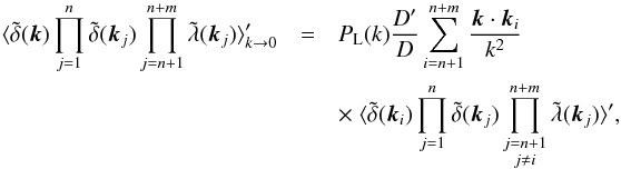 (46)where we only keep the contributions of order 1 /k and the second line in Eq. (8) cancels out. The first contribution to the three-point correlation (45) reads as
 ![Mathematical equation: \begin{eqnarray} \langle \tilde\delta \tilde\lambda_1 \tilde\lambda_2 \rangle' & = & P_{\rm L}(k) \frac{D'}{D} \left[ \frac{\vk\cdot\vk_1}{k^2} \langle \tilde\delta_1 \tilde\lambda_2 \rangle' + \frac{\vk\cdot\vk_2}{k^2} \langle \tilde\delta_2 \tilde\lambda_1 \rangle' \right] \nonumber \\ & = & P_{\rm L}(k) \frac{D'}{D} \frac{\vk\cdot\vk_1}{k^2} \left[ \langle \tilde\delta(\vk_1) \tilde\lambda(-\vk_1) \rangle' - \langle \tilde\delta(-\vk_1) \tilde\lambda(\vk_1) \rangle' \right] \nonumber \\ & = & 0 . \end{eqnarray}](/articles/aa/full_html/2017/10/aa30441-17/aa30441-17-eq227.png) (47)Here again, we only consider the leading contribution of order 1 /k and we use k2 = − k1 in the limit k → 0. The term in the bracket in the second line vanishes because the cross-power spectrum
(47)Here again, we only consider the leading contribution of order 1 /k and we use k2 = − k1 in the limit k → 0. The term in the bracket in the second line vanishes because the cross-power spectrum  only depends on | k |, because of statistical isotropy. The second contribution to Eq. (45) reads as
 ![Mathematical equation: \begin{eqnarray} \langle \tilde\delta \tilde\lambda_1 \tilde\delta_2 \rangle' + \langle \tilde\delta \tilde\delta_1 \tilde\lambda_2 \rangle' & = & P_{\rm L}(k) \frac{D'}{D} \left[ \frac{\vk\cdot\vk_1}{k^2} \langle \tilde\delta_1 \tilde\delta_2 \rangle' + \frac{\vk\cdot\vk_2}{k^2} \langle \tilde\delta_2 \tilde\delta_1 \rangle' \right] \nonumber \\ & = & 0 . \end{eqnarray}](/articles/aa/full_html/2017/10/aa30441-17/aa30441-17-eq232.png) (48)The third contribution
(48)The third contribution  vanishes as usual at equal times, as it only involves the density field. Thus, we find that the leading-order contribution to the galaxy-ISW-ISW three-point correlation vanishes, in contrast with the galaxy-galaxy-ISW three-point correlation studied in section 4.1. This is why we focus on the three-point correlations (30) and (43), with only one ISW field.
This cancellation can be understood from symmetry. Let us consider the maximal case where the points { θ,θ1,θ2 } are aligned. There is a nonzero consistency relation if the dependence of ⟨ λ1λ2 ⟩ ′ to δ(θ) contains a linear term. In the long-mode limit, this means that ⟨ λ1λ2 ⟩ ′ changes sign with the sign of the large-scale velocity flow. However, by symmetry ⟨ λ1λ2 ⟩ ′ does not select a left or right direction along the line (θ1,θ2), so that it cannot depend on the sign of the large-scale velocity flow, nor on the sign of δ(θ). In contrast, in the case of the three-point correlation (30), with only one ISW observable, the consistency relation relies on the dependence of ⟨ δ1λ2 ⟩ ′ on the large-scale mode δ (see the discussion after Eq. (38)). Then, it is clear that the nonsymmetrical quantity ⟨ δ1λ2 ⟩ ′ defines a direction along the axis (θ1,θ2), and a linear dependence on δ(θ) and on the sign of the large-scale velocity is expected.
5. Consistency relation for the kSZ effect
In this section we consider cross correlations with the kSZ effect. This allows us to apply the consistency relation (5), which involves the momentum p and remains nonzero at equal times.
5.1. Galaxy-galaxy-kSZ correlation
In a fashion similar to the galaxy-galaxy-ISW correlation studied in Sect. 4.1, we consider the three-point correlation between two galaxy density contrasts and one kSZ CMB anisotropy,  (49)in the squeezed limit given by the conditions (31) in Fourier space and (32) in configuration space. The expressions (15) and (29) give
  (50)with
 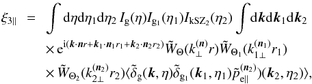 (51)and
  (52)where we split the longitudinal and transverse contributions to Eq. (29). Here { n,n1,n2 } are the radial unit vectors that point to the centers { θ,θ1,θ2 } of the three circular windows, and
  are the longitudinal and transverse wave numbers with respect to the associated central lines of sight [e.g.,
  ].
].
The computation of the transverse contribution (52) is similar to the computation of the ISW three-point correlation (34), using again Limber’s approximation. At lowest order we obtain  (53)where Pg1,e is the galaxy-free electrons cross power spectrum.
The computation of the longitudinal contribution (51) requires slightly more care. Applying the consistency relation (5) gives  (54)where we only kept the contribution that does not vanish at equal times, as it dominates the integrals along the lines of sight, and we used PL(k,η) = D(η)2PL0(k). If we approximate the three lines of sight as parallel, we can write n2·k = k∥, where the longitudinal and transverse directions coincide for the three lines of sight. Then, Limber’s approximation, which corresponds to the limit where the radial integrations have a constant weight on the infinite real axis, gives a Dirac term δD(k∥) and ξ3 ∥ = 0 (more precisely, as we recalled above Eq. (36), the radial integration gives k∥ ≲ H/c while the angular window gives k⊥ ≲ H/ (cΘ) so that k∥ ≪ k⊥). Taking into account the small angles between the different lines of sight, as for the derivation of Eq. (29), the integration over k2 through the Dirac factor gives at leading order in the angles
 ![Mathematical equation: \begin{eqnarray} \xi_{3\parallel} & = & - \!\! \int \!\! {\rm d}\eta {\rm d}\eta_1 {\rm d}\eta_2 \, b_{\rm g}(\eta) I_{\rm g}(\eta) D(\eta) I_{{\rm g}_1}(\eta_1) I_{\rm kSZ_2}(\eta_2) \frac{{\rm d}D}{{\rm d}\eta}(\eta_2) \nonumber \\ && \times \int \!\! {\rm d}k_{\parallel} {\rm d}\vk_{\perp} {\rm d}k_{1\parallel} {\rm d}\vk_{1\perp} \, \tW_{\Theta}(k_{\perp} r) \tW_{\Theta_1}(k_{1\perp} r_1) \tW_{\Theta_2}(k_{1\perp} r_2) \nonumber \\ && \times \; {\rm e}^{\ii [ k_{\parallel} (r-r_2) + \vk_{\perp} \cdot (\vec\theta-\vec\theta_2) r_2 + k_{1\parallel} (r_1-r_2) + \vk_{1\perp}\cdot (\vec\theta_1-\vec\theta_2) r_2 ]} \nonumber \\ && \times \; P_{L0}(k_{\perp}) P_{{\rm g}_1,{\rm e}}(k_{1\perp};\eta_1,\eta_2) \ii \frac{k_{\parallel}+\vk_{\perp} \cdot (\vec\theta_2-\vec\theta)}{k_{\perp}^2} \cdot \label{kSZ-consistency-2} \end{eqnarray}](/articles/aa/full_html/2017/10/aa30441-17/aa30441-17-eq256.png) (55)We used Limber’s approximation to write for instance PL0(k) ≃ PL0(k⊥), but we kept the factor k∥ in the last term, as the transverse factor k⊥·(θ2 − θ), due to the small angle between the lines of sight n and n2, is suppressed by the small angle | θ2 − θ |. We again split ξ3 ∥ over two contributions,
(55)We used Limber’s approximation to write for instance PL0(k) ≃ PL0(k⊥), but we kept the factor k∥ in the last term, as the transverse factor k⊥·(θ2 − θ), due to the small angle between the lines of sight n and n2, is suppressed by the small angle | θ2 − θ |. We again split ξ3 ∥ over two contributions,  , associated with the factors k∥ and k⊥·(θ2 − θ) of the last term. Let us first consider the contribution
  . Writing
  , we integrate by parts over η. For simplicity we assume that the galaxy selection function Ig vanishes at z = 0,
  (56)so that the boundary term at z = 0 vanishes. Then, the integrations over k∥ and k1 ∥ give a factor (2π)2δD(r − r2)δD(r1 − r2), and we can integrate over η and η1. Finally, the integration over the angles of the transverse wavenumbers yields
 ![Mathematical equation: \begin{eqnarray} \xi_{3\parallel}^{\parallel} & = & - (2\pi)^4 \int {\rm d}\eta \, \frac{{\rm d}}{{\rm d}\eta} \left[ b_{\rm g} I_{\rm g} D \right] I_{{\rm g}_1} I_{\rm kSZ_2} \frac{{\rm d}D}{{\rm d}\eta} \nonumber \\ && \times \, \int_0^{\infty} {\rm d} k_{\perp} {\rm d} k_{1\perp} \, \tW_{\Theta}(k_{\perp} r) \tW_{\Theta_1}(k_{1\perp} r) \tW_{\Theta_2}(k_{1\perp} r) \nonumber \\ && \times \, \frac{k_{1\perp}}{k_{\perp}} P_{L0}(k_{\perp}) P_{{\rm g}_1,{\rm e}}(k_{1\perp},\eta) J_0(k_{\perp} r | \vec\theta-\vec\theta_2 |) \nonumber \\ && \times\, J_0(k_{1\perp} r | \vec\theta_1-\vec\theta_2 |) , \label{xi3-kSZ-parallel} \end{eqnarray}](/articles/aa/full_html/2017/10/aa30441-17/aa30441-17-eq270.png) (57)where J0 is the zeroth-order Bessel function of the first kind. For the transverse contribution
(57)where J0 is the zeroth-order Bessel function of the first kind. For the transverse contribution  we can proceed in the same fashion, without integration by parts over η. This gives
 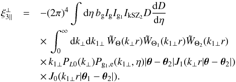 (58)It is useful to estimate the orders of magnitude of the three contributions
  , and . Using
  , and considering the case where we only have two angular scales for the angles (32),
  (59)the transverse wavenumbers are of order k⊥ ~ 1 /rΘ and ki ⊥ ~ 1 /rΘi. This gives
  (60)
(60) (61)and
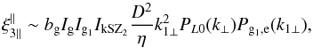
  (62)hence
  (63)Thus, we find that the contribution ξ3 ⊥ associated with the second term in Eq. (29), which is due to the angle between the lines of sight within the small conical beam of angle Θ2, is negligible as compared with the contribution ξ3 ∥ associated with the first term in Eq. (29), which is the zeroth-order term. However, the two components and are of the same order. The first one, , is the zeroth-order contribution when the lines of sight n and n2 are taken to be parallel, whereas the second one, , is the first-order contribution over this small angle, measured by | θ − θ2 | (which is, however, much larger than the width Θ2 that gives rise to ξ3 ⊥). This first-order contribution can be of the same order as the zeroth-order contribution because the latter is suppressed by the radial integration along the line of sight, which damps longitudinal modes, k∥ ≪ k⊥.
In contrast with Eq. (38), the kSZ three-point correlation, given by the sum of Eqs. (53), (57), and (58), does not vanish for orthogonal directions between the small-scale separation (θ1 − θ2) and the large-scale separation (θ − θ2). Indeed, the leading order contribution in the squeezed limit to the response of ⟨ δ1p2 ⟩ to a large-scale perturbation δ factors out as ⟨ δ1δ2 ⟩ vδ, where we only take into account the contribution that does not vanish at equal times (and we discard the finite-size smoothing effects). The intrinsic small-scale correlation ⟨ δ1δ2 ⟩ does not depend on the large-scale mode δ, whereas vδ is the almost uniform velocity due to the large-scale mode, which only depends on the direction to δ(θ) and is independent of the orientation of the small-scale mode (θ1 − θ2).
Because the measurement of the kSZ effect only probes the radial velocity of the free electrons gas along the line of sight, which is generated by density fluctuations almost parallel to the line of sight over which we integrate and which are damped by this radial integration, the result (57) is suppressed as compared with the ISW result (38) by the radial derivative dln(bgIgD) / dη ~ 1 /r. Also, the contribution (57), associated with transverse fluctuations that are almost orthogonal to the second line of sight, is suppressed as compared with the ISW result (38) by the small angle | θ − θ2 | between the two lines of sight.
One drawback of the kSZ consistency relation, (53), (57), and (58), is that it is not easy to independently measure the galaxy-free electrons power spectrum Pg1,e, which is needed if we wish to test this relation. Alternatively, Eqs. (57) and (58) may be used as a test of models for the free electrons distribution and the cross power spectrum Pg1,e.
5.2. Lensing-lensing-kSZ correlation
Again, from Eqs. (53), (57), and (58) we can directly obtain the lensing-lensing-kSZ three-point correlation,  (64)by replacing the galaxy kernels bgIg and Ig1 by the lensing convergence kernels Iκ and Iκ1. This gives
  with
with  (65)
(65)![Mathematical equation: \begin{eqnarray} \xi_{3\parallel}^{\parallel} & = & - (2\pi)^4 \int {\rm d}\eta \, \frac{{\rm d}}{{\rm d}\eta} \left[ I_{\kappa} D \right] I_{\kappa_1} I_{\rm kSZ_2} \frac{{\rm d}D}{{\rm d}\eta} \int_0^{\infty} {\rm d} k_{\perp} {\rm d} k_{1\perp} \nonumber \\ && \times \, \tW_{\Theta}(k_{\perp} r) \tW_{\Theta_1}(k_{1\perp} r) \tW_{\Theta_2}(k_{1\perp} r) \frac{k_{1\perp}}{k_{\perp}} P_{L0}(k_{\perp}) \nonumber \\ && \times\, P_{\rm m,e}(k_{1\perp},\eta) J_0(k_{\perp} r | \vec\theta-\vec\theta_2 |) J_0(k_{1\perp} r | \vec\theta_1-\vec\theta_2 |) , \label{xi3-kSZ-parallel-lens-lens} \end{eqnarray}](/articles/aa/full_html/2017/10/aa30441-17/aa30441-17-eq295.png) (66)and
(66)and  (67)This now involves the matter-free electrons cross power spectrum Pm,e.
The application of the relations above is, unfortunately, a nontrivial task in terms of observations: to test those relations one would require the mixed galaxy (matter) – free electrons power spectrum. One possibility would be to do a stacking analysis of several X-ray observations of the hot ionized gas by measuring the bremsstrahlung effect. For instance, one could infer nenpT− 1 / 2, by making some reasonable assumptions about the plasma state, as performed in Fraser-McKelvie et al. (2011), with the aim of measuring ne in filaments. We would of course need to cover a large range of scales. For kpc scales, inside galaxies and in the intergalactic medium, one could use for instance silicon emission line ratios (Kwitter & Henry 1998; Henry et al. 1996). For Mpc scales, or clusters, one may use the Sunyaev-Zeldovich (SZ) effect (Rossetti et al. 2016). Nevertheless, all these proposed approaches are quite speculative at this stage.
5.3. Suppressed contribution to the galaxy-kSZ-kSZ correlation
As for the ISW effect, we investigate whether the galaxy-kSZ-kSZ correlation provides a good probe of the consistency relations. For the same symmetry reasons as in Sect. 4.4, we find that the leading-order contribution to this three-point correlation vanishes. Let us briefly sketch how this cancellation appears. First, from the hierarchy (63) we neglect the contribution associated with the second term in Eq. (29), that is, the widths of the small-scale windows are small and we can approximate each conical beam as a cylinder (flat-sky limit). Then, we only have the component ξ3 ∥ ∥ similar to Eq. (51), which gives in compact notations ![Mathematical equation: \begin{equation} \langle \delta \Delta_{\rm kSZ_1} \Delta_{\rm kSZ_2} \rangle \propto \langle \tilde\delta(\vk) [\vn_1\cdot\tilde\vp_{\rm e}(\vk_1)] [\vn_2\cdot\tilde\vp_{\rm e}(\vk_2)] \rangle' . \end{equation}](/articles/aa/full_html/2017/10/aa30441-17/aa30441-17-eq300.png) (68)The consistency relation (4) gives at equal times
(68)The consistency relation (4) gives at equal times ![Mathematical equation: \begin{eqnarray} \langle \delta \Delta_{\rm kSZ_1} \Delta_{\rm kSZ_2} \rangle & \propto & \frac{\vn_1\cdot\vk}{k^2} \langle \tilde\delta_{\rm e}(\vk_1) [\vn_2\cdot\tilde\vp_{\rm e}(\vk_2)] \rangle' \nonumber \\ && +~ \frac{\vn_2\cdot\vk}{k^2} \langle [\vn_1\cdot\tilde\vp_{\rm e}(\vk_1)] \tilde\delta_{\rm e}(\vk_2) \rangle' . \end{eqnarray}](/articles/aa/full_html/2017/10/aa30441-17/aa30441-17-eq301.png) (69)In the regime (59), we can take n1 ≃ n2, hence
(69)In the regime (59), we can take n1 ≃ n2, hence ![Mathematical equation: \begin{eqnarray} \langle \delta \Delta_{\rm kSZ_1} \Delta_{\rm kSZ_2} \rangle & \propto & \frac{\vn_1\!\cdot\!\vk}{k^2} \vn_1 \!\cdot\! \left[ \langle \tilde\delta_{\rm e}(\vk_1) \tilde\vp_{\rm e}(-\vk_1) \rangle' + \langle \tilde\vp_{\rm e}(\vk_1) \tilde\delta_{\rm e}(-\vk_1) \rangle' \right] \nonumber \\ & = & 0 , \end{eqnarray}](/articles/aa/full_html/2017/10/aa30441-17/aa30441-17-eq303.png) (70)here we used the fact that the density-momentum cross power spectrum obeys the symmetry
(70)here we used the fact that the density-momentum cross power spectrum obeys the symmetry  , associated with a change of sign of the coordinate axis.
This cancellation can again be understood in configuration space. At leading order in the squeezed limit, the linear change of ⟨ p∥(θ1)p∥(θ2) ⟩ ′ due to a large-scale perturbation δ(θ) is (⟨ δ1p∥ 2 ⟩ ′ + ⟨ p∥ 1δ2 ⟩ ′)vδ ∥, where vδ is the large-scale velocity generated by the large-scale mode (the second-order term  does not contribute to the response function and the consistency relation). By symmetry the sum in the parenthesis vanishes. Therefore, in this paper we focus on the three-point correlations (49) and (64), with only one kSZ field.
6. Conclusions
In this paper, we have shown how to relate the large-scale consistency relations with observational probes. Assuming the standard cosmological model (more specifically, the equivalence principle and Gaussian initial conditions), nonzero equal-times consistency relations involve the cross-correlations between galaxy or matter density fields with the velocity, momentum, or time-derivative density fields. We have shown that these relations can be related to actual measurements by considering the ISW and kSZ effects, which indeed involve the time derivative of the matter density field and the free electrons momentum field. We focused on the lowest-order relations, which apply to three-point correlation functions or bispectra, because higher-order correlations are increasingly difficult to measure.
The most practical relation obtained in this paper is probably the one associated with the ISW effect, more particularly its cross-correlation with two cosmic weak-lensing convergence statistics. Indeed, it allows one to write this three-point
correlation function in terms of two matter density field power spectra (linear and nonlinear), which can be directly measured (e.g., by two-point weak lensing statistics). Moreover, the result, which is the leading-order contribution in the squeezed limit, shows a specific angular dependence as a function of the relative angular positions of the three smoothed observed statistics. Then, both the angular dependence and the quantitative prediction provide a test of the consistency relation, that is, of the equivalence principle and of primordial Gaussianity. If we consider instead the cross-correlation of the ISW effect with two galaxy density fields, we obtain a similar relation but it now involves the mixed galaxy-matter density power spectrum Pg,m and the large-scale galaxy bias bg. These two quantities can again be measured (e.g., by two-point galaxy-weak lensing statistics) and provide another test of the consistency relation.
The relations obtained with the kSZ effect are more intricate. They do not show a simple angular dependence, which would provide a simple signature, and they involve the galaxy-free electrons or matter-free electrons power spectra. These power spectra are more difficult to measure. One can estimate the free electron density in specific regions, such as filaments or clusters, through X-ray or SZ observations, or around typical structures by stacking analysis of clusters. This could provide an estimate of the free electrons cross power spectra and a check of the consistency relations. Although we can expect significant error bars, it would be interesting to check that the results remain consistent with the theoretical predictions. A violation of these consistency relations would signal either a modification of gravity on cosmological scales or non-Gaussian initial conditions. We leave to future works the derivation of the deviations associated with various nonstandard scenarios.
Acknowledgments
This work is supported in part by the French Agence Nationale de la Recherche under Grant ANR-12-BS05-0002. D.F.M. thanks the support of the Research Council of Norway.
References
- Baldauf, T., Mirbabayi, M., Simonović, M., & Zaldarriaga, M. 2015, Phys. Rev. D, 92, 043514 [NASA ADS] [CrossRef] [Google Scholar]
- Creminelli, P., Noreña, J., Simonović, M., & Vernizzi, F. 2013, J. Cosmol. Astropart. Phys., 12, 025 [CrossRef] [Google Scholar]
- Creminelli, P., Gleyzes, J., Simonović, M., & Vernizzi, F. 2014, J. Cosmol. Astropart. Phys., 2, 051 [NASA ADS] [CrossRef] [Google Scholar]
- Fraser-McKelvie, A., Pimbblet, K. A., & Lazendic, J. S. 2011, MNRAS, 415, 1961 [NASA ADS] [CrossRef] [Google Scholar]
- Garriga, J., Pogosian, L., & Vachaspati, T. 2004, Phys. Rev. D, 69, 063511 [NASA ADS] [CrossRef] [Google Scholar]
- Gruzinov, A., & Hu, W. 1998, ApJ, 508, 435 [NASA ADS] [CrossRef] [Google Scholar]
- Hamaus, N., Seljak, U., Desjacques, V., Smith, R. E., & Baldauf, T. 2010, Phys. Rev. D, 82 , 043515 [NASA ADS] [CrossRef] [Google Scholar]
- Henry, R. B. C., Kwitter, K. B., & Howard, J. W. 1996, ApJ, 458, 215 [NASA ADS] [CrossRef] [Google Scholar]
- Horn, B., Hui, L., & Xiao, X. 2014, J. Cosmol. Astropart. Phys., 9, 044 [NASA ADS] [CrossRef] [Google Scholar]
- Horn, B., Hui, L., & Xiao, X. 2015, J. Cosmol. Astropart. Phys., 9, 068 [CrossRef] [Google Scholar]
- Kehagias, A., & Riotto, A. 2013, Nucl. Phys. B, 873, 514 [NASA ADS] [CrossRef] [Google Scholar]
- Kehagias, A., Noreña, J., Perrier, H., & Riotto, A. 2014a, Nucl. Phys. B, 883, 83 [NASA ADS] [CrossRef] [Google Scholar]
- Kehagias, A., Perrier, H., & Riotto, A. 2014b, Mod. Phys. Lett. A, 29, 1450152 [NASA ADS] [CrossRef] [Google Scholar]
- Knox, L., Scoccimarro, R., & Dodelson, S. 1998, Phys. Rev. Lett., 81, 2004 [NASA ADS] [CrossRef] [Google Scholar]
- Kwitter, K. B., & Henry, R. B. C. 1998, ApJ, 493, 247 [NASA ADS] [CrossRef] [Google Scholar]
- Nishimichi, T., & Valageas, P. 2014, Phys. Rev. D, 90, 023546 [NASA ADS] [CrossRef] [Google Scholar]
- Peloso, M., & Pietroni, M. 2013, J. Cosmol. Astropart. Phys., 5, 031 [NASA ADS] [CrossRef] [Google Scholar]
- Peloso, M., & Pietroni, M. 2014, J. Cosmol. Astropart. Phys., 4, 011 [NASA ADS] [CrossRef] [Google Scholar]
- Rizzo, L. A., Mota, D. F., & Valageas, P. 2016, Phys. Rev. Lett., 117, 081301 [NASA ADS] [CrossRef] [Google Scholar]
- Rossetti, M., Gastaldello, F., Ferioli, G., et al. 2016, MNRAS, 457, 4515 [Google Scholar]
- Sunyaev, R. A., & Zeldovich, I. B. 1980, MNRAS, 190, 413 [NASA ADS] [CrossRef] [Google Scholar]
- Valageas, P. 2014a, Phys. Rev. D, 89, 123522 [NASA ADS] [CrossRef] [Google Scholar]
- Valageas, P. 2014b, Phys. Rev. D, 89, 083534 [NASA ADS] [CrossRef] [Google Scholar]
- Valageas, P., Taruya, A., & Nishimichi, T. 2017, Phys. Rev. D, 95, 023504 [NASA ADS] [CrossRef] [Google Scholar]
Current usage metrics show cumulative count of Article Views (full-text article views including HTML views, PDF and ePub downloads, according to the available data) and Abstracts Views on Vision4Press platform.
Data correspond to usage on the plateform after 2015. The current usage metrics is available 48-96 hours after online publication and is updated daily on week days.
Initial download of the metrics may take a while.