| Issue |
A&A
Volume 600, April 2017
|
|
|---|---|---|
| Article Number | A18 | |
| Number of page(s) | 16 | |
| Section | Extragalactic astronomy | |
| DOI | https://doi.org/10.1051/0004-6361/201629570 | |
| Published online | 22 March 2017 | |
Relics in galaxy clusters at high radio frequencies⋆,⋆⋆
1 Max-Planck-Institut für Radioastronomie, Auf dem Hügel 69, 53121 Bonn, Germany
e-mail: This email address is being protected from spambots. You need JavaScript enabled to view it.
2 Thüringer Landessternwarte, Sternwarte 5, 07778 Tautenburg, Germany
3 Argelander-Institüt für Astronomie, Auf dem Hügel 71, 53121 Bonn, Germany
4 Harvard-Smithsonian Center for Astrophysics, 60 Garden Street, Cambridge, MA 02138, USA
Received: 23 August 2016
Accepted: 5 December 2016
Abstract
Aims. We investigated the magnetic properties of radio relics located at the peripheries of galaxy clusters at high radio frequencies, where the emission is expected to be free of Faraday depolarization. The degree of polarization is a measure of the magnetic field compression and, hence, the Mach number. Polarization observations can also be used to confirm relic candidates.
Methods. We observed three radio relics in galaxy clusters and one radio relic candidate at 4.85 and 8.35 GHz in total emission and linearly polarized emission with the Effelsberg 100-m telescope. In addition, we observed one radio relic candidate in X-rays with the Chandra telescope. We derived maps of polarization angle, polarization degree, and Faraday rotation measures.
Results. The radio spectra of the integrated emission below 8.35 GHz can be well fitted by single power laws for all four relics. The flat spectra (spectral indices of 0.9 and 1.0) for the so-called Sausage relic in cluster CIZA J2242+53 and the so-called Toothbrush relic in cluster 1RXS 06+42 indicate that models describing the origin of relics have to include effects beyond the assumptions of diffuse shock acceleration. The spectra of the radio relics in ZwCl 0008+52 and in Abell 1612 are steep, as expected from weak shocks (Mach number ≈2.4). Polarization observations of radio relics offer a method of measuring the strength and geometry of the shock front. We find polarization degrees of more than 50% in the two prominent Mpc-sized radio relics, the Sausage and the Toothbrush, which are among the highest percentages of linear polarization detected in any extragalactic radio source to date. This is remarkable because the large beam size of the Effelsberg single-dish telescope corresponds to linear extensions of about 300 kpc at 8.35 GHz at the distances of the relics. The high degree of polarization indicates that the magnetic field vectors are almost perfectly aligned along the relic structure, as expected for shock fronts that are observed edge-on. The polarization degrees correspond to Mach numbers of >2.2. Polarized emission is also detected in the radio relics in ZwCl 0008+52 and, for the first time, in Abell 1612. The smaller sizes and lower degrees of polarizations of the latter relics indicate a weaker shock and/or an inclination between the relic and the sky plane. Abell 1612 shows a complex X-ray surface brightness distribution, indicating a recent major merger and supporting the classification of the radio emission as a radio relic. In our cluster sample, no wavelength-dependent Faraday depolarization is detected between 4.85 GHz and 8.35 GHz, except for one component of the Toothbrush relic. Faraday depolarization between 1.38 GHz and 8.35 GHz varies with distance from the center of the host cluster 1RXS 06+42, which can be explained by a decrease in electron density and/or in strength of a turbulent (or tangled) magnetic field. Faraday rotation measures show large-scale gradients along the relics, which cannot be explained by variations in the Milky Way foreground.
Conclusions. Single-dish telescopes are ideal tools to confirm relic candidates and search for new relic candidates. Measurement of the wavelength-dependent depolarization along the Toothbrush relic shows that the electron density of the intra-cluster medium (ICM) and strength of the tangled magnetic field decrease with distance from the center of the foreground cluster. Large-scale regular fields appear to be present in intergalactic space around galaxy clusters.
Key words: galaxies: clusters: general / galaxies: clusters: intracluster medium / magnetic fields / X-rays: galaxies: clusters
Based on observations with the 100-m telescope at Effelsberg, operated by the Max-Planck-Institut für Radioastronomie (MPIfR) on behalf of the Max-Planck-Gesellschaft.
The reduced Stokes parameter images (FITS files) are only available at the CDS via anonymous ftp to cdsarc.u-strasbg.fr (130.79.128.5) or via http://cdsarc.u-strasbg.fr/viz-bin/qcat?J/A+A/600/A18
© ESO, 2017
1. Introduction
Relic properties.
Radio relics are large diffuse radio sources located at the outskirts of galaxy clusters. These sources are not associated with any cluster galaxy, which can be deduced from a comparison of radio and optical observations, i.e. the large diffuse radio sources have no optical counterparts. The existence of these radio objects, observed by synchrotron emission in the radio regime, reveals the presence of relativistic electrons (and maybe a small contribution of positrons) and magnetic fields with field strengths of a few μG within the intra-cluster medium (ICM). The radio spectra (Iν ∝ ν− α) of cluster relics are steep, with spectral indices α ≥ 1, see Feretti et al. (2012) for a review.
The origin of radio relics in galaxy cluster is still a matter of debate. The present idea is that relics trace shock waves that move away from the cluster center towards regions with lower ICM density (Enßlin et al. 1998). The shocks result from mergers of galaxy clusters, which are predicted in the hierarchical model of structure formation. Radio relics that are modeled in cosmological cluster merger simulations nicely reproduce many features of observed radio relics (Hoeft et al. 2008; Skillman et al. 2011; Vazza et al. 2012; Hong et al. 2015). Several radio relics are reported as being polarized, some with a very high polarization fraction above 50% (Bonafede et al. 2009; van Weeren et al. 2010, 2011c, 2012; Kale et al. 2012; Lindner et al. 2014; de Gasperin et al. 2015). The high degree of polarization could originate from a large-scale regular magnetic field or from the compression of a small-scale tangled field in the shock front, which aligns the magnetic field lines along the structure of the shock (Laing 1980). Relics with a high fractional polarization typically show polarization vectors1 perpendicular to the relic shape, a fact readily explained via shock compression (Enßlin et al. 1998). In shock waves, the particles can be continuously accelerated via diffusive shock acceleration (DSA), which gives rise to a straight and steep radio spectrum (see Marcowith et al. (2016) for a recent review). On the other hand, Stroe et al. (2016) find evidence for spectral breaks in the two most prominent cluster relics, the so-called Sausage and Toothbrush. A break in the spectrum would indicate a more complicated origin of the relativistic electrons, for example re-acceleration of aged seed electrons (e.g., Markevitch et al. 2005), or a significant increase of the downstream magnetic field strength within the cooling time of cosmic-ray electrons (CREs; Donnert et al. 2016).
The steep spectra of radio relics hampers the detection of polarized emission at high frequencies. On the other hand, radio relics are known to have high degrees of polarization, which makes them perfect targets to study their polarization and magnetic field properties at high radio frequencies, where the effect of Faraday depolarization is small. As high-frequency observations with synthesis radio telescopes suffer from missing short spacings, which reduces the visibility of extended emission, single-dish telescopes are therefore preferable.
We observed three radio relics and one relic candidate with the Effelsberg 100-m single-dish radio telescope at two high radio frequencies, namely at 8.35 GHz (λ3.6 cm) and 4.85 GHz (λ6.2 cm). The slope of the radio spectrum of the integrated emission and the average degree of polarization are used as independent measures of the Mach numbers in the shock fronts of the relics. We measured the Faraday rotation between the two Effelsberg frequencies and we investigated the depolarization between 8.35 GHz (Effelsberg) and 1.38 GHz (Westerbork), to obtain information on the distribution of magnetic fields and ionized gas in front of the relics (i.e. the ICM and/or the Milky Way). General information on the observed relics is summarized in Table 1.
The layout of this paper is as follows. An overview of the observations and data reduction is given in Sect. 2. The results obtained from the spectral index, polarization, Faraday depolarization, and Faraday rotation data, and estimates of the magnetic field strengths in the relics are described in Sect. 3, followed by conclusions and discussion in Sect. 4. Throughout this paper, we assume a cosmology of H0 = 69 km s-1 Mpc-1, ΩM = 0.3 and Ωλ = 0.7.
2. Observations and data reduction
The radio continuum observations were performed with the Effelsberg 100-m telescope in October/November 2010, January 2011, October 2011, and August 2014, using the λ3.6 cm (8.35 GHz with 1.1 GHz bandwidth) single-horn and λ6.2 cm (4.85 GHz with 0.5 GHz bandwidth) dual-horn receiving systems, providing data channels in Stokes I, U, and Q for each horn. We used a digital broadband polarimeter as backend. The radio sources 3C 48, 3C 138, 3C 147, 3C 286, and 3C 295 were observed as flux density and pointing calibrators, using the flux densities from Peng et al. (2000). We adopted polarization angles of − 11° and + 33° for 3C 138 and 3C 286, respectively (Perley & Butler 2013). At 8.35 GHz, the maps were scanned alternating in RA and Dec directions, at 4.85 GHz in azimuthal direction only. The main part of data reduction, combining the scans into a map and subtracting the baselevels, was accomplished using the NOD2-based software package (Haslam 1974). Thereby each map in I, U, and Q was corrected for severe scanning effects, radio frequency interference (RFI) and incorrect baselevels. The dual-horn maps at 4.85 GHz were combined using software beam-switching (Emerson et al. 1979) and transformed into the RA, Dec coordinate system. The level of instrumental polarization in Effelsberg observations is below 1% and was not corrected for. All maps in Stokes parameters I, U, and Q were averaged and combined using the basket-weaving method (Emerson & Gräve 1988). The final maps were smoothed by about 10% from, originally, 82′′ to 90′′ (1.50′) at 8.35 GHz and from, originally, 146′′ to 159′′ (2.65′) at 4.85 GHz.
8.35 GHz observations.
4.85 GHz observations.
A summary of the radio observations is given in Tables 2 and 3. The rms noise in the maps of U and Q are similar, so that only the average value is given. The rms noise in the U and Q maps is several times lower than that in Stokes I because (a) the total intensity is much more affected by scanning effects owing to clouds and (b) the confusion level of weak sources is reached in most Stokes I maps, while the confusion level in U and Q is at least one order of magnitude lower and is not reached by our observations.
The astronomical image processing system (AIPS) was used to compute the radio continuum maps with respect to polarization and magnetic fields properties (i.e. polarized intensity, degree of polarization, polarization angle, and Faraday rotation). The polarized intensity was corrected for positive bias that was due to noise (Wardle & Kronberg 1974) using the option POLC in the task COMB. Since the noise distribution in the maps of polarized intensity is non-Gaussian, no rms noise values can be given, and the same rms noise levels as those in Stokes U and Q are adopted.
We also observed Abell 1612 in X-rays with Chandra for 29 ks (ObsID 15190) with ACIS-I. The data were reduced with the CIAO task chav, following the process explained in Vikhlinin et al. (2005). We used the CALDB 4.7 calibration files. Periods with high background rates and readout artifacts were removed from the data. The data were corrected for the time dependence of the charge transfer inefficiency and gain. We then subtracted the background, using the standard blank sky background files, and made a exposure corrected image in the 0.5–2.0 keV band, using a pixel binning of 4 (i.e., 2′′ pixel-1).
3. Results
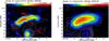 |
Fig. 1 Polarized emission (color) of the Sausage relic in CIZA J2242+53, overlaid with total intensity contours. Vectors depict the polarization B–vectors, not corrected for Faraday rotation, with lengths representing the degree of polarization. Left: 8.35 GHz map. Total intensity contours are drawn at levels of [1, 2, 3, 4, 6, 8, 16] × 1.2 mJy/beam. A vector length of 1′ corresponds to 90% fractional polarization. The beam size is 90″ × 90″. The sources are labeled according to Stroe et al. (2013). Right: 4.85 GHz map. Total intensity contours are drawn at levels of [1, 2, 3, 4, 6, 8, 16] × 2.4 mJy/beam. A vector length of 1′ corresponds to 50% fractional polarization. The beam size is 159″ × 159″. |
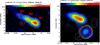 |
Fig. 2 Polarized emission (color) of the Toothbrush relic in 1RXS 06+42, overlaid with total intensity contours. Vectors depict the polarization B–vectors, not corrected for Faraday rotation, with lengths representing the degree of polarization. Left: 8.35 GHz map. Total intensity contours are drawn at levels of [1, 2, 3, 4, 6, 8, 16] × 1.5 mJy/beam. A vector length of 1′ corresponds to 90% fractional polarization. The beam size is 90″ × 90″. The sources are labeled according to van Weeren et al. (2012). Right: 4.85 GHz map. Total intensity contours are drawn at levels of [1, 2, 3, 4, 6, 8, 16] × 3 mJy/beam. A vector length of 1′ corresponds to 30% fractional polarization. The beam size is 159″ × 159″. |
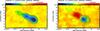 |
Fig. 3 Polarized emission (color) of the Toothbrush relic 1RXS 06+42 at 8.35 GHz in Stokes U (left) and Stokes Q (right), overlaid with total intensity contours. Vectors depict the polarization B–vectors, not corrected for Faraday rotation, with lengths representing the polarized intensity. (1′ ≡ 3 mJy/beam). Total intensity contours are drawn at levels of [1, 2, 3, 4, 6, 8, 16] × 1.5 mJy/beam. The beam size is 90″ × 90″. |
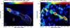 |
Fig. 4 Polarized emission (color) of the Toothbrush relic in 1RXS 06+42, overlaid with total intensity contours, from observations at the Westerbork Radio Synthesis Telescope (WSRT) (van Weeren et al. 2012). Vectors depict the polarization B–vectors, not corrected for Faraday rotation, with lengths representing the degree of polarization. The beam size is 22″ × 34″. Left: 1.38 GHz map. Total intensity contours are drawn at levels of [1, 2, 4, 6, 8, 16, 32] × 1 mJy/beam. A vector length of 1′ corresponds to 20% fractional polarization. Right: 4.9 GHz map. Total intensity contours are drawn at levels of [1, 2, 4, 6, 8, 16, 32] × 1 mJy/beam. A vector length of 1′ corresponds to 75% fractional polarization. The rms noise increases with increasing distance from the center of the primary beam which is obvious at the eastern edge of the map. |
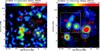 |
Fig. 5 Polarized emission (color) of the radio relic in ZwCl 0008+52, overlaid with total intensity contours. Vectors depict the polarization B–vectors, not corrected for Faraday rotation, with lengths representing the degree of polarization. The sources are labeled according to van Weeren et al. (2011c). Left: 8.35 GHz map. Total intensity contours are drawn at levels of [1, 2, 3, 4, 6, 8, 16] × 0.6 mJy/beam. A vector length of 1′ corresponds to 50% fractional polarization. The beam size is 90″ × 90″. Right: 4.85 GHz map. Total intensity contours are drawn at levels of [1, 2, 3, 4, 6, 8, 16] × 2.25 mJy/beam. A vector length of 1′ corresponds to 30% fractional polarization. The beam size is 159″ × 159″. – Note that the map area of the 8.35 GHz measurement (left panel) only includes a small region around the eastern relic (white box in the right panel), whereas the map of the 4.85 GHz measurement (right panel) encompasses the entire cluster. |
The radio continuum images of the four clusters are presented in Figs. 1–6. In all figures, the lowest contour of total intensity is plotted at the level of 3 times the rms noise in Stokes I. Significant polarized emission is detected in all clusters. The polarization vectors (rotated by 90°) are plotted only if the intensities are above three times the average rms noise in Stokes I, U, and Q.
The orientations of the polarization vectors are rotated by 90° to show the approximate orientations of the magnetic field component in the plane of the sky. The length of the vectors corresponds to the fractional polarization. Faraday rotation is not corrected in Figs. 1–6, to show the amount of rotation between the two frequencies. For Faraday rotation measures (RMs) of | RM | < 200 rad m-2 (see Fig. 14), the absolute value of the Faraday rotation angle is smaller than ±45° at 4.85 GHz and smaller than ±15° at 8.35 GHz.
3.1. CIZA J2242+53 (Sausage)
In the galaxy cluster CIZA J2242+53, van Weeren et al. (2010) detected a 2 Mpc-sized radio relic which is located in the northern outskirts of the cluster. The X-ray surface brightness distribution clearly shows that the cluster is undergoing a merger (Voges et al. 1999; Ogrean et al. 2013a, 2014). The 8.35 GHz and 4.85 GHz images of the relic obtained in this work are shown in Fig. 1. The sources are labeled according to Stroe et al. (2013). Here we show the large radio relic (RN) in the northern outskirts of the galaxy cluster. The bright point-like source seen in the bottom part of the images (C+D) is a bright head-tail radio galaxy, which is hosted by an elliptical galaxy. The source located east of the relic (H) has a much higher surface brightness than the relic and is also a tailed radio galaxy (Stroe et al. 2013). The diffuse emission seen in total intensity south of the relic is probably an artifact of the inhomogeneous baselevel (see Sect. 3.5). Comparison of total (contours) and polarized intensity (color scale) of the image at 8.35 GHz with better resolution (Fig. 1 left) implies that the point source at the eastern end of the relic (H) is not polarized and hence not part of the relic.
The magnetic field vectors show a well defined pattern aligned along the relic (RN). This indicates that the magnetic field component in the plane of the sky within the relic is well ordered, presumably because turbulent magnetic fields became anisotropic by the merger shock (see Sect. 3.7). The degree of polarization at 8.35 GHz decreases from about ≈55% at the eastern end of the relic to about ≈25% at the western end (Fig. 11 left), similar to the polarization fraction measured at 1.4 GHz by van Weeren et al. (2010) with a much higher angular resolution of 5.2″ × 5.1″. This suggests that (1) the magnetic field is ordered (anisotropic) on scales larger than the Effelsberg beam (corresponding to about 300 kpc at 8.35 GHz for this relic); and (2) wavelength-dependent Faraday depolarization in the cluster medium in front of the relic plays an insicnitifant role at these frequencies, in contrast to the Toothbrush relic (see Chap. 3.8).
The average degree of linear polarization in the eastern part is 53 ± 13%. The value is taken from the mean of all pixels in an area of about one beam and the error from the rms noise of the images in polarized and total intensity. This is among the highest values measured in radio sources, comparable to the highly polarized shock fronts of old supernova remnants (e.g. Xu et al. 2007). Feretti et al. (1998), using the Effelsberg telescope, showed that linear polarization levels of 50% are common in tailed radio galaxies. Similar levels have also been observed in the lobes of giant radio galaxies, e.g. NGC 6251 (Mack et al. 1996). More recently, Murgia et al. (2016), using the Sardinia Radio Telescope, measured a polarization level as high as 70% at 6.6 GHz in the head-tail radio galaxy 3C 129.
The degrees of polarization measured in our Effelsberg maps at 8.35 GHz and 4.85 GHz at 159′′ resolution are similar. The maximum degree of polarization is about 45%, less than at 90″ resolution because the curvature of the relic’s magnetic field within the large beam may lead to depolarization.
3.2. 1RXS 06+42 (Toothbrush)
Some characteristics of the famous Toothbrush radio relic in the galaxy cluster 1RXS06+42 are summarized in van Weeren et al. (2012, 2016): The large bright radio source has a largest linear size (LLS) of 1.87 Mpc (Table 1). The source is known to be polarized and the spectral index gradient expected for radio relics has been clearly observed for the Toothbrush, justifying the classification of the source as a relic. Enigmatically, the relic does not follow the X-ray surface brightness but extends into a region with very low ICM density towards the east. A similar behavior was also observed in the spectacular giant radio relic hosted in the double X-ray peak galaxy cluster Abel 115 (i.e. Botteon et al. 2016).
Figure 2 shows the 8.35 GHz and 4.85 GHz images of the Toothbrush radio relic obtained in this work. The 8.35 GHz image shows only the upper part of the galaxy cluster with the bright extended radio relic. The 4.85 GHz image shows a larger region around the relic including a strong background source in the south-west part of the cluster. According to observations with higher resolution by van Weeren et al. (2012), shown in Fig. 4, the relic consists of a bright western part and a fainter linear extension to the northeast, which is also seen in the Effelsberg images. The relic apparently comprises three components. Following van Weeren et al. (2012), we label the components B1−B3 (see Fig. 2).
Our measurements show that the relic is polarized over its entire length. The polarization fraction at 8.35 GHz at 90″ resolution, see Fig. 11 right panel, strongly varies along the relic, with 30 ± 8% in region B3, a maximum of 45 ± 7% in region B2, and 15 ± 1% in region B1. Our results of the degrees of polarization for all three components are similar to those obtained with the WSRT at 4.9 GHz by van Weeren et al. (2012), see Fig. 4 right panel. The WSRT observations show that region B3 is polarized at 1.38 GHz (Fig. 4 left panel) at a similar level (≃32 ± 4%) as obtained from the Effelsberg observations at 8.35 GHz, while regions B2 and B1 have significantly less polarization at 1.38 GHz compared to the higher frequencies (see Sect. 3.8).
The orientations of the magnetic field lines are changing along the relic, which is unexpected for a continuous shock front. This is best demonstrated by the maps in Stokes U and Q (Fig. 3). While the map in Stokes U shows a smooth distribution, two components are clearly separated in the map in Stokes Q that can be identified as B1 and B2+B3. The internal structure of the shock front or Faraday rotation in the foreground are possible reasons (see Sect. 3.9).
3.3. ZwCl 0008+52
On the east side of the galaxy cluster ZwCl 0008+52, van Weeren et al. (2011c) find a large arc of diffuse radio emission. Based on the location with respect to the cluster center (determined through X-ray observations) and the morphology, they classify the radio source as a radio relic. Furthermore, they do not find any optical counterparts to the diffuse emission, which suggests that the emission is not connected to any cluster galaxy.
The 8.35 GHz and 4.85 GHz images of the relic from our observations are shown in Fig. 5. We note that the map area of the 8.35 GHz measurement (left panel) only includes a small region around the eastern relic (indicated by the dashed box in the right panel), whereas the map of the 4.85 GHz measurement encompasses the entire cluster, including four bright and polarized radio galaxies (named A, B, C, and E/F by van Weeren et al. 2011c). The eastern radio relic (RE) can be seen in both images, but only the southern part of the relic is clearly detected at 8.35 GHz. At 4.85 GHz, polarized emission is detected along the whole extent of the relic with the B–vectors aligned, while the high-resolution observations of van Weeren et al. (2011c) at 1.38 GHz showed only a few small spots of polarized emission. The western relic cannot be separated from the western radio galaxies in our map at 4.85 GHz.
A maximum degree of polarization of ≃25% (at 1.38 GHz) for the eastern relic is reported by van Weeren et al. (2011c). Our results show that the relic is polarized with a varying degree of polarization, with a maximum in the southern part of 26 ± 7% at 8.35 GHz and 22 ± 4% at 4.85 GHz, while the northern part has a lower degree of polarization of 13 ± 3% at 4.85 GHz.
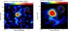 |
Fig. 6 Polarized emission (color) of the radio relic in Abell 1612, overlaid with total intensity contours. Vectors depict the polarization B–vectors, not corrected for Faraday rotation, with lengths representing the degree of polarization. Left: 8.35 GHz map. Total intensity contours are drawn at levels of [1, 2, 3, 4, 6, 8, 16] × 1.5 mJy/beam. A vector length of 1′ corresponds to 30% fractional polarization. The beam size is 90″ × 90″. Right: 4.85 GHz map. Total intensity contours are drawn at levels of [1, 2, 3, 4, 6, 8, 16] × 1.5 mJy/beam. A vector length of 1′ corresponds to 20% fractional polarization. The beam size is 159″ × 159″. |
The measurements show that most of the polarization B −vectors are aligned parallel to the major axis of the relic. Nevertheless, further observations are needed to better map the polarization properties. Especially, further polarization observations at 8.35 GHz are needed with a larger map area and higher sensitivity to detect the western relic and fully trace the eastern relic.
3.4. Abell 1612
An elongated radio source located in the southern outskirts of the galaxy cluster Abell 1612 is examined by van Weeren et al. (2011b). To the north of the extended radio emission there is a bright, tailed radio galaxy. The authors classify the elongated radio source as a candidate for a radio relic because it is apparently not connected to the radio galaxy and they cannot find any optical counterpart for the radio source.
The images shown in Fig. 6 present the southern part of the galaxy cluster with a bright radio galaxy in the center (A) and the relic candidate on the southern side (R). Owing to the large beam sizes of our observations, the detailed structure of the southern relic is smeared out.
We subtracted bright sources from the Chandra X-ray image and smoothed the image to a beam size of 30″ × 30″, to reveal the diffuse X-ray emission, see Fig. 7. The two bright radio sources both have optical counterparts with SDSS spectroscopic redshifts, consistent with them being cluster members. The counterparts are massive elliptical galaxies.
The Chandra image displays a clumpy morphology for the distribution of the ICM. The X-ray concentrations near the two radio sources seem to belong to two different subclusters with distinct cD galaxies as judged from optical William Herschel Telescope (WHT) imaging, see Fig. 8. The structures are separated by about 5 arcmin, which corresponds to about 900 kpc. The brighter X-ray emission between the two subclusters likely originates from ram-pressure stripped gas left after the core passage of the two subclusters. Additional X-ray emission extends to the north that could be from a third merging substructure.
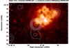 |
Fig. 7 X-ray emission (color) of Abell 1612 taken with Chandra and smoothed to a beam size of 30″ × 30″, overlaid with contours of total radio emission at 8.35 GHz with a beam size of 90″ × 90″. Contours are drawn at levels of [1, 2, 3, 4, 6, 8, 16] × 1.5 mJy/beam. |
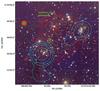 |
Fig. 8 Overlay of a WHT image of Abell 1612 with the X-ray surface brightness (red-yellow contours) and the total radio emission at 8.35 GHz (blue contours). |
The X-ray surface brightness clearly shows a recent merger of the galaxy cluster. According to the X-ray morphology a large merger shock could be present at the position of the radio relic. Evidently, the relic is asymmetrically located to the merger axis defined as by the two cD galaxies. Other radio relics are asymmetric with respect to the merger axis as well, see for example the relic in the complex merging cluster Abell 115 (Govoni et al. 2001; Botteon et al. 2016). The Toothbrush relic is also asymmetric to the main merger axis. Brüggen et al. (2012) suggest a triple merger for the origin. Similarly, the merger in Abell 1612 apparently comprises several subcomponents.
To determine the global cluster temperature, we extracted a spectrum in a circular region of 1 Mpc radius, centered on RA = 12h47m43s.8, Dec = −02° 48′ 00″. We fitted this spectrum with XSPEC (v12.9), fixing the redshift to z = 0.179, the abundance to 0.25, and NH = 1.82 × 1020 cm-2 (the weighted average NH from the Leiden/Argentine/Bonn (LAB) survey, Kalberla et al. 2005). Regions contaminated by compact sources were excluded from the fitting. From this fit, we find a temperature of  keV and a 0.1–2.4 keV rest-frame luminosity of 1.8 × 1044 erg s-1.
In Abell 1612, no polarization had been detected prior to this work. Our measurements reveal significant polarized emission at 8.35 GHz. The polarization degree at 8.35 GHz is 20 ± 7% at RA ≃ 12h47m56s, Dec ≃ −02° 52′. The polarization degree at 4.85 GHz cannot be measured with sufficient accuracy because the relic is too close to the central radio galaxy (A). The extensions of polarized emission toward RA ≃ 12h47m55s, Dec ≃ −02° 54′ at 8.35 GHz and toward RA ≃ 12h47m43s, Dec ≃ −02° 55′ at 4.85 GHz are at the level of 2.5 times the rms noise and therefore probably not real.
The high angular resolution images obtained by (van Weeren et al. 2011b; their Fig. 2), as well as the fact that these authors did not find any optical counterpart of the elongated radio source in Abell 1612 and our significant detection of polarization, confirm that this radio source is indeed a radio relic.
3.5. Integrated flux densities and spectral indices
Flux densities of point sources.
Integrated flux densities and fractional polarizations.
The integrated flux densities in total and polarized intensity were obtained by integrating within 1σ (Table 5). We thereby defined different integration areas around the relic down to the noise level for all relics and both frequencies (see Tables 2 and 3).
To correct the baselevel of each map in Stokes I, U, and Q, the mean intensity of each map was measured by selecting at least five boxes (each containing about one beam size) in regions where no emission from sources is detected. The average of these values was subtracted from the final map. Since the sizes of some maps are too small to find a sufficiently large number of regions without signal, the uncertainties in the baselevel subtraction are quite large and affect the integrated flux densities. Furthermore, for the same reason, the baselevels may not be homogeneous (large-scale fluctuations) in the maps, which leaves artifacts in total and polarized intensity.
The point sources external to the Sausage relic, named B and H by Stroe et al. (2013), and the source F external to the Toothbrush relic (see Figs. 1 left and 2 left) were subtracted from maps of the total intensity at 8.35 GHz before performing the integration. As these three sources are not resolved at 4.85 GHz, we extrapolated their flux densities from 8.35 GHz by assuming a spectral index of 1.0. The resulting additional error in the integrated flux density at 4.85 GHz is much smaller than the error due to the baselevel uncertainty (see above). For Abell 1612, the bright source north of the relic (A) was subtracted from the maps before performing the integration. The flux densities of the subtracted point sources are given in Table 4. For ZwCl 0008+52, no point sources had to be subtracted.
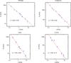 |
Fig. 9 Integrated total intensity spectra of the relics considered in this paper. Top left: spectrum of the Sausage radio relic. The flux densities at frequencies lower than 4.85 GHz are taken from Table 3 of Stroe et al. (2016). Top right: spectrum of the Toothbrush radio relic. The flux densities at frequencies lower than 4.85 GHz are taken from Table 3 of Stroe et al. (2016). Bottom left: spectrum of the radio relic in ZwCl 0008+52. The flux densities at frequencies lower than 4.85 GHz are taken from van Weeren et al. (2011c). Bottom right: spectrum of the radio relic in Abell 1612. The flux densities at frequencies lower than 4.85 GHz are taken from van Weeren et al. (2011b). |
The uncertainty of the flux density measurements is dominated by the uncertainty in the baselevel of a map. The uncertainties owing to rms noise in a map and the uncertainties in the procedure of source subtraction are much smaller and can be ignored. The absolute calibration error of about 5% affects all flux densities in the same way and is disregarded in the following.
To obtain the uncertainty Δs of a flux density measurement, we determined the standard deviation σs of the mean intensities of the boxes, where the baselevel was measured. As this uncertainty systematically affects the flux density of the source, we multiplied σs with the number of beams Nbeam within the integration area:  (1)This equation is applicable if the scale of the fluctuations in the baselevel is larger than the size of the integration area, while smaller-scale fluctuations would be cancelled out in the integration process.
The plotted spectra for all relics considered in this paper are shown in Fig. 9. We decided to use the flux densities at frequencies below 4.85 GHz from Table 3 of Stroe et al. (2016), which were obtained from images from uv data beyond 800 λ, corresponding to angular scales of smaller than about 3′. The reasons are the following: (1) The Sausage relic shows diffuse extended emission at 153 MHz but not at higher frequencies (Stroe et al. 2013), indicating that this emission has a steep spectrum. Hence little additional emission is expected when using images based on uv data smaller than 800 λ. However, the flux densities in Table 4 of Stroe et al. (2016) are higher by factors of 1.4–2.1 than those in Table 3 of Stroe et al. (2016). (2) The flux density of the Toothbrush relic at 1.4 GHz in Table 3 agrees well with that at 1.5 GHz by van Weeren et al. (2016), based on JVLA D-array data that hardly suffer from missing large-scale emission.
For all four relics, we find flux densities which are in accordance with power law distributions at frequencies below 4.85 GHz. We do not find any evidence for significant spectral steepening at frequencies below 8.35 GHz in any of the four relics. This also rules out a significant B-field variation within the CRE cooling time. The steepening found by Stroe et al. (2016) for the Sausage and Toothbrush relics are based on two values at higher frequencies that, however, have large errors and may suffer from the SZ effect (Basu et al. 2016). We note that the integrated flux densities of the Sausage and Toothbrush relics given in Table 4 of Stroe et al. (2016) are based on the same maps as in this work, but are slightly different because the values in our Table 5 are obtained with somewhat different integration areas and an additional source subtraction in the case of the Toothbrush relic.
The flux density of the Toothbrush relic at 4.85 GHz in Table 5 is possibly too low compared to 8.35 GHz and the values at lower frequencies (Fig. 9). The probable reason is the insufficient size and low quality of this map. Interestingly, our results indicate that the radio spectrum of the Toothbrush runs up to 8.35 GHz with a constant spectral index of about 1.0. In X-rays, only a moderately strong shock has been reported, with a Mach number of about 1.5 (Itahana et al. 2015; van Weeren et al. 2016).
According to diffusive shock acceleration (DSA) theory in the test particle regime, particles get accelerated at a shock front to relativistic energies that show a power law distribution in particle energy (Blandford & Eichler 1987). The strength of the shock, described by the Mach number or the compression ratio, determines the exponent, sinj, of the energy spectrum. Radio relics are straightforwardly explained with DSA: The merger shock injects CREs into the ICM. While the shock front propagates further out, the CREs cool. If the shock properties do not change on a time scale comparable to the cooling time of the CREs that generate the observed synchrotron emission, the CRE energy distribution is in steady-state, determined by continuous injection and synchrotron and inverse Compton (IC) losses. The resulting overall CRE energy spectrum is again a power law (N(E) ∝ E− s) with s = sinj + 1 (e.g. Sarazin 1999). The overall radio spectrum is therefore a power law as well. The spectral index α of the spectrum of flux densities integrated over the relic (see Table 5) is related to the Mach number ℳ according to 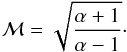 (2)Evidently, in the DSA scenario the radio spectrum is a power law with spectral index steeper than 1. A bent spectrum is obtained, for instance in the case of re-acceleration of a pre-existing mildly relativistic electron population or with a variable downstream magnetic field strength (Donnert et al. 2016). We found spectral indices of 0.90 ± 0.04 and 1.00 ± 0.04 for the Sausage and the Toothbrush, respectively, indicating that models that describe the origin of relics have to include effects beyond the assumptions made above. For instance, if the Mach number and the injection electron spectrum change on timescales comparable to the cooling time, the steady-state assumption is violated and the resulting spectrum may deviate from Eq. (2). Measuring the spectral index close to the shock front with high angular resolution provides a more reliable estimate for the injection spectrum.
We note that, for the Toothbrush only, a moderately strong shock has been reported from X-ray observations, with a Mach number of about 1.5 (Itahana et al. 2015; van Weeren et al. 2016). According to Eq. (2) this corresponds to a spectral index of 2.6, which is evidently not in accord with the observations. There is an ongoing debate on whether X-ray observations tend to indicate too low Mach numbers or if the acceleration mechanism is far more complex than the DSA of thermal or mildly relativistic electrons.
For the eastern relic in ZwCl 0008, we confirm a steep spectral index as reported by van Weeren et al. (2011c). The flux measurements of the relic in Abell 1612 are rather uncertain owing to the proximity of the tailed radio galaxy. In combination with flux density measured at 1.38 GHz, our measurements indicate, however, a spectral index of about 1.4. For both relics, the spectral index is rather steep compared to relics associated with merger shocks (Feretti et al. 2012). According to DSA in the test-particle regime, the spectral index corresponds to a Mach number of about 2.4.
3.6. Magnetic field strengths
Equipartition magnetic field strengths (assuming a proton-to-electron ratio of K = 100).
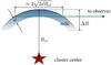 |
Fig. 10 Sketch for the path length through the emitting volume of a relic. The width of the downstream volume is given by the cooling time of the electrons. The green line indicates the line of sight with the maximum path length through the emitting volume. d is the intrinsic width and ΔR the observable width of the relic (see Table 1). For d ≪ Rcc the maximum path length can be approximated by |

The synchrotron emission from radio relics gives evidence that the intra-cluster medium in the downstream region of the shocks is significantly magnetized. About 50 radio relics have been detected so far. However, very little is known about the strength and structure of magnetic fields in relics, see Govoni & Feretti (2004) for a summary. The radio intensity alone does not provide information on the field strength without additional assumptions, since the density of relativistic electrons is not known. The most promising approach to measure the latter is to detect the IC signature of relativistic electrons in the hard X-ray band. So far, only upper limits for the IC emission have been obtained. They provide lower limits for field strength in relics when combining with the radio luminosity. For two relics, namely Abell 3667 and the Toothbrush relic, Finoguenov et al. (2010) and Itahana et al. (2015) conclude that the field strengths in the relic regions are larger than 3 μG and 1.6 μG, respectively.
One possibility to break the degeneracy between relativistic electron density and magnetic field strength is to assume energy equipartition between magnetic fields and cosmic rays (CRs). This has led to reasonable estimates for the total magnetic field strengths (Beck & Krause 2005).
Slee et al. (2001) observe radio-bright relics in four galaxy clusters and find a total field strengths of 7–14 μG from the minimum energy assumption, which gives similar results to the equipartition assumption, and adopting a proton-to-electron ratio of K = 1. However, all four relics are classified as so-called radio phoenixes, i.e. they are believed to originate from radio galaxies, possibly re-energized by shock compression (Enßlin & Gopal-Krishna 2001). Therefore, these objects likely comprise a stronger magnetic field than the relics associated with large merger shocks.
Another approach to measure the magnetic field strength in galaxy clusters is the analysis of the Faraday rotation of polarized sources in the background or embedded in the ICM. The rotation of the polarization direction measures the average line-of-sight component of the magnetic field weighted with the thermal electron density. Bonafede et al. (2013) studied the rotation measures of background sources close to the radio relic in the Coma cluster. They derived a strength of the line-of-sight field of ≥2 μG, which is basically in agreement with the lower limits and estimates as discussed above.
We apply the revised energy equipartition formula (Beck & Krause 2005) to estimate the magnetic field strength. Using this method, the CR spectrum is integrated down to E = 0, assuming a spectral break at the rest mass of the CR protons at 936 MeV, as expected for a DSA spectrum that is a power law in momentum space. If however the CR energy is dominated by leptons, the integration should be performed over the electron spectrum. As the low-energy electrons below a few 100 MeV suffer strongly from energy losses, a spectral break at 936 MeV still seems like a useful assumption and should yield reasonable equipartition values.
The strength of the total magnetic field Btot, ⊥ in the sky plane is derived from the total synchrotron intensity Isync via ![Mathematical equation: \begin{equation} B_{\mathrm{tot},\perp} \propto [I_\mathrm{sync}/(L \, (K+1))]^{\,\,\,1/(3+\alpha_{\text{inj}})} . \label{eq:equi} \end{equation}](/articles/aa/full_html/2017/04/aa29570-16/aa29570-16-eq162.png) (3)To derive field strengths, assumptions have to be made for the proton-to-electron ratio K of the number densities of CR particles in the GeV range, the path length L, and the synchrotron spectral index αinj at the location where the CRs are accelerated.
(3)To derive field strengths, assumptions have to be made for the proton-to-electron ratio K of the number densities of CR particles in the GeV range, the path length L, and the synchrotron spectral index αinj at the location where the CRs are accelerated.
The radio emission probes only the CR electron content. CR protons in galaxy clusters have not been detected, so that we can only speculate how much energy is stored in CR protons. Diffusive particle acceleration typically predicts K of the order of K = 100 (Bell 1978). However, this type of high proton-to-electron ratio may violate the upper limits from observations with the FERMI telescope (Vazza et al. 2015).
It has been recently suggested that at low Mach number shock front electrons might be scattered back and forth at the shock, as assumed for a Fermi I-type process, and gain energy via shock drift acceleration (SDA) (Guo et al. 2014a). Such a process only accelerates electrons. If electrons at merger shock fronts are accelerated by SDA, the efficiency for proton acceleration may be negligible since the Mach numbers of merger shocks are low, ℳ ≲ △, and DSA would not be efficient enough to accelerate protons, implying a proton-to-electron ratio close to K = 0. To back-scatter electrons in the upstream region, the large-scale guiding magnetic field needs to be disturbed. As shown by Guo et al. (2014b), the Firehose instability may sufficiently twist the field lines, provided that the upstream plasma has a low magnetization, i.e. the ratio of thermal to magnetic energy densities has to be large, β> 20.
In addition to K, the synchrotron spectral index α and the path length L through the synchrotron-emitting medium need to be known. The integrated α values in Table 5 represent the spectrum of cosmic-ray electrons that is steepened by synchrotron losses. Since equipartition holds for the freshly injected particles, we assume injection values of αinj = 0.7 for the Sausage relic (Stroe et al. 2013) and the Toothbrush relic (van Weeren et al. 2012). For ZwCl 0008+52 and Abell 1612 we correct α for synchrotron losses by 0.5 which gives αinj = 0.9.
The intrinsic width of a radio relic, i.e. the downstream extent of the emitting volume, can be estimated from the downstream velocity and the magnetic field strength. The velocity of the downstream plasma with respect to the shock is basically given by the downstream specific energy density (Hoeft & Brüggen 2007); for a plasma with a temperature of 7 keV the velocity amounts to about 1400 km s-1. Adopting this velocity, 66% of the emission at about 5 GHz originates from a volume within a distance of about 10 kpc to the shock front (Hoeft et al., in prep.). In observations, relics are more extended into the downstream direction, see Table 1 (Col. 8). Smoothing that is due to the resolution of the observation and projection effects (since the shock fronts may not be aligned with the line of sight) define the observed width.
Simulations from van Weeren et al. (2011a) show that a calotte of a sphere is a good approximation for the shape of a relic. Figure 10 illustrates an estimate for the path length through the emitting volume. We used this simple geometry to calculate the average path length L through the relic from the distance to the cluster center, Rcc, and the intrinsic width, d. We assume that the average path length for all lines of sight through the emitting volume of the relic is  of maximum path length, hence
 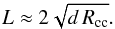 (4)Adopting 10 kpc for the intrinsic width and 1.0–1.5 Mpc for the distance to cluster center, we obtain 200–250 kpc for the average path length through the emitting volume in the four relics.
Equation (3) yields the field component Btot, ⊥ perpendicular to the line of sight, giving rise to synchrotron emission. The shock front generating the relic amplifies the field components in the plane of the shock front that is seen primarily edge-on. Hence, the field components along the relic and along the line of sight are enhanced. As synchrotron emission emerges only from the component in the sky plane, only emission from the compressed field along the relic is observed. To correct for the invisible field components along the line of sight, we require an average angle between all possible orientations of the field in the plane of the shock front and the line of sight. We assume that this angle is 45°.
Assuming L = 200 kpc and K = 100 yields total field strengths in the range 2.4–4.2 μG (Table 6). The value for the Sausage relic is consistent with the estimate of 5–7 μG derived from the width of the relic by van Weeren et al. (2010). For K = 0 all values are smaller by the factor 101−1/(3 + αinj) (see Eq. (3)) and become 0.7–1.2 μG.
The largest uncertainties of Btot emerge from the values assumed for the path length L and the ratio K. Changing one of these values by a factor a changes the field strength by a factor of a−1/(3 + α) (Eq. (3)). Owing to the simplified geometrical model of the relic shape, we estimate an uncertainty of a ≤ 3, resulting in an error in Btot of ≲30%.
The component of the magnetic field that is aligned along the shock front, called the anisotropic field Ban (see Sect. 3.7), is computed from the degree of linear polarization and is also listed in Table 6. Owing to the limited resolution of our observations, the strengths of the anisotropic field in Table 6 are lower limits and may, in fact, be very similar to the total field strengths.
Adopting a typical electron density in the cluster periphery of 10-4cm-3 (Croston et al. 2008) and a temperature of 8 keV, as found for the Toothbrush (van Weeren et al. 2016), results in a plasma–β (the ratio between the energy densities of thermal gas and magnetic fields) in the range 1.3 to 14, where the higher value corresponds to the lower field strength. It is not clear if energy equipartition or minimum energy arguments apply for the field in the downstream plasma of merger shocks. However, the considerations presented above permit a scenario in which only electrons are accelerated, i.e. K = 0, so that the lower field estimates apply, B ≈ 1μG. This value reflects the strength in the downstream regime, where the field strength is presumably higher due to compression at the shock front, or CR-induced instabilities, and/or turbulent amplification. In a much weaker upstream field (β ≳ 10), Firehose instabilities can generate upstream waves, which allow multiple energy gains of electrons, which enable a Fermi I-type process for electron acceleration at a low Mach number shock. A significantly stronger magnetic field would not permit such a process.
On the other hand, the non-detection of IC emission from the Toothbrush relic yields a lower limit for the field strength in downstream region of 1.6 μG (Itahana et al. 2015). Furthermore, Basu et al. (2016) estimate a total field strength of the Sausage relic of about 2.5 μG from the flux ratio between the Sunyaev-Zel’dovich (SZ) and the synchrotron signals and with an ad hoc assumption for the electron acceleration efficiency. Field strengths of a few μG in the downstream region correspond to a plasma–β about unity. Hence, these results favor the strong-field scenario where both protons and electrons are accelerated in the shock front.
3.7. Mach numbers derived from the degree of polarization
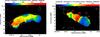 |
Fig. 11 Degree of polarization (color) of the Sausage relic (left) and the Toothbrush relic (right) at 8.35 GHz with 90″ × 90″ resolution. The contours show the polarized intensity at [1, 2, 4, 6] × 0.21 mJy/beam for the Sausage relic (left) and at [1, 2, 4, 6, 8] × 0.39 mJy/beam for the Toothbrush relic (right). |
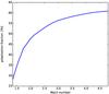 |
Fig. 12 Degree of polarization as a function of the Mach number of the shock. The polarization is derived assuming a weak upstream magnetic field that is isotropically tangled on small scales and compressed at the shock front (Hoeft et al., in prep.). |
Enßlin et al. (1998) suggested that shock fronts in the ICM induced by cluster mergers are the origin of radio relics. In the proposed scenario, electrons are accelerated at the shock front via diffusive shock acceleration. While the shock front propagates further, the relativistic electrons cool via synchrotron and IC emission. Furthermore, Enßlin et al. (1998) argue that the relics should be polarized Because of the compression of turbulent or tangled magnetic fields at the shock front, see also Laing (1980). This model can be briefly summarized as follows: The medium ahead of the shock fronts is permeated by magnetic fields that are turbulent or tangled on scales many orders of magnitude smaller than the length scale that corresponds to the telescope beam. The distribution of magnetic field vectors in the upstream medium is isotropic. Shock compression causes the magnetic field components parallel to the front to be stretched and amplified, while the perpendicular components remain constant. As a result, the magnetic field behind the shock front is still randomly tangled, but the distribution of field orientations is not isotropic anymore (also called an anisotropic field). It is stretched parallel to the plane of the shock. This causes the synchrotron emission to be polarized, depending on the degree of anisotropy caused by the shock front.
In a numerical model, described in detail in a forthcoming paper (Hoeft et al., in prep.), we study the Mach number dependence of the fractional polarization (see Fig. 12). A shock with a Mach number of 2.0 already causes a fractional polarization of about 48%. However, it should be kept in mind that this is computed for relics seen perfectly edge-on and assuming no further depolarization, for instance owing to variations in the orientation of the shock surface. Interestingly, the relics in ZwCl 0008 and Abell 1612 shows a steeper spectral index in the radio spectrum and also a lower degree of polarization, both indicating a low Mach number.
The Toothbrush relic is studied in detail by van Weeren et al. (2016). They find that the spectral index at the northern edge varies in the range  . The regions of brighter emission along the edge correlate with the regions showing a flatter spectrum. Owing to the high resolution in the images, the measured spectral index at the edge should be close to the injection spectrum. Adopting DSA implies Mach numbers in the range ℳ ≈ 2.8−3.3. Hence, the intrinsic polarization that is due to a compressed magnetic field should be about 50% to 55%. Actually, our observation shows for 8.35 GHz a polarization of about 45% for the region B2. According to Fig. 12, this implies that the minimum Mach number in that region is 2.0. However, even if the Mach number is significantly higher, the observed degree of polarization is very close to the intrinsic one, i.e. only slight depolarization is possible, for instance owing to Faraday rotation depolarization of a foreground magnetic field.
3.8. Faraday depolarization in the Toothbrush relic
Wavelength-dependent Faraday depolarization at GHz frequencies needs strong magnetic fields and/or high densities of thermal electrons (Sokoloff et al. 1998; Arshakian & Beck 2011). Strong gradients in Faraday rotation can also cause depolarization. Clear evidence for the existence of magnetic fields in the ICM comes from radio emission in radio relics and halos, while the morphology of the fields is still unknown. The polarization of radio relics could, for instance, be caused either by large-scale ordered fields or by small-scale anisotropic fields, as discussed above. The alignment of the polarization orientation (B −vectors) with the shock surface favors small-scale anisotropic (compressed) fields. Because of the small path length along the line of sight within the relic, these fields are less efficient to depolarize than large-scale fields in the ICM or in the intergalactic medium. Hence, in the following, we assume that Faraday depolarization (if any) occurs in the medium in front of the relic.
The dispersion in RM within the telescope beam, σRM, is a useful parameter to characterize Faraday depolarization (Burn 1966; Sokoloff et al. 1998; Arshakian & Beck 2011). In the case of a turbulent medium between the observer and the emitting volume, the wavelength-dependent depolarization depends on the Faraday dispersion according to 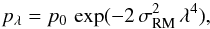 (5)where p0 is the intrinsic (wavelength-independent) degree of polarization.
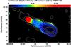 |
Fig. 13 Depolarization between 1.38 GHz and 8.35 GHz (color), defined as DP = p1.38/p8.35, of the Toothbrush relic with a beam size 90″ × 90″, overlaid with contours of polarized intensity at 8.35 GHz. Contours are drawn at levels of [1, 2, 4, 6, 8] × 0.39 mJy/beam. |
Interestingly, for the Sausage relic, and for the relics in ZwCl 0008 and in Abell 1612, we find no evidence for depolarization. Only for the Toothbrush relic the analysis of our images indicates wavelength-dependent depolarization (Table 5), with an average depolarization factor of  . Strong Faraday depolarization has been found between 4.9 GHz and 1.38 GHz in components B1 and B2 of the Toothbrush relic by van Weeren et al. (2012), which is clearly demonstrated in Fig. 4.
A combination of our new Effelsberg observations at 8.35 GHz and the data at 1.38 GHz (WSRT) from van Weeren et al. (2012), smoothed to the resolution of 90″ × 90″ of the Effelsberg image, yields a map of wavelength-dependent depolarization (Fig. 13). We find  for component B1,
  for component B2, and
  for component B3, which requires σRM> 28 rad m-2 for B1, σRM = 25 ± 2 rad m-2 for B2, and σRM = 11 ± 2 rad m-2 for B3.
The maps of the Toothbrush relic at 4.85 GHz and 8.35 GHz at a common resolution of 159″ show depolarization of  for component B1, which enables us to constrain its Faraday dispersion to σRM = 134 ± 35 rad m-2. No significant depolarization between 4.85 GHz and 8.35 GHz is detected for components B2 and B3, as expected for small values of σRM.
In summary, Faraday dispersion along the Toothbrush relic reveals a clear trend, with the largest value of σRM ≃ 130 rad m-2 for the component B1, which is located in a region with dense gas, a moderate one (σRM ≃ 25 rad m-2) for B2, and a low one (σRM ≃ 10 rad m-2) for the component B3, which is located at the outskirts of the cluster.
In a simplified model, (Sokoloff et al. 1998) Faraday dispersion is described as  (6)where ⟨ ne ⟩ is the average thermal electron density of the ionized gas along the line of sight (in cm-3), Bturb the strength of the turbulent (or tangled) field (in μG), L the path length through the thermal gas (in pc), l the turbulence scale (in pc), and f the volume filling factor of the Faraday-rotating gas. Typical values for the intracluster medium of Bturb = 1.5 μG (Govoni & Feretti 2004), ⟨ ne ⟩ = 10-3 cm-3, L = 2.5 Mpc (the cluster extent), l = 10 kpc (e.g. Murgia et al. 2004), and f = 0.5 yield σRM ≈ 130 rad m-2, which depolarize component B1. A decrease in the product (Bturb ⟨ ne ⟩ (Ll)0.5) by a factor of about 6 can explain the depolarization of component B2 (σRM ≃ 25 rad m-2). This component has a distance to B1 of about 0.7 Mpc and is located at the edge of the X-ray emitting cluster. A further decrease by a factor of about 2.5 is needed to explain the weak depolarization for component B3 (σRM ≃ 10 rad m-2), which is located at a distance of about 1.2 Mpc to B1, the outskirts of the region of hot gas. A typical value for the thermal electron density at a radius of a cumulative overdensity of 500, R500, is ne ≈ 10-4 cm-3, see for example Croston et al. (2008). If the values adopted for the strength of the turbulent field and the turbulent scale reflects the properties of the ICM, this suggests that the component B1 of the Toothbrush is depolarized by the ICM significantly within R500, B2 is depolarized by the ICM roughly located at R500, and B3 is depolarized only by medium residing in the outskirts of the cluster. Hence, the so-called brush is located to some extent behind the cluster.
3.9. Faraday rotation measures
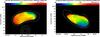 |
Fig. 14 Maps of Faraday rotation measure (color, in rad m-2) of the Sausage relic (left) and the Toothbrush relic (right), computed for regions where the polarized intensity exceeds ten times the rms noise σQU in U and Q at both frequencies. The contours show the polarized intensity at 8.35 GHz at [1, 2, 3, 4, 6] × 0.3 mJy/beam for the Sausage relic (left) and at [1, 2, 3, 4, 6, 8, 10] × 0.5 mJy/beam for the Toothbrush relic (right). The beam sizes are 159″ × 159″. The RM of + 532 ± 39 rad m-2 of source D south of the Sausage relic is beyond the color range and is not shown in the left figure. |
As we observe only at two frequencies, the rotation measure was estimated assuming a linear dependency of the polarization angle χ and the wavelength λ: 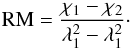 (7)This method gives average Faraday rotation angles, which are not corrected for redshift. Information on the complexity of the relics in Faraday space would need broadband polarimetric data and application of RM Synthesis (Sect. 4).
To obtain the rotation measure maps, we convolved the Stokes U and Q maps at 8.35 GHz to the resolution of the 4.85 GHz maps of 159″. The final RM maps were made using the low-resolution maps of polarization angles, clipped below a signal-to-noise ratio of Sp = PI /σUQ = 10, where σUQ is the rms noise in U and Q at both frequencies (see Tables 2 and 3). The error in RM is  , which is ΔRM ≃ 28 rad m-2 for Sp = 10. The ± nπ ambiguity of polarization angles corresponds to a large RM ambiguity of ± n × 1241 rad m-2 that can be excluded for our data.
The results of the RM analysis are shown in Fig. 14 for the two bright radio relics. No RM maps are shown for the two faint relics because RM can only be measured in a small region for these candidates.
The mean RMs between 4.85 GHz and 8.35 GHz in several regions are summarized in Table 7, computed from the average Stokes U and Q values at both frequencies. The uncertainties in the mean RM were estimated from error propagation, using the rms noise in U and Q at both frequencies.
For the Sausage radio relic in CIZA J2242, we find RMs between −150 rad m-2 and −180 rad m-2. The values are in agreement with the average value of −140 rad m-2 obtained at 1.2–1.8 GHz (van Weeren et al. 2010). If regular fields within the relic generated the large observed values of RM, total depolarization by differential Faraday rotation has to occur at 1.2–1.8 GHz (see e.g. Arshakian & Beck 2011), which is not the case. As the anisotropic magnetic fields in relics do not give rise to Faraday rotation, the RM probably originates in the foreground. Located near to the plane of the Milky Way at Galactic coordinates of l = 104°, b = −5°, strong Faraday rotation is expected. The interactive catalog that is based on Oppermann et al. (2012) gives a mean value of RM = −73 ± 70 rad m-2 around the relic position (Table 7), which is consistent with our result. An RM gradient of about 12 rad m-2 per arcminute along the relic (Fig. 15 left) is indicated, which is much larger than the predictions of the RM foreground by Sun & Reich (2009). A refined run of this simulation towards the Sausage relic at a resolution of 2.5′ gives an RM gradient of only about 10 rad m-2 per degree (Reich, priv. comm.).
Mean RMs between 4.85 GHz and 8.35 GHz and in the Galactic foreground.
Source D in CIZA J2242+53 is a bright head-tail radio galaxy (Stroe et al. 2013) for which we find a very high RM of + 532 ± 39 rad m-2 (Fig. 14 left, bottom) that most probably originates from the radio lobes of the galaxy itself. The average RM of the Toothbrush relic is also consistent with the value of the Galactic foreground (Table 7). An RM gradient of about 15 rad m-2 per arcminute along the relic is indicated. Again, this type of gradient is much larger than the Galactic foreground can produce. RM Synthesis was applied to the data in the 1.38 GHz band by van Weeren et al. (2012). They found an even larger RM difference between components B1 (−53 rad m-2) and B2 (+ 55 rad m-2). Strong Faraday rotation is also obvious when comparing the apparent B–vectors between 1.38 GHz and 4.9 GHz (Fig. 4). No RM map was computed between these frequencies because the small RM ambiguity of ±n × 72 rad m-2 does not enable us to obtain reliable RM values.
For ZwCl and A 1612 no RM values have been published so far. While the small RMs for A 1612 are consistent with its high Galactic latitude of b = + 60°, RM ≃ −60 rad m-2 for ZwCl deviates from the average value estimated from the catalog by Oppermann et al. (2012). For the large radio relic in Abell 2256, a high resolution RM map obtained with JVLA observations in the frequency range from 1 to 8 GHz has been published (Owen et al. 2014). The map shows large coherent RM patches with RM values ranging from about −70 to about −20 rad m-2. The RM gradients are significantly larger than expected for the Galactic foreground.
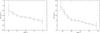 |
Fig. 15 Profile of not foreground subtracted rotation measures of the Sausage relic (left) and the Toothbrush relic (right) in sectors of 1′ width (corresponding to 5° and 2° azimuthal angle along the ring for the Sausage and Toothbrush relics, respectively) and of 3′ thickness in radius. The azimuthal angle on the horizontal axis is measured counter-clockwise from the north-south direction. The ring for each relic is centered at the approximate cluster center and follows the shape of the relic. The error bars are computed from the rms noise of U and Q in each sector. |
The generation of RM and RM gradients needs large-scale regular magnetic fields that preserve their directions over the extent of the relics of several Mpc, much larger than the coherence length of the turbulent (or tangled) field. A large-scale α−Ω dynamo cannot operate in a similar fashion to spiral galaxies because galaxy clusters do not have an organized rotation. The magneto-thermal instability may generate radially ordered fields in the ICM (Pfrommer & Dursi 2010), but without coherent directions. Simulations indicate that the strengths of large-scale intergalactic magnetic fields are about 100 nG around galaxy clusters and about 10 nG in filaments of the cosmic web (e.g. Ryu et al. 2008). With electron densities of typically ⟨ ne ⟩ = 10-4 cm-3 at R500 (Croston et al. 2008), a pathlength through the regular field (coherence length) of 1–10 Mpc is needed to achieve 10 rad m-2. Large-scale filaments with coherent RMs were found in the relic of Abell 2256 (Owen et al. 2014). The observed lengths of several 100 kpc are limited by the extent of synchrotron emission, while the magnetic filaments could be much larger. Recent MHD simulations indicate magnetic filaments on these scales (Vazza, priv. comm.). Our observations give evidence that these types of large-scale intergalactic fields may exist around galaxy clusters.
As a note of caution, we have to admit that the RMs in Fig. 14 are based on measurements of polarization angles in only two relatively narrow frequency bands. If the polarization angle is not proportional to λ2, e.g. due to Faraday depolarization or internal structure of the emitting and Faraday-rotating source (a complex distribution of Faraday rotating and synchrotron emitting media), two-point RMs are not reliable. The first issue can be excluded because Faraday depolarization is low for all relics observed in this work (except for component B1 of the Toothbrush relic). Internal structure within the relic cannot be excluded and indeed is a possible scenario (Bonafede et al. 2014). Polarization observations over a wide range in λ2 and application of RM Synthesis (Brentjens & de Bruyn 2005) are needed to measure the Faraday spectrum that contains information about the emitting region. Furthermore, signatures of the turbulent or tangled field should become visible with measurement with high resolution in Faraday space as a so-called Faraday forest of many components in the Faraday spectrum (Beck et al. 2012).
4. Conclusions and discussion
Single-dish radio telescopes like the Effelsberg 100-m are ideal instruments to confirm relic candidates or search for new cluster relic candidates by detecting their polarization, as long as the map area is sufficient to achieve reliable baselines, to determine meaningful rms noise values and, hence, to measure the total and polarized flux densities with small uncertainties. Although the resolution is limited owing to the large beam size, magnetic fields in cluster relics are highly ordered, so that the degree of polarization only weakly decreases with increasing beam size. Even relics with angular extents smaller than the telescope beam still reveal significant polarization, if the curvature of the shock front is small within the beam.
Galaxy cluster relics are among the most highly polarized sources on sky. In the two prominent Mpc-sized radio relics, the Sausage (in the cluster CIZA J2242+53) and the Toothbrush (1RXS 06+42), we found maximum polarization degrees of about 50% at 8.35 GHz, which are among the highest fractions of linear polarization detected in any extragalactic radio source, indicating strong shocks (high Mach numbers). We also detected polarization from the eastern relic in the cluster ZwCl 0008+52 and from a relic in Abell 1612. The maximum degrees of polarization of the latter two relics are smaller (20–30%) because either their shock strengths are lower and/or the relics are inclined to the sky plane.
The radio spectra below 8.35 GHz can be well fitted by single power laws for all four relics. Possible spectral breaks toward higher frequencies (Stroe et al. 2016) need confirmation by further observations and corrections for the SZ effect (Basu et al. 2016). The flat average spectral indices of 0.9 and 1.0 for the Sausage and the Toothbrush relics indicate that models describing the origin of relics have to include effects beyond the assumptions of diffuse shock acceleration. The steep radio spectra for the relics in ZwCl 0008+52 and Abell 1612 give additional evidence for low Mach numbers of ≈2.4.
The total field strengths of the relics are in the range of 2.4–4.2 μG, assuming equipartition between the energy densities of cosmic rays and a proton-to-electron ratio of 100. These field strengths are in accord with upper limits of the IC emission. It has been proposed that, at merger shocks, electrons are accelerated via shock drift acceleration (Guo et al. 2014a). This process is only possible for a high plasma–β upstream of the shock (β ≳ 20). If only electrons are accelerated the proton-to-electron ratio is 0 and the corresponding estimates of magnetic field strengths become 0.7–1.2 μG, which fulfills the high plasma–β requirement. However, these fields are in tension with the limits derived from IC emission. Deeper IC measurements of the cosmic-ray electron density are required to solve this discrepancy.
We observed Abell 1612 with the Chandra telescope. The complex X-ray surface brightness distribution reveals an ongoing major merger after the first core passage and supports the classification of the diffuse emission as a radio relic.
No wavelength-dependent Faraday depolarization is detected between 4.85 GHz and 8.35 GHz, except for one component of the Toothbrush relic, confirming the low density of thermal electrons within the relic and within the ICM in front of the relic. Faraday depolarization is significant for the Toothbrush relic between 1.38 GHz and 8.35 GHz and varies with distance from the cluster center. This can be explained by a decrease in electron density and strength of the turbulent field. We conclude that measurements of Faraday depolarization at radio frequencies of several GHz, preferably with single-dish telescopes, which trace the full extended emission, enable us to put constraints on the properties of the intracluster medium.
Faraday rotation measures along the relics reveal large-scale gradients that are much larger than those expected in the Milky Way foreground. This gives evidence for large-scale intergalactic fields around the clusters.
Polarization observations with synthesis telescopes at low or moderate frequencies that cover a wide range in λ2 and application of RM Synthesis (Brentjens & de Bruyn 2005) will allow us to measure the Faraday spectrum and extract information on the internal structure of the emitting region and the turbulent medium in the cluster foreground.
In this paper we use “vector” for the orientation of the magnetic plane of the incoming electromagnetic wave.
Acknowledgments
The authors acknowledge support from the DFG Research Unit FOR1254. We thank the referee for helpful comments. We thank Alice di Vicenzo for performing a part of the observations and the operators at the Effelsberg telescope for their support. We thank Dr. Aritra Basu (MPIfR) for supporting us with the interpretation of our data and for valuable suggestions to improve the paper. We thank Wolfgang Reich (MPIfR) and Franco Vazza (Hamburger Sternwarte) for important contributions to the discussion. We thank Felipe Andrade-Santos for providing various Chandra data reduction scripts. R.J.W. is supported by a Clay Fellowship awarded by the Harvard-Smithsonian Center for Astrophysics. W. R. Forman and C. Jones acknowledge support from the Smithsonian Institution and the Chandra HRC GTO Program.
References
- Arshakian, T. G., & Beck, R. 2011, MNRAS, 418, 2336 [NASA ADS] [CrossRef] [Google Scholar]
- Basu, K., Vazza, F., Erler, J., & Sommer, M. 2016, A&A, 591, A142 [NASA ADS] [CrossRef] [EDP Sciences] [Google Scholar]
- Beck, R., & Krause, M. 2005, Astron. Nachr., 326, 414 [NASA ADS] [CrossRef] [Google Scholar]
- Beck, R., Frick, P., Stepanov, R., & Sokoloff, D. 2012, A&A, 543, A113 [NASA ADS] [CrossRef] [EDP Sciences] [Google Scholar]
- Bell, A. R. 1978, MNRAS, 182, 443 [NASA ADS] [CrossRef] [Google Scholar]
- Blandford, R., & Eichler, D. 1987, Phys. Rep., 154, 1 [Google Scholar]
- Bonafede, A., Giovannini, G., Feretti, L., Govoni, F., & Murgia, M. 2009, A&A, 494, 429 [NASA ADS] [CrossRef] [EDP Sciences] [Google Scholar]
- Bonafede, A., Vazza, F., Brüggen, M., et al. 2013, MNRAS, 433, 3208 [NASA ADS] [CrossRef] [Google Scholar]
- Bonafede, A., Intema, H. T., Brüggen, M., et al. 2014, ApJ, 785, 1 [NASA ADS] [CrossRef] [Google Scholar]
- Botteon, A., Gastaldello, F., Brunetti, G., & Dallacasa, D. 2016, MNRAS, 460, L84 [NASA ADS] [CrossRef] [Google Scholar]
- Brentjens, M. A., & de Bruyn, A. G. 2005, A&A, 441, 1217 [NASA ADS] [CrossRef] [EDP Sciences] [Google Scholar]
- Brüggen, M., van Weeren, R. J., & Röttgering, H. J. A. 2012, MNRAS, 425, L76 [NASA ADS] [CrossRef] [Google Scholar]
- Burn, B. J. 1966, MNRAS, 133, 67 [NASA ADS] [CrossRef] [Google Scholar]
- Croston, J. H., Pratt, G. W., Böhringer, H., et al. 2008, A&A, 487, 431 [NASA ADS] [CrossRef] [EDP Sciences] [Google Scholar]
- de Gasperin, F., Intema, H. T., van Weeren, R. J., et al. 2015, MNRAS, 453, 3483 [NASA ADS] [CrossRef] [Google Scholar]
- Donnert, J. M. F., Stroe, A., Brunetti, G., Hoang, D., & Roettgering, H. 2016, MNRAS, 462, 2014 [NASA ADS] [CrossRef] [Google Scholar]
- Emerson, D. T., & Gräve, R. 1988, A&A, 190, 353 [NASA ADS] [Google Scholar]
- Emerson, D. T., Klein, U., & Haslam, C. G. T. 1979, A&A, 76, 92 [NASA ADS] [Google Scholar]
- Enßlin, T. A., & Gopal-Krishna. 2001, A&A, 366, 26 [NASA ADS] [CrossRef] [EDP Sciences] [Google Scholar]
- Enßlin, T. A., Biermann, P. L., Klein, U., & Kohle, S. 1998, A&A, 332, 395 [NASA ADS] [Google Scholar]
- Feretti, L., Giovannini, G., Klein, U., et al. 1998, A&A, 331, 475 [NASA ADS] [Google Scholar]
- Feretti, L., Giovannini, G., Govoni, F., & Murgia, M. 2012, A&ARv, 20, 54 [Google Scholar]
- Finoguenov, A., Sarazin, C. L., Nakazawa, K., Wik, D. R., & Clarke, T. E. 2010, ApJ, 715, 1143 [NASA ADS] [CrossRef] [Google Scholar]
- Govoni, F., & Feretti, L. 2004, Int. J. Mod. Phys. D, 13, 1549 [NASA ADS] [CrossRef] [Google Scholar]
- Govoni, F., Feretti, L., Giovannini, G., et al. 2001, A&A, 376, 803 [NASA ADS] [CrossRef] [EDP Sciences] [Google Scholar]
- Guo, X., Sironi, L., & Narayan, R. 2014a, ApJ, 794, 153 [NASA ADS] [CrossRef] [Google Scholar]
- Guo, X., Sironi, L., & Narayan, R. 2014b, ApJ, 797, 47 [NASA ADS] [CrossRef] [Google Scholar]
- Haslam, C. G. T. 1974, A&AS, 15, 333 [NASA ADS] [Google Scholar]
- Hoeft, M., & Brüggen, M. 2007, MNRAS, 375, 77 [NASA ADS] [CrossRef] [Google Scholar]
- Hoeft, M., Brüggen, M., Yepes, G., Gottlöber, S., & Schwope, A. 2008, MNRAS, 391, 1511 [NASA ADS] [CrossRef] [Google Scholar]
- Hong, S. E., Kang, H., & Ryu, D. 2015, ApJ, 812, 49 [NASA ADS] [CrossRef] [Google Scholar]
- Itahana, M., Takizawa, M., Akamatsu, H., et al. 2015, PASJ, 67, 113 [NASA ADS] [CrossRef] [Google Scholar]
- Kalberla, P. M. W., Burton, W. B., Hartmann, D., et al. 2005, A&A, 440, 775 [NASA ADS] [CrossRef] [EDP Sciences] [Google Scholar]
- Kale, R., Dwarakanath, K. S., Bagchi, J., & Paul, S. 2012, MNRAS, 426, 1204 [NASA ADS] [CrossRef] [Google Scholar]
- Kocevski, D. D., Ebeling, H., Mullis, C. R., & Tully, R. B. 2007, ApJ, 662, 224 [NASA ADS] [CrossRef] [Google Scholar]
- Laing, R. A. 1980, MNRAS, 193, 439 [NASA ADS] [Google Scholar]
- Lindner, R. R., Baker, A. J., Hughes, J. P., et al. 2014, ApJ, 786, 49 [NASA ADS] [CrossRef] [Google Scholar]
- Mack, K. H., Klein, U., Saripalli, L., Willis, A. G., & O’Dea, C. P. 1996, in Extragalactic Radio Sources, eds. R. D. Ekers, C. Fanti, & L. Padrielli, IAU Symp., 175, 317 [Google Scholar]
- Marcowith, A., Bret, A., Bykov, A., et al. 2016, Rep. Prog. Phys., 79, 046901 [NASA ADS] [CrossRef] [Google Scholar]
- Markevitch, M., Govoni, F., Brunetti, G., & Jerius, D. 2005, ApJ, 627, 733 [NASA ADS] [CrossRef] [Google Scholar]
- Murgia, M., Govoni, F., Feretti, L., et al. 2004, A&A, 424, 429 [NASA ADS] [CrossRef] [EDP Sciences] [Google Scholar]
- Murgia, M., Govoni, F., Carretti, E., et al. 2016, MNRAS, 461, 3516 [NASA ADS] [CrossRef] [Google Scholar]
- Ogrean, G. A., Brüggen, M., Röttgering, H., et al. 2013a, MNRAS, 429, 2617 [NASA ADS] [CrossRef] [Google Scholar]
- Ogrean, G. A., Brüggen, M., van Weeren, R. J., et al. 2013b, MNRAS, 433, 812 [NASA ADS] [CrossRef] [Google Scholar]
- Ogrean, G. A., Brüggen, M., van Weeren, R., et al. 2014, MNRAS, 440, 3416 [NASA ADS] [CrossRef] [Google Scholar]
- Oppermann, N., Junklewitz, H., Robbers, G., et al. 2012, A&A, 542, A93 [NASA ADS] [CrossRef] [EDP Sciences] [Google Scholar]
- Owen, F. N., Rudnick, L., Eilek, J., et al. 2014, ApJ, 794, 24 [NASA ADS] [CrossRef] [Google Scholar]
- Peng, B., Kraus, A., Krichbaum, T. P., & Witzel, A. 2000, A&AS, 145, 1 [NASA ADS] [CrossRef] [EDP Sciences] [Google Scholar]
- Perley, R. A., & Butler, B. J. 2013, ApJS, 206, 16 [Google Scholar]
- Pfrommer, C., & Dursi, L. 2010, Nature Phys., 6, 520 [Google Scholar]
- Ryu, D., Kang, H., Cho, J., & Das, S. 2008, Science, 320, 909 [NASA ADS] [CrossRef] [PubMed] [Google Scholar]
- Sarazin, C. L. 1999, ApJ, 520, 529 [NASA ADS] [CrossRef] [Google Scholar]
- Skillman, S. W., Hallman, E. J., O’Shea, B. W., et al. 2011, ApJ, 735, 96 [NASA ADS] [CrossRef] [Google Scholar]
- Slee, O. B., Roy, A. L., Murgia, M., Andernach, H., & Ehle, M. 2001, AJ, 122, 1172 [NASA ADS] [CrossRef] [Google Scholar]
- Sokoloff, D. D., Bykov, A. A., Shukurov, A., et al. 1998, MNRAS, 299, 189 [NASA ADS] [CrossRef] [Google Scholar]
- Stroe, A., van Weeren, R. J., Intema, H. T., et al. 2013, A&A, 555, A110 [NASA ADS] [CrossRef] [EDP Sciences] [Google Scholar]
- Stroe, A., Shimwell, T., Rumsey, C., et al. 2016, MNRAS, 455, 2402 [NASA ADS] [CrossRef] [Google Scholar]
- Sun, X. H., & Reich, W. 2009, A&A, 507, 1087 [NASA ADS] [CrossRef] [EDP Sciences] [Google Scholar]
- van Weeren, R. J., Röttgering, H. J. A., Brüggen, M., & Hoeft, M. 2010, Science, 330, 347 [NASA ADS] [CrossRef] [PubMed] [Google Scholar]
- van Weeren, R. J., Brüggen, M., Röttgering, H. J. A., & Hoeft, M. 2011a, MNRAS, 418, 230 [Google Scholar]
- van Weeren, R. J., Brüggen, M., Röttgering, H. J. A., et al. 2011b, A&A, 533, A35 [NASA ADS] [CrossRef] [EDP Sciences] [Google Scholar]
- van Weeren, R. J., Hoeft, M., Röttgering, H. J. A., et al. 2011c, A&A, 528, A38 [NASA ADS] [CrossRef] [EDP Sciences] [Google Scholar]
- van Weeren, R. J., Röttgering, H. J. A., Intema, H. T., et al. 2012, A&A, 546, A124 [NASA ADS] [CrossRef] [EDP Sciences] [Google Scholar]
- van Weeren, R. J., Brunetti, G., Brüggen, M., et al. 2016, ApJ, 818, 204 [NASA ADS] [CrossRef] [Google Scholar]
- Vazza, F., Brüggen, M., van Weeren, R., et al. 2012, MNRAS, 421, 1868 [NASA ADS] [CrossRef] [Google Scholar]
- Vazza, F., Eckert, D., Brüggen, M., & Huber, B. 2015, MNRAS, 451, 2198 [NASA ADS] [CrossRef] [Google Scholar]
- Vikhlinin, A., Markevitch, M., Murray, S. S., et al. 2005, ApJ, 628, 655 [NASA ADS] [CrossRef] [Google Scholar]
- Voges, W., Aschenbach, B., Boller, T., et al. 1999, A&A, 349, 389 [NASA ADS] [Google Scholar]
- Wardle, J. F. C., & Kronberg, P. P. 1974, ApJ, 194, 249 [NASA ADS] [CrossRef] [Google Scholar]
- Xu, J. W., Han, J. L., Sun, X. H., et al. 2007, A&A, 470, 969 [NASA ADS] [CrossRef] [EDP Sciences] [Google Scholar]
All Tables
Equipartition magnetic field strengths (assuming a proton-to-electron ratio of K = 100).
All Figures
|
Fig. 1 Polarized emission (color) of the Sausage relic in CIZA J2242+53, overlaid with total intensity contours. Vectors depict the polarization B–vectors, not corrected for Faraday rotation, with lengths representing the degree of polarization. Left: 8.35 GHz map. Total intensity contours are drawn at levels of [1, 2, 3, 4, 6, 8, 16] × 1.2 mJy/beam. A vector length of 1′ corresponds to 90% fractional polarization. The beam size is 90″ × 90″. The sources are labeled according to Stroe et al. (2013). Right: 4.85 GHz map. Total intensity contours are drawn at levels of [1, 2, 3, 4, 6, 8, 16] × 2.4 mJy/beam. A vector length of 1′ corresponds to 50% fractional polarization. The beam size is 159″ × 159″. |
| In the text | |
|
Fig. 2 Polarized emission (color) of the Toothbrush relic in 1RXS 06+42, overlaid with total intensity contours. Vectors depict the polarization B–vectors, not corrected for Faraday rotation, with lengths representing the degree of polarization. Left: 8.35 GHz map. Total intensity contours are drawn at levels of [1, 2, 3, 4, 6, 8, 16] × 1.5 mJy/beam. A vector length of 1′ corresponds to 90% fractional polarization. The beam size is 90″ × 90″. The sources are labeled according to van Weeren et al. (2012). Right: 4.85 GHz map. Total intensity contours are drawn at levels of [1, 2, 3, 4, 6, 8, 16] × 3 mJy/beam. A vector length of 1′ corresponds to 30% fractional polarization. The beam size is 159″ × 159″. |
| In the text | |
|
Fig. 3 Polarized emission (color) of the Toothbrush relic 1RXS 06+42 at 8.35 GHz in Stokes U (left) and Stokes Q (right), overlaid with total intensity contours. Vectors depict the polarization B–vectors, not corrected for Faraday rotation, with lengths representing the polarized intensity. (1′ ≡ 3 mJy/beam). Total intensity contours are drawn at levels of [1, 2, 3, 4, 6, 8, 16] × 1.5 mJy/beam. The beam size is 90″ × 90″. |
| In the text | |
|
Fig. 4 Polarized emission (color) of the Toothbrush relic in 1RXS 06+42, overlaid with total intensity contours, from observations at the Westerbork Radio Synthesis Telescope (WSRT) (van Weeren et al. 2012). Vectors depict the polarization B–vectors, not corrected for Faraday rotation, with lengths representing the degree of polarization. The beam size is 22″ × 34″. Left: 1.38 GHz map. Total intensity contours are drawn at levels of [1, 2, 4, 6, 8, 16, 32] × 1 mJy/beam. A vector length of 1′ corresponds to 20% fractional polarization. Right: 4.9 GHz map. Total intensity contours are drawn at levels of [1, 2, 4, 6, 8, 16, 32] × 1 mJy/beam. A vector length of 1′ corresponds to 75% fractional polarization. The rms noise increases with increasing distance from the center of the primary beam which is obvious at the eastern edge of the map. |
| In the text | |
|
Fig. 5 Polarized emission (color) of the radio relic in ZwCl 0008+52, overlaid with total intensity contours. Vectors depict the polarization B–vectors, not corrected for Faraday rotation, with lengths representing the degree of polarization. The sources are labeled according to van Weeren et al. (2011c). Left: 8.35 GHz map. Total intensity contours are drawn at levels of [1, 2, 3, 4, 6, 8, 16] × 0.6 mJy/beam. A vector length of 1′ corresponds to 50% fractional polarization. The beam size is 90″ × 90″. Right: 4.85 GHz map. Total intensity contours are drawn at levels of [1, 2, 3, 4, 6, 8, 16] × 2.25 mJy/beam. A vector length of 1′ corresponds to 30% fractional polarization. The beam size is 159″ × 159″. – Note that the map area of the 8.35 GHz measurement (left panel) only includes a small region around the eastern relic (white box in the right panel), whereas the map of the 4.85 GHz measurement (right panel) encompasses the entire cluster. |
| In the text | |
|
Fig. 6 Polarized emission (color) of the radio relic in Abell 1612, overlaid with total intensity contours. Vectors depict the polarization B–vectors, not corrected for Faraday rotation, with lengths representing the degree of polarization. Left: 8.35 GHz map. Total intensity contours are drawn at levels of [1, 2, 3, 4, 6, 8, 16] × 1.5 mJy/beam. A vector length of 1′ corresponds to 30% fractional polarization. The beam size is 90″ × 90″. Right: 4.85 GHz map. Total intensity contours are drawn at levels of [1, 2, 3, 4, 6, 8, 16] × 1.5 mJy/beam. A vector length of 1′ corresponds to 20% fractional polarization. The beam size is 159″ × 159″. |
| In the text | |
|
Fig. 7 X-ray emission (color) of Abell 1612 taken with Chandra and smoothed to a beam size of 30″ × 30″, overlaid with contours of total radio emission at 8.35 GHz with a beam size of 90″ × 90″. Contours are drawn at levels of [1, 2, 3, 4, 6, 8, 16] × 1.5 mJy/beam. |
| In the text | |
|
Fig. 8 Overlay of a WHT image of Abell 1612 with the X-ray surface brightness (red-yellow contours) and the total radio emission at 8.35 GHz (blue contours). |
| In the text | |
|
Fig. 9 Integrated total intensity spectra of the relics considered in this paper. Top left: spectrum of the Sausage radio relic. The flux densities at frequencies lower than 4.85 GHz are taken from Table 3 of Stroe et al. (2016). Top right: spectrum of the Toothbrush radio relic. The flux densities at frequencies lower than 4.85 GHz are taken from Table 3 of Stroe et al. (2016). Bottom left: spectrum of the radio relic in ZwCl 0008+52. The flux densities at frequencies lower than 4.85 GHz are taken from van Weeren et al. (2011c). Bottom right: spectrum of the radio relic in Abell 1612. The flux densities at frequencies lower than 4.85 GHz are taken from van Weeren et al. (2011b). |
| In the text | |
|
Fig. 10 Sketch for the path length through the emitting volume of a relic. The width of the downstream volume is given by the cooling time of the electrons. The green line indicates the line of sight with the maximum path length through the emitting volume. d is the intrinsic width and ΔR the observable width of the relic (see Table 1). For d ≪ Rcc the maximum path length can be approximated by |
| In the text | |
|
Fig. 11 Degree of polarization (color) of the Sausage relic (left) and the Toothbrush relic (right) at 8.35 GHz with 90″ × 90″ resolution. The contours show the polarized intensity at [1, 2, 4, 6] × 0.21 mJy/beam for the Sausage relic (left) and at [1, 2, 4, 6, 8] × 0.39 mJy/beam for the Toothbrush relic (right). |
| In the text | |
|
Fig. 12 Degree of polarization as a function of the Mach number of the shock. The polarization is derived assuming a weak upstream magnetic field that is isotropically tangled on small scales and compressed at the shock front (Hoeft et al., in prep.). |
| In the text | |
|
Fig. 13 Depolarization between 1.38 GHz and 8.35 GHz (color), defined as DP = p1.38/p8.35, of the Toothbrush relic with a beam size 90″ × 90″, overlaid with contours of polarized intensity at 8.35 GHz. Contours are drawn at levels of [1, 2, 4, 6, 8] × 0.39 mJy/beam. |
| In the text | |
|
Fig. 14 Maps of Faraday rotation measure (color, in rad m-2) of the Sausage relic (left) and the Toothbrush relic (right), computed for regions where the polarized intensity exceeds ten times the rms noise σQU in U and Q at both frequencies. The contours show the polarized intensity at 8.35 GHz at [1, 2, 3, 4, 6] × 0.3 mJy/beam for the Sausage relic (left) and at [1, 2, 3, 4, 6, 8, 10] × 0.5 mJy/beam for the Toothbrush relic (right). The beam sizes are 159″ × 159″. The RM of + 532 ± 39 rad m-2 of source D south of the Sausage relic is beyond the color range and is not shown in the left figure. |
| In the text | |
|
Fig. 15 Profile of not foreground subtracted rotation measures of the Sausage relic (left) and the Toothbrush relic (right) in sectors of 1′ width (corresponding to 5° and 2° azimuthal angle along the ring for the Sausage and Toothbrush relics, respectively) and of 3′ thickness in radius. The azimuthal angle on the horizontal axis is measured counter-clockwise from the north-south direction. The ring for each relic is centered at the approximate cluster center and follows the shape of the relic. The error bars are computed from the rms noise of U and Q in each sector. |
| In the text | |
Current usage metrics show cumulative count of Article Views (full-text article views including HTML views, PDF and ePub downloads, according to the available data) and Abstracts Views on Vision4Press platform.
Data correspond to usage on the plateform after 2015. The current usage metrics is available 48-96 hours after online publication and is updated daily on week days.
Initial download of the metrics may take a while.