| Issue |
A&A
Volume 592, August 2016
|
|
|---|---|---|
| Article Number | A49 | |
| Number of page(s) | 14 | |
| Section | Interstellar and circumstellar matter | |
| DOI | https://doi.org/10.1051/0004-6361/201628550 | |
| Published online | 22 July 2016 | |
Measuring turbulence in TW Hydrae with ALMA: methods and limitations⋆
1 Max-Planck-Institut für Astronomie, Königstuhl 17 69117 Heidelberg Germany
e-mail: teague@mpia.de
2 Univ. Bordeaux, LAB, UMR 5804, 33270 Floirac, France
3 CNRS, LAB, UMR 5804, 33270 Floirac, France
4 IRAM, 300 rue de la Piscine, Domaine Universitaire, 38406 Saint-Martin-d’ Hères, France
5 SETI Institute, 189 Bernardo Avenue, Mountain View, CA 94043, USA
6 NASA Ames Research Center, Moffett Field, CA 94035, USA
Received: 18 March 2016
Accepted: 30 May 2016
Aims. We aim to obtain a spatially resolved measurement of velocity dispersions in the disk of TW Hya.
Methods. We obtained images with high spatial and spectral resolution of the CO J = 2–1, CN N = 2–1 and CS J = 5–4 emission with ALMA in Cycle 2. The radial distribution of the turbulent broadening was derived with two direct methods and one modelling approach. The first method requires a single transition and derives Tex directly from the line profile, yielding a vturb. The second method assumes that two different molecules are co-spatial, which allows using their relative line widths for calculating Tkin and vturb. Finally we fitted a parametric disk model in which the physical properties of the disk are described by power laws, to compare our direct methods with previous values.
Results. The two direct methods were limited to the outer r > 40 au disk because of beam smear. The direct method found vturb to range from ≈130 m s-1 at 40 au, and to drop to ≈50 m s-1 in the outer disk, which is qualitatively recovered with the parametric model fitting. This corresponds to roughly 0.2−0.4 cs. CN was found to exhibit strong non-local thermal equilibrium effects outside r ≈ 140 au, so that vturb was limited to within this radius. The assumption that CN and CS are co-spatial is consistent with observed line widths only within r ≲ 100 au, within which vturb was found to drop from 100 m s-1 (≈0.4 cs) to zero at 100 au. The parametric model yielded a nearly constant 50 m s-1 for CS (0.2−0.4 cs). We demonstrate that absolute flux calibration is and will be the limiting factor in all studies of turbulence using a single molecule.
Conclusions. The magnitude of the dispersion is comparable with or below that predicted by the magneto-rotational instability theory. A more precise comparison would require reaching an absolute calibration precision of about 3%, or finding a suitable combination of light and heavy molecules that are co-located in the disk.
Key words: techniques: interferometric / turbulence / methods: observational / ISM: kinematics and dynamics / submillimeter: ISM
The reduced datacubes (FITS files) are only available at the CDS via anonymous ftp to cdsarc.u-strasbg.fr (130.79.128.5) or via http://cdsarc.u-strasbg.fr/viz-bin/qcat?J/A+A/592/A49
© ESO, 2016
1. Introduction
Turbulent motions underpin the entire evolution of a protoplanetary disk. Foremost, turbulence determines the bulk gas viscosity and hence regulates the angular momentum transport and accretion in disks (Shakura & Sunyaev 1973; Pringle 1981). Secondly, turbulence is a key factor for dust evolution and transport in disks (Testi et al. 2014; Henning & Meeus 2011). However, until recently, observational constraints on the level of disk turbulence were extremely challenging to obtain and hence scarce. With the advent of the Atacama Large Millimeter/submillimeter Array (ALMA), we have access for the first time to observations with the high sensitivity and spectral and angular resolution that are needed to directly measure turbulent velocities in disks.
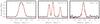 |
Fig. 1 Example spectra of CO (left), CN (centre) and CS (right). All spectra are from a pixel removed by 1″ from the centre. This example only shows three hyperfine components for CN. The red lines show example fits to the data, CO being an optically broadened Gaussian, CN the ensemble of Gaussians, one for each hyperfine component, and CS a pure, optically thin Gaussian. Note that the spectra are Nyquist sampled in velocity. |
Accurate determination of the turbulent velocity dispersion from line broadening requires a good understanding of the other components that contribute to the line width, namely bulk motions of the gas, thermal broadening and, in the case of a highly optically thick line, broadening due to the line opacity. All previous measurements of vturb have revolved around the fitting of a parametric model to extract a disk-averaged turbulent broadening value. The derived values ranged from very low values of ≲10–100 m s-1 (≲0.02–0.2 cs) derived for the TW Hya and HD 163296 disks, to higher velocities of ≲100–200 m s-1 (≲0.3–0.5 cs) for the disks of DM Tau, MWC 480 and LkCa 15 (Dartois et al. 2003; Piétu et al. 2007; Hughes et al. 2011; Rosenfeld et al. 2012; Flaherty et al. 2015). With the exception of TW Hya and HD 163296 (Hughes et al. 2011; Flaherty et al. 2015), the spectral resolution of the data used to determine these values, of the order ~200 m s-1, is too coarse to resolve the small expected contribution from turbulent broadening, although Guilloteau et al. (2012) did correct for this effect when using CS to measure turbulence in DM Tau.
High-quality ALMA Cycle 2 observations of TW Hya allow us for the first time to obtain a direct measure of the line widths and thus of the spatially resolved turbulent velocity structure. With a nearly face-on inclination of only i ≈ 7° (Qi et al. 2004) and as the nearest protoplanetary disk at d ≈ 54 pc, TW Hya provides the best opportunity to directly detect turbulent broadening as the effect of Keplerian shear for such face-on disks is minimized compared to more inclined systems.
We present here the first direct measurements of vturb in a protoplanetary disk using the line emission of CO, CN and CS. In Sect. 2 we describe our ALMA observations and the data reduction. Section 3 describes the methods we used to extract vturb: two direct methods relying on a measure of the line widths and a more commonly used fit of a parametric model. Discussion in Sect. 4 follows.
2. Observations
The observations were performed using ALMA on May 13, 2015 under excellent weather conditions (Cycle 2, 2013.1.00387.S). The receivers were tuned to cover CO J = (2−1), CS J = (5−4) and all strong hyperfine components of CN N = (2−1) simultaneously. The correlator was configured to deliver very high spectral resolution, with a channel spacing of 15 kHz (and an effective velocity resolution of 40 m s-1) for the CO J = (2−1) and CS J = (5−4) lines, and 30 kHz (80 m s-1) for the CN N = (2−1) transition.
Data were calibrated using the standard ALMA calibration script in the CASA software package1. The calibrated data were regridded in velocity to the LSR frame, and exported through UVFITS format to the GILDAS2 package for imaging and data analysis. Self-calibration was performed on the continuum data, and the phase solution was applied to all spectral line data. With robust weighting, the uv coverage, which has baselines between 21 and 550 m provided by the ~34 antennas, yields a beam size of 0.50″ × 0.42″ at a position angle of 80°. The absolute flux calibration was made with reference to Ganymede. The derived flux for our amplitude and phase calibrator, J1037-2934, was 0.72 Jy at 228 GHz at the time of the observations, with a spectral index α = −0.54, while the ALMA flux archive indicated a flux of 0.72 ± 0.05 Jy between April 14 and April 25. We hence estimate that the calibration uncertainty is about 7%.
After deconvolution and primary beam correction, the data cubes were imported into CLASS for further analysis, in particular line profile fits including the hyperfine structure for CN lines. For the azimuthal average, each spectrum was shifted in velocity from its local projected Keplerian velocity before averaging. We used for this the best-fit Keplerian model assuming a stellar mass of 0.69 M⊙ and i = 7°, see Sect. 3.5.
All three emission lines show azimuthal symmetry within the noise justifying our choice to azimuthally average the data. CO emission looks identical to previous studies (for example Qi et al. 2013), while integrated intensity plots for CN, including all hyperfine components, and CS are shown in Appendix C. Sample spectra illustrating the very high signal-to-noise ratio obtained in CO and CN and the noisier CS data, are given in Fig. 1 and a gallery of azimuthally averaged spectra at different radial locations can be found in Appendix C. Finally, examples of the full complement of CN hyperfine components are shown in Fig. C.3.
3. Separating turbulent velocity dispersions
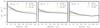 |
Fig. 2 Measured line widths (black) and those corrected for the Keplerian shear component (blue) for CO (left), CN (centre) and CS (right). All three lines are subject to the same Keplerian shear component. The uncertainties include an uncertainty on the inclination of the disk of ±2° as described in Eq. (2). The solid yellow lines show the line widths from the global fit. |
Turbulent motions within a gas manifest themselves as a velocity dispersion along the line of sight, broadening the width of the emission (or absorption) line. This broadening term acts in tandem with thermal broadening, a contribution typically an order of magnitude larger than the turbulent width. Additionally, the Keplerian shear across the beam will broaden the observed emission lines. This effect is the most dominant in the inner disk and for highly inclined disks, making TW Hya an ideal source as this effect is minimized.
In the following section we discuss three methods to for extracting vturb, the turbulent velocity dispersion: two direct ways and one parametric approach, and apply each to TW Hya.
3.1. Line width measurements
Physical parameters were extracted from the line profiles at each pixel in the image and for an azimuthal average. CO is highly optically thick and displays a saturated core meaning the line profile deviates strongly from an optically thin Gaussian (see left panel of Fig. 1). By fitting a line profile of the form ![\begin{equation} I_v = \Big(J_{\nu}(T_{\rm ex}) - J_{\nu}(T_{\rm bg}) \Big) \cdot \left( 1 - \exp \left[-\tau \exp \left\{ -\frac{(v - v_0)^2}{\Delta V^2}\right\} \right] \right), \end{equation}](/articles/aa/full_html/2016/08/aa28550-16/aa28550-16-eq32.png) (1)where Tbg = 2.75 K, we are able to obtain the line full-width at half maximum, FWHM, line centre v0, and if the line is sufficiently optically thick, Tex and τ (otherwise only the product is constrained).
(1)where Tbg = 2.75 K, we are able to obtain the line full-width at half maximum, FWHM, line centre v0, and if the line is sufficiently optically thick, Tex and τ (otherwise only the product is constrained).
Under the assumption that all hyperfine components arise from the same region in the disk and that the main component is optically thick, the relative intensities of the CN hyperfine components yield an optical depth and Tex. Using the hyperfine mode in CLASS, the hyperfine components were simultaneously fit with Gaussian profiles. It was found that the recommended spacing of hyperfine components was systematically biased across the disk, suggesting that the recommended offset values were incorrect. Fitting for the relative positions of each component allowed for a better determination of their spacing to ≈1 m s-1. The adopted frequencies are given in Table A.1.
Finally, the CS emission was well fit by an optically thin Gaussian, from which we were able to accurately extract the line width and line centre. However, with only a single transition the degeneracy between Tex and τ could not be broken so that we remain ignorant of the local temperature.
The line widths are sufficiently well sampled with spectral resolutions of 40 m s-1 for CO and CN and 37 m s-1 for CS such that sampling effects are negligible for our data. Assuming square channels and Gaussian line profiles, we estimate that the bias on the measured ΔV would be ≈2% for CO and CN and ≈3.5% for CS. Figure B.1 shows the effect of the resolution on the determination of ΔV. These biases are included in the following analysis.
3.2. Keplerian shear correction
In the following direct methods we only consider the disk outside 40 au. Within this radius the spectra start to strongly deviate from the assumed Gaussian (in opacity) line profiles, because parts of the disk rotating in opposite directions are smeared in the beam. Given the flux calibration, there is an intrinsic 7% uncertainty on the peak values of the spectra, thus the Tex values derived for CO and CN have uncertainties of at least 7%. The effect of this is discussed in Sect. 4.
To estimate the effect of the artificial broadening that is due to the beam smear, the physical model of TW Hya from Gorti et al. (2011) was used. The model was run through the LIME radiative transfer code (Brinch & Hogerheijde 2010) for a range of inclinations, i = { 0°, 5° ,6° ,7° ,8° ,9° }, assuming no turbulent broadening. We note that the projected velocity is a product of both stellar mass and inclination. By varying only the inclination, we are therefore able to consider uncertainties in both quantities3.
Following Rosenfeld et al. (2013), we accounted for the height above the midplane in the calculation of the velocity field. Both CO J = (2−1) and C18O (2–1) lines were modelled, allowing us to sample an optically thick and thin case. Using CASA, the model observations were converted into synthetic observations with the same array configuration as the true observations. Differences in the resulting line width at each pixel between an inclined disk and a face-on disk were attributed to Keplerian broadening.
At our linear resolution (~25 au), the radial distribution of differences in line widths was well fit by a power law outside of 40 au, 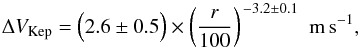 (2)with r the radial distance in au. Quoted uncertainties are 1σ and are dominated by an uncertainty in inclination of ±2°. The differences between the 12CO and C18O cases were smaller than these quoted uncertainties.
This component was subtracted from all line widths prior to further analysis. Figure 2 shows the measured line widths (black lines) and the line widths after the correction for Keplerian shear (blue lines).
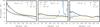 |
Fig. 3 Radial profile of the derived T values (in blue) used for calculating the thermal broadening component of the line width for CO (left), CN (centre) and CS and CN assuming co-spatiality (right). For CO and CN this is Tex while for CS this is Tkin. The black line shows the upper limit Tkin that would fully account for the total line width in the absence of turbulent broadening. Outside 140 au, the derived Tkin exceeds |
3.3. Single molecule approach
After correcting for the Keplerian shear, we assumed that the line width is only a combination of thermal and turbulent broadening. Hence the remaining line width can be described as  (3)where μ is the molecular mass of the tracer molecule, mH the mass of a hydrogen atom, the kinetic temperature of the molecule Tkin, and the line width ΔV = FWHM/
 .
.
For both CO and CN, the line profiles provided Tex, therefore a conversion to Tkin must be made. Guided by the particle densities in the model of Gorti et al. (2011) in the region of expected emission for CO and CN, ≳106–107 cm-3, we assumed that the CO and CN lines are both thermalised so that Tex = Tkin= T. The validity of this assumption is discussed in Sect. 4. The derived Tkin values for CO and CN are shown by the blue lines in the left two panels of Fig. 3. The black lines show  , the highest kinetic temperature in the absence of any turbulence:
 (4)In essence, the residual between these two lines must be accounted for either by turbulent broadening, or sub-thermal excitation, that is, Tkin>T.
Outside of r ~ 140 au, CN shows signs of non-local thermal equilibrium (non-LTE) effects as the derived Tex is considerably higher than  , indicating weak pumping of the line (see Fig. 3). These “supra-thermal” regions are neglected in the remainder of the analysis. The (weak) effect of unresolved turbulence and or temperature gradients on the finite beam size is discussed in Sect. 4.
With a known Tkin a simple subtraction of the thermal broadening component leaves vturb. The left two columns of Fig. 5 show the derived vturb in units of m s-1 in the top panel and as a function of local soundspeed cs in the bottom panel for CO and CN, respectively. Figure 6 shows the spatial distribution of vturb (we here neglected the primary beam correction, which only reaches 7% at the map edge). For CS the line is essentially optically thin, and we cannot derive an excitation temperature.
3.4. Co-spatial approach
Instead of relying on the temperature derived from a single molecule, we can take advantage of molecules with different molecular weights to separate the thermal and turbulent broadening, assuming the lines from these molecules emit from the same location in the disk. Under this assumption the total line widths would be tracing the same vturb and Tkin. Solving Eq. (3) simultaneously for two molecules, A and B with respective molecular masses, μA and μB where μA<μB, and total line widths, ΔVA and ΔVB, we find  This method does not make any assumption about the excitation temperature of the observed transitions, but relies only on the measured line widths and the co-spatiality of the emitting regions.
Of the observed molecules, CO may only trace a narrow layer because of its high optical depth. However, we would expect the optically thin CN and CS to trace a larger vertical region. Both CN and CS would freeze-out at a similar temperature so that the bottom of their respective molecular layers would be relatively coincident and thus might potentially trace the same region in the disk. Hence we chose to apply this method to the two lines of CN and CS.
The rightmost panel of Fig. 3 shows the Tkin (blue line) derived from CN and CS, in comparison to , the maximum Tkin derived from the CS line width (black). Radial profiles of vturb derived from CN and CS are shown in the right column of Fig. 5, in m s-1 (top) and as a function of cs (bottom).
Gaps in Tkin and vturb correspond to the location where the μ-scaled line width of CS is smaller than the μ-scaled line width of CN (see Fig. 7). In this situation there is no solution to Eqs. (5) and (6), thus the assumption of CN and CS being cospatial fails.
3.5. Parametric model fitting
Results of the parametric model fitting.
The above direct methods require a proper correction of the Keplerian shear, which scales as  . For edge-on disks, or when the angular resolution is insufficient to remove the Keplerian shear, our direct technique is not applicable, and the only available method is to use a parametric model assuming Tkin and the total local line width ΔV. A parametric model fit can recover ΔV with high accuracy independently of the absolute (flux) calibration error. However, the fraction of this width that is due to turbulence depends on the absolute calibration since the thermal line width scales as the square root of the kinetic temperature.
In the following we briefly describe of the parametric model but refer to Dartois et al. (2003) and Piétu et al. (2007) for a thorough model description and fitting methodology. The model assumes a disk physical structure that is described by an ensemble of power laws:  (7)for some physical parameter A and cylindrical distance r in au. A positive ea means the A parameter decrease with radius. The molecule densities follow a Gaussian distribution in z, whose scale height H is used as a free parameter (this is equivalent to a uniform abundance in a vertically isothermal disk). This method allows correcting to first order the geometric effects in the projected rotation velocities that are due to disk thickness. CO was found to sample a much higher layer (larger H) than CN or CS which yielded similar values. With this method we fitted two models, firstly one used previously in the literature where vturb is described as a radial power-law, and secondly a model where we fitted for the total line width, ΔV, and then calculated the value of vturb from Eq. (3). We note that fitting for ΔV results in a non-power-law description of vturb.
An inclination, position angle and systemic velocity were found that were comparable to literature values: i ≈ 6°, PA ≈ 240° and VLSR ≈ 2.82 km s-1. Physical parameters relevant to vturb are listed in Table 1 along with their formal errors. All three molecules yielded a steeper dependance of ev than a Keplerian profile with ev ≈ 0.53. This change in projected velocity might either be a projection effect, such as a warp in the disk (Roberge et al. 2005; Rosenfeld et al. 2012), or gas pressure resulting in non-Keplerian rotational velocities for the gas (Rosenfeld et al. 2013). To account for such an exponent with a warp, i needs to change by ≈1° between 40 and 180 au. Thus, while this non-Keplerian bulk motion was not considered explicitly in the removal of the Keplerian shear, the range of inclinations considered, 7 ± 2°, sufficiently account for such a deviation. A more detailed analysis of this is beyond the scope of this paper.
As with the two direct methods, it was assumed that all lines were fully thermalised so that the excitation temperature recovered the full thermal width of the line. A comparison of the total line widths, temperature profiles and turbulent components are shown as yellow solid lines in Figs. 2, 3, and 5, respectively.
4. Results and discussion
In the previous section we have described the three approaches we used to measured vturb in TW Hya. In the following section we compare the methods and discuss their limitations with a view to improving them.
4.1. Temperature structure
Thermal and turbulent broadening are very degenerate, and a precise determination of the temperature structure is therefore a pre-requisite for deriving the level of turbulent broadening. Direct and parametric methods both yield comparable temperatures for CO and CN, as shown in Fig. 3, but we found very different values for vturb, which demonstrates the sensitivity of vturb to the assumed temperature structure.
Excitation temperatures derived from the parametric modelling approach yielded warmer temperatures for CO than for CN, and in turn warmer than CS with T100 = 35.4 ± 0.2 K, 25.3 ± 0.2 K, and 12.2 ± 0.1 K respectively, when fitting for a total line width (see Table 1). This trend was was also seen in the direct methods. These values suggest that the emission from each molecule arises from a different height above the midplane in the disk and therefore could be used to trace the vertical structure of vturb.
In the single-molecule analyis, either direct or parametric, it was assumed that Tex = Tkin for both CO and CN, that is, we assumed that they are both in local thermal equilibrium (LTE). This assumption was guided by the model of Gorti et al. (2011), which has particle densities of ≳106−107 cm-3 from which we assume the molecular emission of CO and CN to arise. This is sufficient to thermalise the CO line. Given that Tkin≥Tex, except from the extremely rare case of supra-thermal excitation, this analysis yielded a lower limit to Tkin, therefore an upper limit to vturb. However, for CN, we have clear evidence for supra-thermal excitation beyond 130 au. A detailed discussion of this issue is beyond the scope of this article. In the future, it will be possible with multiple transitions to use the relative intensities of the transitions to guide modelling of the excitation conditions traced by the molecule, thereby yielding a more accurate scaling of Tex to Tkin.
The co-spatial assumption for CN and CS clearly fails in certain regions of the disk where there is no solution to Eqs. (5) and (6). The temperatures derived from the parametric modelling yield considerably different temperatures for CN and CS (see Table 1), suggesting that this co-spatial assumption fails across the entire disk. Chemical models suggest that CN is present mostly in the photon-dominated layer, higher above the disk plane than CS (although S-bearing molecules are poorly predicted by chemical models, see Dutrey et al. 2011). The non-thermalisation of the CN N = 2−1 line that we observe beyond 130 au also supports the presence of CN relatively high above the disk plane. The accuracy of this assumption can be tested, as well as searching for other co-spatial molecular tracers, with the observation of edge-on disks where the molecular layers can be spatially resolved.
Measurements of temperature will be sensitive to temperature gradients along the line of sight, both vertically and radially. Radial gradients will prove more of a problem than vertical gradients because molecular emission will arise predominantly from a relatively thin vertical region, therefore we expect only a weakly vertical dispersion in temperature. With the temperature profiles discussed in Sect. 3.5, we estimate that the radial average dispersion across the beam is δTbeam ≲ 5% outside 40 au for all three lines with a maximum of ~10% for the very inner regions.
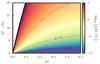 |
Fig. 4 Effect of a temperature dispersion on the accuracy of the measurement of ℳ. The colouring shows how well an input ℳ value can be recovered from a line profile that is the summation of lines at differing temperatures described by δT. |
To understand the effect of this on the subsequent derivation of vturb, we considered a two-zone model. We took two regions with different temperatures but the same turbulent velocity described by a Mach number, ℳtrue = vturb/ and the same optical depth. We measured the temperature and line width using a Gaussian line profile of the resulting combined line profile and derived a Mach number, ℳobs. With this method we are able to explore how accurately ℳobs can recover ℳtrue with a given temperature dispersion. Figure 4 shows the relative error on ℳ, δℳ, as a funtion of ℳtrue and temperature dispersion δT, assuming that the main temperature is 30 K. Taking the temperature dispersions across the beam of 10%, we find an uncertainty of ≲1% for ℳ. This suggests that our determination of vturb is not biased by the expected line-of-sight gradients in temperature and turbulent width.
4.2. Turbulent velocity dispersions
With an assumed thermal structure, the turbulent broadening component was considered to be the residual linewidth that is not accounted for by thermal broadening or beam smear. Resulting values of vturb are compared in Figs. 5 and 6. All three methods yielded values of vturb that ranged from ~50–150 m s-1 corresponding to the range ~0.2–0.4 cs, but they exhibit different radial profiles. The azimuthal structure seen near the centre of the disk in all panels of Fig. 6 is due to the azimuthal-independent subtraction of beam smearing used in Sect. 3.1.
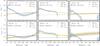 |
Fig. 5 Radial profiles of the turbulent width in m s-1, top row, and as a function of local sound speed, bottom row. The blue dots show the results of the direct method, where the CO and CN lines were assumed to be fully thermalised, and CS to be co-spatial with CN to derive a Tkin value. Yellow solid lines show the results from the global fit where the total line width was fit for, while dashed grey lines show the global fit where vturb was fit for individually. The 1σ uncertainties are shown as bars for the direct method and as shaded regions for the lines. A representative error associated with the flux calibration of 7% at 80 au is shown in the top left corner of all panels. |
4.2.1. Single-molecule approach
CO and CN emission allowed for a single-molecule approach as described in Sect. 3.3. CO yielded values of vturb for 40 ≲ r ≲ 190 au while CN was limited to 40 <r ≲ 130 au because of the potential non-LTE effects described in the previous section. Both molecules displayed a decreasing vturb with radius, although CO has a slight increase in the other edges. As a fraction of cs, both molecules ranged within ~0.2−0.4 cs, but for CO this was found to increase with radius while CN decreased.
4.2.2. Co-spatial approach
Assuming CN and CS are co-spatial, we find vturb values ranging from vturb≤ 100 m s-1 or vturb≤ 0.4 cs, comparable to the range found for CO and CN individually.
This method, however, is limited by the validity that CN and CS are co-spatial. The assumption fails absolutely between 100 ≲ r ≲ 180 au where the linewidth measurements do not allow for a solution of Eqs. (5) and (6) to be found. This is more clearly seen in Fig. 7 which shows the line widths of CN and CS scaled by  where μ = 26 for CN and μ = 44 for CS. In the region where no solution is found, the scaled line width for CS is smaller than that of CN. Despite failing for this molecular pair, this method provides an alternative method to derive Tkin and vturb in another source with a different pair of molecules.
4.2.3. Parametric model fitting
All previous measurements of vturb have relied on fitting a power law model of a disk to the observations (Dartois et al. 2003; Piétu et al. 2007; Hughes et al. 2011; Guilloteau et al. 2012; Rosenfeld et al. 2012; Flaherty et al. 2015), so that allows for a direct comparison to previous results in the literature. In addition, data with reduced spatial and spectral resolution cannot be analysed by the direct methods, therefore it is important to validate the parametric modelling approach.
We have described two models that were fit to the data with the results shown in Table 1. Both include the excitation temperature as a radial power law, but for one we assumed that the total line width is a power law, while for the other we assumed that vturb is a power law. Accordingly, the parameter not fit for is not a power law, but is instead derived through Eq. (3). With high spectral and spatial resolution, the data typically only allow for the this parametric method. A comparison between the models is shown in Fig. 5, where the yellow solid line shows the case where ΔV, the total line width, was assumed to be a power law, and the dashed grey lines show where vturb was assumed to be a power law. All three molecules display similar ranges of vturb, ~50−150 m s-1 (~0.1−0.4 cs) to the direct methods.
For CO and CS the two parametric models yield similar results, but the second, where vturb is fit for, has larger uncertainties. Both molecules have a slightly increasing vturb with radius evturb ≈ −0.22 and − 0.1, respectively, around 60 m s-1. CN, on the other hand, shows a distinct dichotomy between the two that is due to the different temperature profiles derived for the two methods (see Table 1). As mentioned in the previous section, CN displays non-LTE effects that the LTE parametric model may struggle to fit.
A limiting feature of this parametric model fitting is showcased by the results of CO (left column of Fig. 5). If the physical properties of the disk vary from a power-law description, the model will fail to fit this and may be driven to the best average description. For example, while the power-law method recovers vturb for CO for r ≳ 100 au, inside of this radius the two derived vturb values, one directly and one from model fitting, can deviate by up to a factor of 2.
4.3. Limits on the detectability of vturb
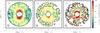 |
Fig. 6 2D distribution of vturb for all three lines: CO (left), CN (centre), and the combination of CN and CS assuming co-spatiality, therefore sharing the same Tex and vturb values (right). The values are masked outside 180 au and within 40 au. The beam size is shown in the bottom left corner for each line, and the major and minor axes are denoted by the central cross, aligned with the x- and y-axes, respectively. At the distance of TW Hya, 1″ ≈ 54 au. The azimuthal asymmetry see in the inner disk is an artefact of a purely radial subtraction of the beam-smearing component discussed in Sect. 3.2. |
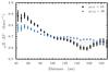 |
Fig. 7 Comparing the |
The single-molecule methods, either direct or parametric, are limited by our ability to recover the kinetic temperature with precision. Uncertainties on the kinetic temperature come from different origins: thermal noise, incomplete thermalisation of the observed spectral lines, absolute calibration accuracy, and in the parametric model, inadequacy of the model. Thermal noise can be overcome by sufficient integration time. Incomplete thermalisation is a complex problem, and will in general require multi-line transition to be evaluated. However, in the case of CO, the critical densities are low, and we expect the CO lines to be very close to thermalisation. Absolute calibration will place an ultimate limit on our capabilities of measuring the turbulence.
We derive in Appendix B the effect of the uncertainty on the kinetic temperature on the derivation of the turbulence,
where ℳ is the Mach number of the turbulent broadening. The left panel of Fig. 8 shows, in the absence of any error in the measurement of the line width, the relative error in vturb as a function of relative error in Tkin for CO (assuming μ = 28). We note that as errors in ΔV have been neglected, Fig. 8a underestimates the precision in Tkin necessary to detect vturb.
Previous measurements from the Plateau de Bure Interferometer (PdBI) and the Sub-Millimetre Array (SMA) have typical flux calibrations of ~10% and ~20% respectively (Hughes et al. 2011; Guilloteau et al. 2012), therefore we estimate that these can only directly detect vturb at 3σ when vturb≳ 0.16cs and ≳0.26 cs, respectively. Our current ALMA experiment has a calibration accuracy of 7–10%, thus is sensitive to vturb≳ 0.2 cs for the turbulence not to be consistent with 0 m s-1 to 5σ. Ultimately, ALMA is expected to reach a flux calibration of ≈3%, which will translate into a limit of vturb≳0.07 cs for a ≥3σ detection.
However, the flux calibration does not affect the precision to which widths can be measured. The resulting errors on turbulence and temperature derived in the co-spatial method are given by, ![\begin{eqnarray} &&\frac{\delta v_{\rm turb}}{v_{\rm turb}} = \frac{1}{\mu_{\rm B} - \mu_{\rm A}} \, \frac{\delta \Delta V}{\Delta V} \sqrt{\,\left(\mu_{\rm A} + \frac{\mu_{\rm H}}{\mathcal{M}^2} \right)^2 + \frac{1}{x^2} \, \left( \mu_{\rm B} + \frac{\mu_{\rm H}}{\mathcal{M}^2} \right)^2}, \\[6mm] &&\frac{\delta T}{T} = \frac{2 \mu_{\rm A} \mu_{\rm B}}{\mu_{\rm B} - \mu_{\rm A}} \frac{\delta \Delta V}{\Delta V} \sqrt{\,\left( \frac{\mathcal{M}^2}{\mu_{\rm H}} + \frac{1}{\mu_{\rm A}} \right)^2 + \frac{1}{x^2} \, \left( \frac{\mathcal{M}^2}{\mu_{\rm H}} + \frac{1}{\mu_{\rm B}}\right)^2}, \end{eqnarray}](/articles/aa/full_html/2016/08/aa28550-16/aa28550-16-eq155.png) where x is a scaling factor between the relative errors on the two line widths,
where x is a scaling factor between the relative errors on the two line widths,  (11)See Appendix B for the complete derivation.
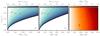 |
Fig. 8 Limitations in determining vturb and Tkin from the two direct methods. Panels a) and b) show the relative error in vturb for a given (vturb/cs) as a function of the temperature a) and line width b) corresponding to the direct method with a known excitation temperature and the co-spatial method, respectively. Panel c) shows the relative error in Tkin from the co-spatial method as a function of relative error in line width. The left panel does not take into account errors in the line width. The dashed contour lines show 10, 5, and 3σ limits. |
Figure 8b shows the relative error on vturb assuming the molecular masses of CN and CS (26 and 44 respectively) and that the relative errors on both lines are the same, x = 1. Figure 8c shows the limits of this method in determining Tkin. For the observations presented in this paper, we have a precision in the measurement of the line width of ≈0.3% for both CO and CN, and ≈1% for CS (hence x ≈ 0.33).
Parametric models typically return much lower formal errors on vturb than direct methods (for example, we find relative errors in Sect. 3.5 of about 5%). However, this is only a result of the imposed prior on the shape of the radial dependency of the temperature and turbulent width, which can lead to a significant bias that is not accounted for in the analysis. In any case, these parametric models suffer from the same fundamental limits due to thermalisation and absolute calibration as the single-molecule direct method.
4.4. Comparison with other observations, disks and simulations
Turbulence in TW Hya was modelled previously by Hughes et al. (2011) using 40 m s-1 resolution SMA observations of CO (3–2). Using a model-fitting approach the authors found an upper limit of vturb≲ 40 m s-1 corresponding to ≲0.1 cs, considerably lower than the values plotted in Fig. 5. The temperature profile assumed for their parametric model was warmer than found in this work, with the authors quoting T100 = 40 K and eT = 0.4 compared to our values of T100 = 34.5 ± 0.1 K and eT = 0.492 ± 0.002 (see Fig. 9). This warmer profile is sufficient to account for any difference in the resulting vturb. Both measurements are fundamentally limited by the absolute calibration uncertainty, and only imply vturb< 0.23 cs (SMA data) or <0.16 cs (our ALMA data).
Other disks have also been the subject of investigations of vturb. DM Tau, MWC 480 and LkCa 15 have yielded higher velocities of ≲100−200 m s-1 (≲0.3−0.5cs) (Dartois et al. 2003; Piétu et al. 2007) which are sufficiently high to be detected by the PdBI. However, the velocity resolution of the observations was about 200 m s-1 resulting in a poorly constrained total line width that may result in overestimating vturb. The effect of the spectral resolution was accounted for in the more recent measurement of DM Tau by Guilloteau et al. (2012) using the heavier molecule CS, who found vturb≃0.3−0.4 cs. More recently Flaherty et al. (2015) used parametric modelling of multiple CO isotopologue transitions to infer vturb≲0.04 cs in HD 163296.
We must consider the effect of flux calibration on all methods involving a single line measurement, however. Every method will constrain the local line width using some combination of diagnostics, such as the broadening of channel images or the peak-to-trough ratio of the integrated spectra. Each method will recover this line width to its own precision (depending particularly on the functional form imposed on the spatial dependency of this line width). However, when the uncertainty on the local line width is known, Eq. (8) can be applied to propagate the error that is due to this uncertainty and to the absolute calibration precision to the turbulent component of the line width. Application to the results of Hughes et al. (2011) and Flaherty et al. (2015) yields upper limits of vturb< 0.23 cs and <0.16 cs respectively, more similar to what we measure here. The vturb value found for DM Tau is considerably higher than limits imposed by the flux calibration (≈10%). Given consideration of the observed limits, this suggests that the disk of DM Tau is more turbulent than those of TW Hya and HD 163296.
Comparisons with numerical simulations also provide a chance to distinguish between turbulent mechanisms. Simon et al. (2015) used an ensemble of shearing-box magnetohydrodynamic (MHD) simulations coupled with radiative transfer modelling to predict the velocity dispersion traced by CO emission in a proto-typical T-Tauri disk pervaded by MRI. The authors found that molecular emission would trace a transition region between the dead-zone and the turbulent atmosphere, showing velocity dispersions of between 0.1 and 0.3 cs, almost identical to the range found in TW Hya. Flock et al. (2015) ran similar, but global, models of a magnetorotationally instable (MRI) active disk, finding velocity dispersions of vturb≈ 40–60 m s-1 near the midplane, rising to 80–120 m s-1 higher above the midplane, again consistent with the values found in TW Hya. A comparison with the α viscosity models is more complex because the relation between vturb and α depends on the nature of the viscosity, with vturb ranging between a few αcs and  (Cuzzi et al. 2001).
A vertical dependence of vturb, as found in Flock et al. (2015), is a typical feature of MRI-driven turbulence and may provide a discriminant between other models of turbulent mixing. In addition to the parametric model that found different temperatures for all three molecules, CO and CN yielded different Tex values from the line profile fitting and the simultaneous method failed under the assumption that CN and CS are co-spatial. These pieces of evidence suggest that CO, CN, and CS each trace distinct vertical regions in the disk, potentially providing a possibility of tracing a vertical gradient in vturb. With the current uncertainties on the temperatures for the three molecules we are unable to distinguish any difference in vturb with height above the midplane.
Cleeves et al. (2015) have modelled the ionisation structure of TW Hya using observations of key molecular ions HCO+ and N2H+, concluding that the disk may have a large MRI-dead zone extending to ~50−65 au. An observable feature of such a dead zone would be a sharp decrease in the velocity dispersion at this radius. Our data lack the spatial resolution and sensitivity to reliably trace the gas turbulent motions in the inner ~40 au where this feature may be more prominent. However, the power-law analysis indicates that the vturbvalues increase with radius (exponent eδv< 0), in contrast with the direct measurements. This difference may be due to the effect of such a less turbulent inner region that is ignored in the direct method, but must be fitted in the power-law analysis.
 |
Fig. 9 Comparing the temperature structure of our fits and that of Hughes et al. (2011) shown in grey. Hughes et al. (2011) observed CO (3–2) with the SMA with a flux calibration of ~20%. Work from this paper uses CO (2–1) with ALMA, which has a flux calibration of ≈7%. |
Future observations will improve this analysis: to improve the accuracy of the vturb determination with this direct method, a well-constrained thermal structure is crucial. This can be attained with observations of multiple transitions of the same molecule. Furthermore, for more highly inclined systems, a better understanding of the effect of beam smearing on the velocity dispersion is paramount. This can be achieved with smaller beamsizes that resolve a smaller shear component. Of the observed species, CS currently provides the best opportunity to probe velocity dispersions closer to the midplane, while we have demonstrated that the ensemble of CO, CN and CS can allow additionally for the determination of the vertical dependence of vturb. Despite all these improvements, direct measures of turbulence will ultimately be limited by the flux calibration of the interferometers with a sensitivity of ≈0.1 cs for ALMA’s quoted 3% accuracy.
5. Conclusion
We have discussed several methods of obtaining the turbulent velocity dispersion in the disk of TW Hya using CO, CN and CS rotational emission with a view to complementing the commonly used parametric modelling approach. Guided by previous models of TW Hya, the direct method yields vturb values that strongly depend on the radius of the disk, reaching ≈150 m s-1 at 40 au, dropping to a nearly constant ≈50 m s-1 outside 100 au for all three tracers. As a function of local soundspeed, CO and CN displayed a near constant vturb~ 0.2 cs. However, the analysis of the possible sources of errors shows that these numbers should most likely be interpreted as upper limits.
Direct or parametric methods using a single molecule are limited by a poor knowledge of the thermal structure of the disk. Additional transition lines will provide a more accurate determination of the temperature, but this is ultimately limited by the flux calibration of ALMA. With an expected error of at least 3% on the flux calibration, we estimate that a firm detection of turbulent broadening is only possible if vturb/cs ≳ 0.1 through this direct method. The co-spatial method can potentially overcome this absolute calibration problem, but it requires two co-spatial tracers of sufficient abundance to have strong emission. Tracing vturb close to the midplane will be considerably more challenging because it requires a strong detection of o-H2D+ and another molecule residing in the midplane, such as N2D+.
Acknowledgments
We thank the referee, whose helpful comments have improved this manuscript. R.T. is a member of the International Max Planck Research School for Astronomy and Cosmic Physics at the University of Heidelberg, Germany. D.S. and T.B. acknowledge support by the Deutsche Forschungsgemeinschaft through SPP 1385: “The first ten million years of the solar system a planetary materials approach” (SE 1962/1–3) and SPP 1833 “Building a Habitable Earth” (KL 1469/13-1), respectively. This research made use of System. This paper makes use of the following ALMA data: ADS/JAO.ALMA#2013.1.00387.S. ALMA is a partnership of ESO (representing its member states), NSF (USA) and NINS (Japan), together with NRC (Canada), NSC and ASIAA (Taiwan), and KASI (Republic of Korea), in cooperation with the Republic of Chile. The Joint ALMA Observatory is operated by ESO, AUI/NRAO and NAOJ. This work was supported by the National Programs PCMI and PNPS from INSU-CNRS.
References
- Brinch, C., & Hogerheijde, M. R. 2010, A&A, 523, A25 [NASA ADS] [CrossRef] [EDP Sciences] [Google Scholar]
- Cleeves, L. I., Bergin, E. A., & Harries, T. J. 2015, ApJ, 807, 2 [NASA ADS] [CrossRef] [Google Scholar]
- Cuzzi, J. N., Hogan, R. C., Paque, J. M., & Dobrovolskis, A. R. 2001, ApJ, 546, 496 [NASA ADS] [CrossRef] [Google Scholar]
- Dartois, E., Dutrey, A., & Guilloteau, S. 2003, A&A, 399, 773 [NASA ADS] [CrossRef] [EDP Sciences] [Google Scholar]
- Dutrey, A., Wakelam, V., Boehler, Y., et al. 2011, A&A, 535, A104 [NASA ADS] [CrossRef] [EDP Sciences] [Google Scholar]
- Flaherty, K. M., Hughes, A. M., Rosenfeld, K. A., et al. 2015, ApJ, 813, 99 [NASA ADS] [CrossRef] [Google Scholar]
- Flock, M., Ruge, J. P., Dzyurkevich, N., et al. 2015, A&A, 574, A68 [NASA ADS] [CrossRef] [EDP Sciences] [Google Scholar]
- Gorti, U., Hollenbach, D., Najita, J., & Pascucci, I. 2011, ApJ, 735, 90 [NASA ADS] [CrossRef] [Google Scholar]
- Guilloteau, S., Dutrey, A., Wakelam, V., et al. 2012, A&A, 548, A70 [NASA ADS] [CrossRef] [EDP Sciences] [Google Scholar]
- Henning, T., & Meeus, G. 2011, Dust Processing and Mineralogy in Protoplanetary Accretion Disks, ed. P. J. V. Garcia (Chicago: University of Chicago Press), 114 [Google Scholar]
- Hughes, A. M., Wilner, D. J., Andrews, S. M., Qi, C., & Hogerheijde, M. R. 2011, ApJ, 727, 85 [NASA ADS] [CrossRef] [Google Scholar]
- Lenz, D. D., & Ayres, T. R. 1992, PASP, 104, 1104 [NASA ADS] [CrossRef] [Google Scholar]
- Müller, H. S. P., Thorwirth, S., Roth, D. A., & Winnewisser, G. 2001, A&A, 370, L49 [NASA ADS] [CrossRef] [EDP Sciences] [Google Scholar]
- Piétu, V., Dutrey, A., & Guilloteau, S. 2007, A&A, 467, 163 [NASA ADS] [CrossRef] [EDP Sciences] [Google Scholar]
- Pringle, J. E. 1981, ARA&A, 19, 137 [NASA ADS] [CrossRef] [Google Scholar]
- Qi, C., Ho, P. T. P., Wilner, D. J., et al. 2004, ApJ, 616, L11 [NASA ADS] [CrossRef] [Google Scholar]
- Qi, C., Öberg, K. I., Wilner, D. J., et al. 2013, Science, 341, 630 [NASA ADS] [CrossRef] [PubMed] [Google Scholar]
- Roberge, A., Weinberger, A. J., & Malumuth, E. M. 2005, ApJ, 622, 1171 [NASA ADS] [CrossRef] [Google Scholar]
- Rosenfeld, K. A., Qi, C., Andrews, S. M., et al. 2012, ApJ, 757, 129 [NASA ADS] [CrossRef] [Google Scholar]
- Rosenfeld, K. A., Andrews, S. M., Hughes, A. M., Wilner, D. J., & Qi, C. 2013, ApJ, 774, 16 [NASA ADS] [CrossRef] [Google Scholar]
- Shakura, N. I., & Sunyaev, R. A. 1973, A&A, 24, 337 [NASA ADS] [Google Scholar]
- Simon, J. B., Hughes, A. M., Flaherty, K. M., Bai, X.-N., & Armitage, P. J. 2015, ApJ, 808, 180 [NASA ADS] [CrossRef] [Google Scholar]
- Skatrud, D. D., De Lucia, F. C., Blake, G. A., & Sastry, K. V. L. N. 1983, J. Mol. Spectr., 99, 35 [Google Scholar]
- Testi, L., Birnstiel, T., Ricci, L., et al. 2014, in Dust Evolution in Protoplanetary Disks, eds. H. Beuther, C. Dullemond, R. Klessen, & T. Henning, 339 [Google Scholar]
Appendix A: CN hyperfine components
New frequencies for CN N = 2−1 transitions.
Here we present the relative offsets of the CN N = (2−1) hyperfine components used in the paper. The old and new values are given in Table. A.1.
Appendix B: Error derivations
In this section, we discuss the uncertainties arising from the line profile fitting and their subsequent propagation into the derivation of vturb.
Appendix B.1: Uncertainties from line profile fitting
The uncertainty of a Gaussian line parameter X is derived from Eq. (1) from Lenz & Ayres (1992),  (B.1)where CX is a coefficient of order 1, given in Table 1 by the same authors. σ is the noise per channel of width δv, and Tp the peak intensity of the Gaussian, while ΔV is its FWHM. For the line width, CX ≈ 0.6. The simultaneous fit of the opacity slightly reduces this number.
In our observations, in one channel of 30.5 kHz, or about 40 m s-1, we have a typical rms noise of about 6–7 mJy/beam, which translates into about 0.5–0.7 K at the angular resolution of our data (around 0.5″). CO has line widths of around 300 m s-1, and a peak intensity of around 40 K, yielding errors on the line widths of about 2.7 m s-1 (1% precision) for each beam. The CN peak typical brightness is lower, about 20 K, but CN has several hyperfine components, so that the precision obtained from CN is only 1.5 times lower than from CO. For CS, the peak brightness is instead about 10 K, leading to a precision of about 4%.
The error is further reduced by azimuthal averaging because the number of independent beams increases as  . At 100 au, we average about 22 beams, and the gain is about a factor 4.7. Thus the final precision on the line widths on the azimuthal average is about 1% for CS and a factor 2 (3) better for CN (CO).
It is also worth noting that for a given integration time, the precision does not depend on the selected spectral resolution, provided it is sufficient to sample the line shape. Figure B.1 demonstrates the incurred bias when the line is not sufficiently resolved.
 |
Fig. B.1 Effect of spectrally resolving a line on the determination of ΔV. For the data presented in this paper, CO and CN have a maximum ratio of 0.21 and CS has 0.25, resulting in fractional errors for ΔV of ≈2% and 3.5%, respectively. |
Appendix B.2: Direct turbulent velocity dispersion
Assuming Tkin is known, the turbulent velocity component vturb is given by  (B.2)We assume δT ≫ δΔV, therefore the uncertainty on vturb is
  Dividing by vturb to obtain the relative error gives
  (B.5)From rearranging Eq. (B.2) for ΔV,
  we can be substitute this into Eq. (B.5) to yield
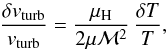
 ![\appendix \setcounter{section}{2} \begin{eqnarray} \frac{\delta v_{\rm turb}}{v_{\rm turb}} &=& \frac{k}{\mu m_{\rm p}} \, \left( \frac{2kT}{m_{\rm p}} \left[\frac{\mathcal{M}^2}{\mu_{\rm H}} + \frac{1}{\mu}\right] - \frac{2kT}{\mu m_{\rm p}} \right)^{-1} \delta T, \\ &=& \frac{2\mu_{\rm H}}{\mu \mathcal{M}^2} \, \frac{\delta T}{T}\cdot \end{eqnarray}](/articles/aa/full_html/2016/08/aa28550-16/aa28550-16-eq208.png)
Appendix B.3: Co-spatial kinetic temperature
The kinetic temperature and its associated uncertainty are  We assume that the relative errors on the line width are proportional to one another such that,
  (B.12)where x scales the relative errors if they are not the same; Fig. 8 uses x = 1. Substituting these into the Eq. (B.11) yields
 ![\appendix \setcounter{section}{2} \begin{eqnarray} \delta T &=& 2\,\frac{m_{\rm p}}{2k} \frac{\mu_{\rm A} \mu_{\rm B}}{\mu_{\rm B} - \mu_{\rm A}} \sqrt{\,\left( \Delta V_{\rm A}^2 \cdot \frac{\delta \Delta V}{\Delta V}\right)^2 + \, \left( \frac{\Delta V_{\rm B}^2}{x} \cdot \frac{\delta \Delta V}{\Delta V}\right)^2}, ~~~~~~~~~~~~~~~~~~~~~~~~~~~~~~~~\\[2mm] &=& 2\,\frac{m_{\rm p}}{2k} \frac{\mu_{\rm A} \mu_{\rm B}}{\mu_{\rm B} - \mu_{\rm A}} \frac{\delta \Delta V}{\Delta V} \sqrt{\Delta V_{\rm A}^4 + \frac{\Delta V_{\rm B}^4}{x^2}}\cdot~~~~~~~~~~~~~~~~~~~~~~~~~~~~~~~~ \end{eqnarray}](/articles/aa/full_html/2016/08/aa28550-16/aa28550-16-eq211.png)
Substituting for  and
and  from Eq. (B.7) and rearranging for the relative uncertainty on T,
  (B.15)
Appendix B.4: Co-spatial turbulent velocity dispersion
This can be repeated with the turbulent velocity dispersion:  Substituting for the relative line widths from Eq. (B.12) and for vturb from Eq. (B.2) gives
  (B.18)Rearranging Eq. (B.7) yields
  (B.19)which can be substituted into Eq. (B.18). After some rearranging, we find
 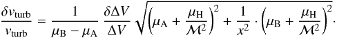 (B.20)
Appendix C: Observations
 |
Fig. C.1 Integrated intensity maps of CN including all hyperfine components, left, and CS, right. Contours are 10% of the peak value. No azimuthal structure is seen within the noise for either line. |
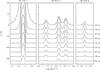 |
Fig. C.2 Azimuthally averaged spectra for the three emission lines: CO, left; CN, centre; and CS, right. The radial sampling is roughly one beam size. |
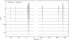 |
Fig. C.3 Full compliment of CN = (2–1) hyperfine components as described in Table A.1. Each line is an azimuthal average taken at a radius as shown in Fig. C.2, roughly one beam size in distance. |
We describe the observational data. Figure C.1 shows the integrated intensities of CN (including all hyperfine components) and CS clearly demonstrating the lack of azimuthal structure, as with CO which is identical to previous studies.
Examples of the spectra used for the analysis are shown in Fig. C.2. The full complement of hyperfine components is shown in Fig. C.3.
All Tables
All Figures
|
Fig. 1 Example spectra of CO (left), CN (centre) and CS (right). All spectra are from a pixel removed by 1″ from the centre. This example only shows three hyperfine components for CN. The red lines show example fits to the data, CO being an optically broadened Gaussian, CN the ensemble of Gaussians, one for each hyperfine component, and CS a pure, optically thin Gaussian. Note that the spectra are Nyquist sampled in velocity. |
| In the text | |
|
Fig. 2 Measured line widths (black) and those corrected for the Keplerian shear component (blue) for CO (left), CN (centre) and CS (right). All three lines are subject to the same Keplerian shear component. The uncertainties include an uncertainty on the inclination of the disk of ±2° as described in Eq. (2). The solid yellow lines show the line widths from the global fit. |
| In the text | |
|
Fig. 3 Radial profile of the derived T values (in blue) used for calculating the thermal broadening component of the line width for CO (left), CN (centre) and CS and CN assuming co-spatiality (right). For CO and CN this is Tex while for CS this is Tkin. The black line shows the upper limit Tkin that would fully account for the total line width in the absence of turbulent broadening. Outside 140 au, the derived Tkin exceeds |
| In the text | |
|
Fig. 4 Effect of a temperature dispersion on the accuracy of the measurement of ℳ. The colouring shows how well an input ℳ value can be recovered from a line profile that is the summation of lines at differing temperatures described by δT. |
| In the text | |
|
Fig. 5 Radial profiles of the turbulent width in m s-1, top row, and as a function of local sound speed, bottom row. The blue dots show the results of the direct method, where the CO and CN lines were assumed to be fully thermalised, and CS to be co-spatial with CN to derive a Tkin value. Yellow solid lines show the results from the global fit where the total line width was fit for, while dashed grey lines show the global fit where vturb was fit for individually. The 1σ uncertainties are shown as bars for the direct method and as shaded regions for the lines. A representative error associated with the flux calibration of 7% at 80 au is shown in the top left corner of all panels. |
| In the text | |
|
Fig. 6 2D distribution of vturb for all three lines: CO (left), CN (centre), and the combination of CN and CS assuming co-spatiality, therefore sharing the same Tex and vturb values (right). The values are masked outside 180 au and within 40 au. The beam size is shown in the bottom left corner for each line, and the major and minor axes are denoted by the central cross, aligned with the x- and y-axes, respectively. At the distance of TW Hya, 1″ ≈ 54 au. The azimuthal asymmetry see in the inner disk is an artefact of a purely radial subtraction of the beam-smearing component discussed in Sect. 3.2. |
| In the text | |
|
Fig. 7 Comparing the |
| In the text | |
|
Fig. 8 Limitations in determining vturb and Tkin from the two direct methods. Panels a) and b) show the relative error in vturb for a given (vturb/cs) as a function of the temperature a) and line width b) corresponding to the direct method with a known excitation temperature and the co-spatial method, respectively. Panel c) shows the relative error in Tkin from the co-spatial method as a function of relative error in line width. The left panel does not take into account errors in the line width. The dashed contour lines show 10, 5, and 3σ limits. |
| In the text | |
|
Fig. 9 Comparing the temperature structure of our fits and that of Hughes et al. (2011) shown in grey. Hughes et al. (2011) observed CO (3–2) with the SMA with a flux calibration of ~20%. Work from this paper uses CO (2–1) with ALMA, which has a flux calibration of ≈7%. |
| In the text | |
|
Fig. B.1 Effect of spectrally resolving a line on the determination of ΔV. For the data presented in this paper, CO and CN have a maximum ratio of 0.21 and CS has 0.25, resulting in fractional errors for ΔV of ≈2% and 3.5%, respectively. |
| In the text | |
|
Fig. C.1 Integrated intensity maps of CN including all hyperfine components, left, and CS, right. Contours are 10% of the peak value. No azimuthal structure is seen within the noise for either line. |
| In the text | |
|
Fig. C.2 Azimuthally averaged spectra for the three emission lines: CO, left; CN, centre; and CS, right. The radial sampling is roughly one beam size. |
| In the text | |
|
Fig. C.3 Full compliment of CN = (2–1) hyperfine components as described in Table A.1. Each line is an azimuthal average taken at a radius as shown in Fig. C.2, roughly one beam size in distance. |
| In the text | |
Current usage metrics show cumulative count of Article Views (full-text article views including HTML views, PDF and ePub downloads, according to the available data) and Abstracts Views on Vision4Press platform.
Data correspond to usage on the plateform after 2015. The current usage metrics is available 48-96 hours after online publication and is updated daily on week days.
Initial download of the metrics may take a while.