| Issue |
A&A
Volume 577, May 2015
|
|
|---|---|---|
| Article Number | A31 | |
| Number of page(s) | 6 | |
| Section | Astrophysical processes | |
| DOI | https://doi.org/10.1051/0004-6361/201424490 | |
| Published online | 27 April 2015 | |
The Ep − Eiso relation and the internal shock model
1
UPMC-CNRS, UMR 7095, Institut d’Astrophysique de Paris,
75014
Paris,
France
e-mail:
mochko@iap.fr
2
Racah Institute of Physics, The Hebrew University of
Jerusalem, 91904
Jerusalem,
Israel
3
APC, Université Paris Diderot, CNRS/IN2P3, CEA/Irfu, Observatoire
de Paris, Sorbonne Paris
Cité, 75025
Paris,
France
Received: 27 June 2014
Accepted: 6 October 2014
Context. The validity of the Ep − Eiso correlation in gamma-ray bursts and the possibility of explaining the prompt emission with internal shocks are highly debated questions.
Aims. We study whether the Ep − Eiso correlation can be reproduced if internal shocks are indeed responsible for the prompt emission, or conversely, if the correlation can be used to constrain the internal shock scenario.
Methods. We developed a toy model where internal shocks are limited to the collision of only two shells. Synthetic burst populations were constructed for various distributions of the model parameters, such as the injected power in the relativistic outflow, the average Lorentz factor, and its typical contrast between the shells. These parameters can be independent or linked by various relations.
Results. Synthetic Ep − Eiso diagrams are obtained in the different cases and compared with the observed correlation. The reference observed correlation is the one defined by the BAT6 sample, a sample of Swift bursts almost complete in redshift and affected by well-known and reproducible instrumental selection effects. The comparison is then performed with a subsample of synthetic bursts that satisfy the same selection criteria as were imposed on the BAT6 sample. A satisfactory agreement between model and data can often be achieved, but only if several strong constraints are satisfied on both the dynamics of the flow and the microphysics that governs the redistribution of the shock-dissipated energy.
Key words: gamma-ray burst: general / radiation mechanisms: non-thermal / shock waves
© ESO, 2015
1. Introduction
The origin of the prompt emission of gamma-ray bursts (GRBs) is still debated. Temporal variability down to very short time-scales imposes that the emission comes directly from the relativistic outflow emitted by the central engine and not from its interaction with the circumburst medium (external origin; Sari & Piran 1997). But at least three possibilities remain for an internal origin: (i) dissipation below the photosphere that can modify the emerging thermal spectrum by inverse Compton scattering off energetic electrons (Rees & Mészáros 2005; Pe’er et al. 2005; Ryde et al. 2011; Giannios 2012; Beloborodov 2013); (ii) dissipation above the photosphere either of the flow kinetic energy by internal shocks (Rees & Meszaros 1994; Kobayashi et al. 1997; Daigne & Mochkovitch 1998); or (iii) in a magnetized ejecta through reconnection processes (McKinney & Uzdensky 2012; Yuan & Zhang 2012; Zhang & Zhang 2014). Many predictions on the light curves and spectra of GRBs can be made from internal shocks (Bosnjak & Daigne 2014). Several agree well with observations, but the shape of the expected synchrotron spectrum does not fit well, because it is too soft at low energy (Preece et al. 1998; Ghisellini et al. 2000; see however Derishev 2007; Daigne et al. 2011). Moreover, the necessary efficient transfer of dissipated energy to electrons has been disputed for a moderate magnetization of the flow σ> 0.1, where σ is the ratio of the Poynting flux to the particle rest energy flux (Mimica & Aloy 2010; Narayan et al. 2011).
Photospheric dissipation and reconnection models have been proposed to avoid these problems. Photospheric dissipation can take place through radiation mediated shocks (Levinson 2012; Keren & Levinson 2014), collisional heating (Beloborodov 2010), or reconnection, and then the main emission mechanism is not synchrotron.
If reconnection takes place above the photosphere, the emission should again come from the synchrotron process, as it does for internal shocks with the same potential problems regarding the spectral shape. For photospheric and reconnection models few works have been dedicated to actually produce light curves that can be compared with data to test the temporal (and spectro-temporal) evolution of the models (see Zhang & Zhang 2014, however).
Scenarios for the prompt emission can be tested on their ability to reproduce not only light curves and spectra of individual events, but also the properties of the GRB population as a whole. An example is the Ep − Eiso (or Amati) relation (Amati et al. 2002) or Ep − Eγ (or Ghirlanda) relation (Ghirlanda et al. 2004), where Eγ is the true energy release in gamma-rays.
Similarly to the possibility of explaining the prompt emission of GRBs with internal shocks, the validity of the Amati relation has been disputed with indications that it might be, at least partially, the result of selection effects (Nakar & Piran 2005; Band & Preece 2005; Butler et al. 2007; Shahmoradi & Nemiroff 2011). However, several studies, aimed at quantifying these selection effects for different detectors, have shown that even if instrumental biases contribute to shaping the distribution of GRBs in the Ep − Eiso plane, they cannot be fully responsible for the observed correlation, which therefore must also have a physical origin (Ghirlanda et al. 2008, 2012a; Nava et al. 2008).
Attempts have been made to interpret the Ghirlanda relation as the result of viewing-angle effects (Levinson & Eichler 2005) or of similar comoving-frame properties for all GRBs, with correlations being the results of the spread in the jet Lorentz factor (Ghirlanda et al. 2012b). The estimate of the collimation-corrected energy Eγ requires measuring the jet break-time from late-time afterglow observations and the knowledge of the density of the circum-burst medium. Depending on the assumed density profile, the slope of the Ep − Eγ correlation is around 0.7 for a homogeneous density profile and around 1 for a wind-like density profile (Nava et al. 2006). In both cases the slope is steeper than the slope of the Amati correlation. The consistency between the Ep − Eγ and Ep − Eiso correlations and their different slopes and scatters can be explained by assuming that the jet opening angle is anticorrelated with the energy (Ghirlanda et al. 2005, 2013).
In this paper we focus on the Ep − Eiso correlation. We especially wish to determine (i) under which conditions the internal shock model would be able to account for it; and (ii) to examine whether these conditions are realistic and can indeed be satisfied. To do this we also take into account the role of selection effects in the observed Ep − Eiso relation. While the lack of bursts with a high Eiso and a low Ep should have a physical origin, events with a low Eiso and a high Ep may escape detection, as discussed by Heussaff et al. (2013).
The paper is organized as follows: we describe in Sect. 2 the toy model we used to generate large populations of synthetic bursts with different assumptions on the model parameters and the possible links between them. We discuss in Sect. 3 the role of instrumental biases with the aim to construct a synthetic sample including selection effects similar to those affecting a reference sample of observed bursts. We then compare the Ep − Eiso relations defined by various synthetic populations with the relation defined by the reference sample. Our results are discussed in Sect. 4, which is also the conclusion.
2. Constructing a large population of synthetic bursts
2.1. Two-shell internal shock toy model
To generate a large number (up to 106) of synthetic bursts, we restricted the internal shock phase to the collision of only two shells. Obviously, using this simplified approach we loose most of the details of the burst temporal evolution, but we expect to preserve the main features of the energetics and the peak of the time-integrated spectrum, which we need to obtain the Ep − Eiso relation. This model has previously been presented in Barraud et al. (2005), and we summarize their main assumptions and equations here.
The two shells have respective masses and Lorentz factors (Mi, Γi with i = 1,2) and are produced over a total duration τ. We can then define the average power injected in the relativistic outflow 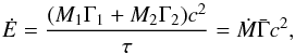 (1)where Ṁ = (M1 + M2) /τ and
  are the average mass-loss rate and Lorentz factor. The collision radius1 is
 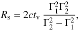 (2)where Γ2> Γ1 has been assumed and tv ≤ τ is a typical variability time scale over which the bulk of the energy is released, which is of about one second in long bursts (Nakar & Piran 2002). It is a key parameter in the internal shock model because it fixes the location of the shocks, and introducing it allows us to go somewhat beyond the basic two-shell model.
A fraction ϵe of the dissipated energy is transferred to electrons and radiated so that ![\begin{equation} E_{\rm iso}=\epsilon_{\rm e}\,E_{\rm diss}=\epsilon_{\rm e}\,\left[M_1 \Gamma_1+M_2 \Gamma_2-(M_1+M_2)\,\Gamma_{\rm f}\right]c^2 , \end{equation}](/articles/aa/full_html/2015/05/aa24490-14/aa24490-14-eq24.png) (3)where the final Lorentz factor after the two shells have merged is given by
(3)where the final Lorentz factor after the two shells have merged is given by 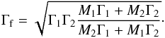 (4)The peak energy of the synchrotron spectrum is
  (5)where B and Γe are the post-shock magnetic field and electron Lorentz factor and
  . We obtain B and Γe using the redistribution parameters ϵe, ϵB and ζ (fraction of electrons that are accelerated)
  (6)where
  (7)is the post-shock density and
  (8)is the dissipated energy per unit mass in the comoving frame. Equations (7) and (8) lead to
  (9)with
  (10)If we additionally assume for simplicity that M1 = M2, the isotropic energy of the burst Eiso, its average luminosity ⟨ Liso ⟩ = Eiso/τ, and Ep can be simply expressed in terms of the model parameters. We have
  (11)and
  (12)where κ = Γ2/ Γ1 and f and ϕ are functions of κ only
 ![\begin{equation} \left\lbrace\begin{array}{ll} \! f(\kappa)&={(\sqrt{\kappa}-1)^2\over 1+\kappa}\\ \! \varphi(\kappa)&={\left[\left(\kappa^2-1\right)\,\left(1+1/\kappa\right)^2\right]\left(\kappa^{1/2} +\kappa^{-1/2}-2\right)^{5/2}\over \kappa^{1/2}+\kappa^{-1/2}}\cdot\\ \end{array}\right. \end{equation}](/articles/aa/full_html/2015/05/aa24490-14/aa24490-14-eq45.png) (13)
(13)
2.2. Monte Carlo approach
To generate an Ep − Eiso diagram that can be compared with observations we need to fix the following:
-
The distribution in redshift of the events: we adopted a burst rate that follows the star formation rate SFR3 of Porciani & Madau (2001), which increases at large z, in contrast to the cosmic SFR, which is probably declining. This accounts for the fact that the stellar population at large z appears to be more efficient in producing GRBs than at low z, so that the burst rate is not directly proportional to the SFR (Daigne et al. 2006; Kistler et al. 2009; Wanderman & Piran 2010; Butler et al. 2010).
-
The distribution of intrinsic duration τ: we adopted a log-normal distribution centered on τ = 8 s and checked a posteriori that the distribution of the duration of the detected bursts (including time dilation) agrees with the observed distribution for long GRBs (Paciesas et al. 1999). Similarly, we also adopted a log-normal distribution for the variability time-scale tv, so that the distribution of tv in detected bursts fits that of pulse widths (Nakar & Piran 2002).
-
The distribution of injected power Ė: we adopted a power law of index δ = −1.6, the value of δ being constrained in the interval −1.7 <δ< −1.5 to reproduce the Log N − Log P curve (Daigne et al. 2006). The upper limit Ėmax must be high enough to make the most energetic events that can exceed Eiso = 1054 erg, and we therefore took Ėmax = 3 × 1054 erg s-1 to account for the low efficiency of internal shocks
 (14)The lower limit Ėmin could be more than six orders of magnitude lower in bursts such as GRB 980425 and GRB 060218, but these events probably belong to a different population with its own distinct luminosity function (Virgili et al. 2009). For cosmological bursts Ėmin is weakly constrained by observations. We adopted Ėmin = 1052 erg s-1.
 -
The distributions of contrast κ = Γ2/ Γ1 and average Lorentz factor
 : the function ϕ(κ) in Eq. (13) rapidly increases with κ (approximately as κ5 for κ ~ 5) so that to avoid a too high dispersion in the Ep − Eiso relation, κ has to be confined within a relatively narrow interval. Unless otherwise stated, we adopted a normal distribution for κ, centered on κ = 5 with a standard deviation σκ = 1. For , we first assumed a uniform distribution from 100 to 400.
These choices correspond to a situation where the various model parameters are not correlated, but we also considered the possibility that some of them are directly linked. From studies of the rise time of the optical afterglow light curve it has been suggested for example, that the average Lorentz factor increases with burst luminosity as  (Liang et al. 2010; Ghirlanda et al. 2012b; Lü et al. 2012). In this work, we replaced the luminosity by the injected power and tested the relation
  (15)Other examples may consist to link the time scale tv or/and amplitude of the fluctuations of the Lorentz factor κ, to the average Lorentz factor
  , that is to assume that the flow becomes more chaotic when it is more relativistic. A first possibility, suggested by Eq. (12), would be to have
  (16)so that Ep ∝ Ė1/2ϕ(κ), directly yielding an Amati-like relation if ϕ(κ) does not vary too much. If additionally Eqs. (15) and (16) are satisfied together, variability and luminosity become connected with
  (17)implying that more luminous bursts will be both more relativistic and more variable (Reichart et al. 2001). Similarly, for the contrast in Lorentz factor we tested relations of the form
  (18)To compute Ep and Eiso, we finally fixed the values of the microphysics parameters: we took ϵe = 0.3, ϵB = 0.01 and ζ = 3 × 10⁻³ (i.e., ϵe/ζ = 100). The low value of ζ is required to guarantee that the emission occurs in the soft gamma-ray range.
3. Producing a synthetic Ep − Eiso diagram
3.1. Selection effects
After Ė, τ, , κ and the redshift were drawn according to the assumed distributions, we know for each synthetic burst Eiso (Eq. (11)) and Ep (Eq. (12)). Adopting a Band shape, we then computed the average flux and the fluence received on Earth in any given spectral interval. The low- and high-energy spectral indices were fixed to α = −1 and β = −2.5, which corresponds to the mean values of the observed distributions (Preece et al. 2000). Synchrotron emission in the fast-cooling regime instead predicts α = −1.5, but including the inverse-Compton process and a decreasing magnetic field behind the shocks can help to reduce the discrepancy (Derishev 2007; Daigne et al. 2011). Adopting α = −1.5 or −1 for the present study leads to very similar results.
To compare synthetic and observed Ep − Eiso sequences, we applied to the synthetic sample the very same selection effects that affect the observed sample. The main selection effects arise from the requirement to trigger the event, measure Eiso, Ep (which must fall inside the range of sensitivity of the instrument), and the redshift. The trigger threshold can be approximated as a threshold on the peak flux, while the need to perform a good spectral analysis broadly translates into a limit on the fluence (spectral threshold). Ghirlanda et al. (2008), Nava et al. (2008), and Nava et al. (2011) discussed these effects in detail, and derived for each of the relevant instruments the trigger and spectral thresholds. To lie above the spectral threshold is typically a more demanding request than to lie above the trigger threshold: to detect a burst is not a sufficient condition to derive Ep and Eiso from the spectral analysis.
Applying realistic selection effects to the synthetic sample is a hard task given the complexity of these selection effects and the fact that the observed bursts have been detected by different instruments, which introduce different thresholds. To study this properly, we compared our population of synthetic events with a sample with well-known and reproducible instrumental selection effects. We chose the BAT6 sample defined by Salvaterra et al. (2012). This is a subsample of the GRBs detected by BAT, which includes events with favorable observing conditions and with a peak flux Fpeak> 2.6 ph cm-2 s-1 in the 15−150 keV energy range. These requirements resulted in a sample of 58 GRBs with a redshift-completeness level of almost 90% (Salvaterra et al. 2012)2. The value of the flux threshold was chosen to reach a good compromise between redshift completeness and number of events, that is, still high enough to perform statistical studies. However, this value has another main advantage: it ensures that all the events detected above this threshold (which is much higher than the BAT trigger threshold) also lie above the spectral threshold. This means that for all bursts above that flux, the spectral analysis can be performed and the spectral threshold does not introduce strong effects. The dominant selection effect is the flux threshold, which for this sample is well known. For an appropriate comparison, we just applied the very same selection criteria to our sample of synthetic bursts.
From the whole sample of simulated bursts, we then selected only those with Fpeak> 2.6 ph cm-2 s-1 in the 15−150 keV energy range and compared their properties in the Ep − Eiso plane with the 50 events of the BAT6 sample with a measured redshift (the properties of the BAT6 sample in the Eiso − Ep plane have been studied in Nava et al. 2012). Our simple model only provides the average flux ⟨ F ⟩ of each synthetic burst however, which can be much lower than the peak flux in a highly variable event. To obtain an estimate of Fpeak we then applied a correction factor to ⟨ F ⟩. From inspecting long GRBs detected by BATSE, we found that in the plane Fpeak/ ⟨ F ⟩ vs. T90, these GRBs are distributed inside a triangular region. The lower and upper edges of this region are approximately described by the relations  and
and  , so that, to convert average fluxes into peak fluxes, we used the expression
 ![\begin{equation} {F_{\rm peak}\over {\langle F\rangle}}=\left[(1+z)\tau\right]^{[0.4+0.4(R-0.5)]}\!, \end{equation}](/articles/aa/full_html/2015/05/aa24490-14/aa24490-14-eq94.png) (19)where the random variable R is uniformly distributed between 0 and 1.
(19)where the random variable R is uniformly distributed between 0 and 1.
3.2. Results
The resulting Ep − Eiso synthetic sequences are shown in Fig.1 together with the observed BAT6 sample in the following cases (except ii):
-
(i)
no correlation between model parameters: a power-law fit of the resulting sequence yields
 keV with a dispersion of 0.4 in the Log Eiso − Log Ep plane.
 -
(ii)
 with a dispersion of 0.3 in
  : the predicted correlation is opposite to the observed correlation with
  .
. -
(iii)
is now only the lower value of for a given Ė, the maximum being
 and is uniformly distributed between these two limits. This agrees with the results of Hascoët et al. (2014), who recently reconsidered the estimates of from early optical afterglow observations. It leads to
  keV with a dispersion of 0.38. The resulting sequence is somewhat below the observed sequence. This can be corrected by reducing the fraction ζ of accelerated electrons even more. With ζ = 10-3 we derive
  keV with a dispersion of 0.4, which is the sequence represented in Fig. 1.
 -
(iv)
 ; more precisely and to avoid having tv>τ, we adopted
 ![\hbox{$t_{\rm v}={\rm min}\,[\tau,({\bar \Gamma}/200)^{-2}\ {\rm s}]$}](/articles/aa/full_html/2015/05/aa24490-14/aa24490-14-eq107.png) with a dispersion of 0.3 in Log tv. This gives
with a dispersion of 0.3 in Log tv. This gives  keV with a dispersion of 0.36. If, in addition to the condition on tv, we add the conditions on ( or
  ), we obtain very similar results.
 -
(v)
 ; we illustrate in Fig. 1 the choice
  (with
(with  ) and a dispersion of 0.1 in Log κ. We derive
  keV with a dispersion of 0.32.
In all these cases we also obtained the lower limit on the Lorentz factor from the annihilation of photons (corresponding to limit A of Lithwick & Sari 2001). The optically thick bursts are represented in cyan in Fig.1.
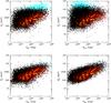 |
Fig. 1 Ep − Eiso relations with differents assumptions for the model parameters; black dots: whole synthetic population, except (in cyan) bursts that are optically thick as a result of photon-photon annihilation; red dots: detected bursts assuming a threshold of 2.6 ph cm-2 s-1 between 15 and 150 keV; yellow dots: observed BAT6 sample (Salvaterra et al. 2012). Upper left panel: no correlation among model parameters. Upper right panel: |

4. Discussion and conclusion
A satisfactory agreement with the observed Ep − Eiso relation can be achieved in several of the considered cases, but this is possible only if several strong constraints on the model parameters are satisfied:
-
A large portion of the dissipated energy has to be injected into a very small fraction of electrons. The value ζ = 3 × 10⁻³ (for ϵe = 0.3) we used should be considered as a lower limit however. Detailed hydro-calculations (Daigne & Mochkovitch 2000) show that Eqs. (7) and (8) both underestimate the density and the dissipated energy by a factor 3 to 5. This means that the required value for ζ can probably be increased by a factor of a few (possibly up to 10), but nevertheless remains very low.
-
The contrast κ between the maximum and minimum Lorentz factor should be restricted to a narrow interval because otherwise the function ϕ(κ) in Eq. (13) varies too much. This constraint can be somewhat relaxed if the fraction ζ of accelerated electrons does not remain constant, but rises together with the dissipated energy per unit mass e. Assuming, for example, ζ ∝ e, Eq. (9) would be replaced by Ep ∝ Γfρ1/2e1/2 (Bošnjak et al. 2009). The dependence of the peak energy on the contrast would be reduced, resulting in a larger allowed interval for κ.
-
If the average Lorentz factor increases as
 (with no other connection among the model parameters), the Ep − Eiso relation is lost. The peak energy is found to decrease with increasing Eiso. If is only a lower limit of for a given Ė, the Ep − Eiso relation can be recovered.
 -
When the time scale or amplitude of the Lorentz factor variability is correlated with the average Lorentz factor (i.e.,
 or
or  with ν ~ 0.5, satisfactory Ep − Eiso relations are obtained.
 -
In all cases, the dispersion of the intrinsic Ep − Eiso correlation (i.e., excluding instrument threshold) is higher than observed: the model accounts for the lack of bursts with a high Eiso and a low Ep, but selection effects are responsible for the suppression of bursts with a low Eiso and a high Ep. For case (v) the intrinscic Ep − Eiso relation is closest to the observed relation with
 keV and a dispersion of 0.39 in Log Ep.
These aforementioned conditions concern both (i) the dynamics of the flow and (ii) the redistribution of the dissipated energy:
-
(i)
In the first model we assumed that the parameters controlling the dynamics of the flow, Ė,
, κ, τ and tv were not correlated. This model provides a reasonable fit of the observed Ep − Eiso relation with a dispersion that might be too large, however. We then tested a few possible correlations:  , ,
, ,  , etc. Only the first correlation, if applied alone, does not yield acceptable results. Of all the constraints on the dynamics, the limited interval of acceptable values for the contrast in Lorentz factor appears to be the most restrictive.
 -
(ii)
The redistribution of the shock-dissipated energy should be efficient with ϵe = 0.1−0.3, and concern a very small fraction ζ = 10-3−10-2 of the electron population. This is probably the most severe constraint on the model, with the related question of the radiative contribution of the rest of the population with a quasi-thermal distribution.
The purpose of this short paper was to compare the predictions of the internal shock model with the Ep − Eiso relation, that is, assuming that internal shocks are responsible for the prompt emission of GRBs, are they able to account for the relation, and conversely, what are the constraints imposed on the model if the Ep − Eiso relation applies. We obtained constraints on both the dynamics of the flow and the microphysics, some of them appearing quite stringent. In all cases, except possibly when the contrast in Lorentz factor increases with average Lorentz factor of the flow, selection effects are required to exclude events with a low Ep and a high Eiso and reproduce the observed correlation.
The redshift completeness of the BAT6 sample has now been increased to 95% (Covino et al. 2013).
Acknowledgments
L.N. was supported by a Marie Curie Intra-European Fellowship of the European Communitys 7th Framework Programme (PIEF-GA-2013-627715), by an ERC advanced grant (GRB) and by the I-CORE Program of the PBC and the ISF (grant 1829/12). We also thank the French Program for High Energy Astrophysics (PNHE) for financial support.
References
- Amati, L., Frontera, F., Tavani, M., et al. 2002, A&A, 390, 81 [NASA ADS] [CrossRef] [EDP Sciences] [Google Scholar]
- Band, D. L., & Preece, R. D. 2005, ApJ, 627, 319 [NASA ADS] [CrossRef] [Google Scholar]
- Barraud, C., Daigne, F., Mochkovitch, R., & Atteia, J. L. 2005, A&A, 440, 809 [NASA ADS] [CrossRef] [EDP Sciences] [Google Scholar]
- Beloborodov, A. M. 2010, MNRAS, 407, 1033 [NASA ADS] [CrossRef] [Google Scholar]
- Beloborodov, A. M. 2013, ApJ, 764, 157 [NASA ADS] [CrossRef] [Google Scholar]
- Bosnjak, Z., & Daigne, F. 2014, A&A, 568, A45 [NASA ADS] [CrossRef] [EDP Sciences] [Google Scholar]
- Bošnjak, Ž., Daigne, F., & Dubus, G. 2009, A&A, 498, 677 [NASA ADS] [CrossRef] [EDP Sciences] [Google Scholar]
- Butler, N. R., Kocevski, D., Bloom, J. S., & Curtis, J. L. 2007, ApJ, 671, 656 [NASA ADS] [CrossRef] [Google Scholar]
- Butler, N. R., Bloom, J. S., & Poznanski, D. 2010, ApJ, 711, 495 [NASA ADS] [CrossRef] [Google Scholar]
- Covino, S., Melandri, A., Salvaterra, R., et al. 2013, MNRAS, 432, 1231 [NASA ADS] [CrossRef] [Google Scholar]
- Daigne, F., & Mochkovitch, R. 1998, MNRAS, 296, 275 [NASA ADS] [CrossRef] [Google Scholar]
- Daigne, F., & Mochkovitch, R. 2000, A&A, 358, 1157 [NASA ADS] [Google Scholar]
- Daigne, F., Rossi, E. M., & Mochkovitch, R. 2006, MNRAS, 372, 1034 [NASA ADS] [CrossRef] [Google Scholar]
- Daigne, F., Bošnjak, Ž., & Dubus, G. 2011, A&A, 526, A110 [NASA ADS] [CrossRef] [EDP Sciences] [Google Scholar]
- Derishev, E. V. 2007, Ap&SS, 309, 157 [NASA ADS] [CrossRef] [Google Scholar]
- Ghirlanda, G., Ghisellini, G., & Lazzati, D. 2004, ApJ, 616, 331 [NASA ADS] [CrossRef] [Google Scholar]
- Ghirlanda, G., Ghisellini, G., & Firmani, C. 2005, MNRAS, 361, L10 [NASA ADS] [Google Scholar]
- Ghirlanda, G., Nava, L., Ghisellini, G., Firmani, C., & Cabrera, J. I. 2008, MNRAS, 387, 319 [NASA ADS] [CrossRef] [Google Scholar]
- Ghirlanda, G., Ghisellini, G., Nava, L., et al. 2012a, MNRAS, 422, 2553 [NASA ADS] [CrossRef] [Google Scholar]
- Ghirlanda, G., Nava, L., Ghisellini, G., et al. 2012b, MNRAS, 420, 483 [NASA ADS] [CrossRef] [Google Scholar]
- Ghirlanda, G., Ghisellini, G., Salvaterra, R., et al. 2013, MNRAS, 428, 1410 [NASA ADS] [CrossRef] [EDP Sciences] [Google Scholar]
- Ghisellini, G., Celotti, A., & Lazzati, D. 2000, MNRAS, 313, L1 [NASA ADS] [CrossRef] [Google Scholar]
- Giannios, D. 2012, MNRAS, 422, 3092 [NASA ADS] [CrossRef] [Google Scholar]
- Hascoët, R., Beloborodov, A. M., Daigne, F., & Mochkovitch, R. 2014, ApJ, 782, 5 [NASA ADS] [CrossRef] [Google Scholar]
- Heussaff, V., Atteia, J.-L., & Zolnierowski, Y. 2013, A&A, 557, A100 [NASA ADS] [CrossRef] [EDP Sciences] [Google Scholar]
- Keren, S., & Levinson, A. 2014, ApJ, 789, 128 [NASA ADS] [CrossRef] [Google Scholar]
- Kistler, M. D., Yüksel, H., Beacom, J. F., Hopkins, A. M., & Wyithe, J. S. B. 2009, ApJ, 705, L104 [NASA ADS] [CrossRef] [Google Scholar]
- Kobayashi, S., Piran, T., & Sari, R. 1997, ApJ, 490, 92 [NASA ADS] [CrossRef] [Google Scholar]
- Levinson, A. 2012, ApJ, 756, 174 [NASA ADS] [CrossRef] [Google Scholar]
- Levinson, A., & Eichler, D. 2005, ApJ, 629, L13 [NASA ADS] [CrossRef] [Google Scholar]
- Liang, E.-W., Yi, S.-X., Zhang, J., et al. 2010, ApJ, 725, 2209 [NASA ADS] [CrossRef] [Google Scholar]
- Lithwick, Y., & Sari, R. 2001, ApJ, 555, 540 [NASA ADS] [CrossRef] [Google Scholar]
- Lü, J., Zou, Y.-C., Lei, W.-H., et al. 2012, ApJ, 751, 49 [NASA ADS] [CrossRef] [Google Scholar]
- McKinney, J. C., & Uzdensky, D. A. 2012, MNRAS, 419, 573 [Google Scholar]
- Mimica, P., & Aloy, M. A. 2010, MNRAS, 401, 525 [NASA ADS] [CrossRef] [Google Scholar]
- Nakar, E., & Piran, T. 2002, MNRAS, 331, 40 [NASA ADS] [CrossRef] [Google Scholar]
- Nakar, E., & Piran, T. 2005, MNRAS, 360, L73 [NASA ADS] [CrossRef] [Google Scholar]
- Narayan, R., Kumar, P., & Tchekhovskoy, A. 2011, MNRAS, 416, 2193 [NASA ADS] [CrossRef] [Google Scholar]
- Nava, L., Ghirlanda, G., Ghisellini, G., & Firmani, C. 2008, MNRAS, 391, 639 [NASA ADS] [CrossRef] [Google Scholar]
- Nava, L., Ghirlanda, G., Ghisellini, G., & Celotti, A. 2011, MNRAS, 415, 3153 [NASA ADS] [CrossRef] [Google Scholar]
- Nava, L., Salvaterra, R., Ghirlanda, G., et al. 2012, MNRAS, 421, 1256 [NASA ADS] [CrossRef] [MathSciNet] [Google Scholar]
- Paciesas, W. S., Meegan, C. A., Pendleton, G. N., et al. 1999, ApJS, 122, 465 [NASA ADS] [CrossRef] [Google Scholar]
- Pe’er, A., Mészáros, P., & Rees, M. J. 2005, ApJ, 635, 476 [NASA ADS] [CrossRef] [Google Scholar]
- Porciani, C., & Madau, P. 2001, ApJ, 548, 522 [NASA ADS] [CrossRef] [Google Scholar]
- Preece, R. D., Briggs, M. S., Mallozzi, R. S., et al. 1998, ApJ, 506, L23 [NASA ADS] [CrossRef] [Google Scholar]
- Preece, R. D., Briggs, M. S., Mallozzi, R. S., et al. 2000, ApJS, 126, 19 [NASA ADS] [CrossRef] [Google Scholar]
- Rees, M. J., & Meszaros, P. 1994, ApJ, 430, L93 [NASA ADS] [CrossRef] [Google Scholar]
- Rees, M. J., & Mészáros, P. 2005, ApJ, 628, 847 [NASA ADS] [CrossRef] [Google Scholar]
- Reichart, D. E., Lamb, D. Q., Fenimore, E. E., et al. 2001, ApJ, 552, 57 [NASA ADS] [CrossRef] [Google Scholar]
- Ryde, F., Pe’er, A., Nymark, T., et al. 2011, MNRAS, 415, 3693 [NASA ADS] [CrossRef] [Google Scholar]
- Salvaterra, R., Campana, S., Vergani, S. D., et al. 2012, ApJ, 749, 68 [NASA ADS] [CrossRef] [Google Scholar]
- Sari, R., & Piran, T. 1997, ApJ, 485, 270 [NASA ADS] [CrossRef] [Google Scholar]
- Shahmoradi, A., & Nemiroff, R. J. 2011, MNRAS, 411, 1843 [NASA ADS] [CrossRef] [Google Scholar]
- Virgili, F. J., Liang, E.-W., & Zhang, B. 2009, MNRAS, 392, 91 [NASA ADS] [CrossRef] [Google Scholar]
- Wanderman, D., & Piran, T. 2010, MNRAS, 406, 1944 [NASA ADS] [Google Scholar]
- Yuan, F., & Zhang, B. 2012, ApJ, 757, 56 [NASA ADS] [CrossRef] [Google Scholar]
- Zhang, B., & Zhang, B. 2014, ApJ, 782, 92 [CrossRef] [Google Scholar]
All Figures
|
Fig. 1 Ep − Eiso relations with differents assumptions for the model parameters; black dots: whole synthetic population, except (in cyan) bursts that are optically thick as a result of photon-photon annihilation; red dots: detected bursts assuming a threshold of 2.6 ph cm-2 s-1 between 15 and 150 keV; yellow dots: observed BAT6 sample (Salvaterra et al. 2012). Upper left panel: no correlation among model parameters. Upper right panel: |
| In the text | |
Current usage metrics show cumulative count of Article Views (full-text article views including HTML views, PDF and ePub downloads, according to the available data) and Abstracts Views on Vision4Press platform.
Data correspond to usage on the plateform after 2015. The current usage metrics is available 48-96 hours after online publication and is updated daily on week days.
Initial download of the metrics may take a while.