| Issue |
A&A
Volume 574, February 2015
|
|
|---|---|---|
| Article Number | A48 | |
| Number of page(s) | 9 | |
| Section | Astrophysical processes | |
| DOI | https://doi.org/10.1051/0004-6361/201424306 | |
| Published online | 22 January 2015 | |
A magnetized torus for modeling Sagittarius A∗ millimeter images and spectra
1
Nicolaus Copernicus Astronomical Center, ul. Bartycka 18,
00-716
Warszawa,
Poland
e-mail:
This email address is being protected from spambots. You need JavaScript enabled to view it.
2
LUTH, Observatoire de Paris, CNRS, Université Paris
Diderot, 5 place Jules
Janssen, 92190
Meudon,
France
e-mail:
This email address is being protected from spambots. You need JavaScript enabled to view it.
3
Physics Department, Gothenburg University,
412-96
Göteborg,
Sweden
e-mail:
This email address is being protected from spambots. You need JavaScript enabled to view it.
4
Institute of Physics, Faculty of Philosophy and Science, Silesian
University in Opava, Bezručovo nám.
13, 74601
Opava, Czech
Republic
Received: 30 May 2014
Accepted: 17 November 2014
Abstract
Context. The supermassive black hole, Sagittarius (Sgr) A*, in the centre of our Galaxy has the largest angular size in the sky among all astrophysical black holes. Its shadow, assuming no rotation, spans ~50 μas. Resolving such dimensions has long been out of reach for astronomical instruments until a new generation of interferometers being operational during this decade. Of particular interest is the Event Horizon Telescope (EHT) with resolution ~20 μas in the millimeter-wavelength range 0.87 mm–1.3 mm.
Aims. We investigate the ability of the fully general relativistic Komissarov (2006, MNRAS, 368, 993) analytical magnetized torus model to account for observable constraints at Sgr A* in the centimeter and millimeter domains. The impact of the magnetic field geometry on the observables is also studied.
Methods. We calculate ray-traced centimeter- and millimeter-wavelength synchrotron spectra and images of a magnetized accretion torus surrounding the central black hole in Sgr A*. We assume stationarity, axial symmetry, constant specific angular momentum and polytropic equation of state. A hybrid population of thermal and non-thermal electrons is considered.
Results. We show that the torus model is capable of reproducing spectral constraints in the millimeter domain, and in particular in the observable domain of the EHT. However, the torus model is not yet able to fit the centimeter spectrum. 1.3 mm images at high inclinations are in agreement with observable constraints.
Conclusions. The ability of the torus model to account for observations of Sgr A* in the millimeter domain is interesting in the perspective of the future EHT. Such an analytical model allows very fast computations. It will thus be a suitable test bed for investigating large domains of physical parameters, as well as non-black-hole compact object candidates and alternative theories of gravity.
Key words: Galaxy: center / accretion, accretion disks / black hole physics / relativistic processes
© ESO, 2015
1. Introduction
A black hole is characterized by its event horizon, a boundary that causally separates the external universe from its interior and makes the black hole appear black. The reason why there are so far no direct observations of their immediate environment is that astrophysical black holes observed from Earth have a very small apparent angular size in the sky. The measurable apparent size of a black hole refers to the size of its shadow (we will use the term introduced by Falcke et al. 2000), the dark area on the observer’s sky cast by the black hole illuminated by nearby radiation. The edge of this shadow is a very thin ring of light produced by photons approaching the black hole as close as its photon orbit, i.e. the innermost circular orbit around the black hole. Photons visiting the region inside the photon orbit may either fall below the event horizon, or may still escape but with such high redshifts that the whole area inside the black hole shadow appears dark. The black hole with largest shadow of all is the supermassive black hole in the centre of our Galaxy, Sagittarius (Sgr) A*. Given its mass M = 4.3 × 10⁶ M⊙ and distance D = 8.3 kpc (Ghez et al. 2008; Gillessen et al. 2009a,b), the angular size of its shadow projected on sky, taking into account the magnification due to gravitational lensing, is only ≈50 μas for a non-rotating black hole. This angular size is a decreasing function of the black hole spin, reaching ≈40 μas for a maximally rotating black hole. Sgr A* is not the only black hole on sky with such an apparent size: the black hole at the center of the M 87 galaxy reaches an apparent size of 40 μas (assuming no rotation). However, this article is only dedicated to studying Sgr A*.
Sgr A* was first observed in the radio band (Balick & Brown 1974), but its observed emission ranges from radio to X-ray energies. The most remarkable feature of Sgr A* is its complex variability at all observable wavelengths. The luminosity fluctuations increase with increasing energy, from a factor of a few at radio to a few orders of magnitude in the X-ray band (see e.g. Genzel et al. 2010, for a review). The spectral peak lies in the millimeter radio band and brings forth a peak luminosity of ≲1035 erg s-1 (or ≈10-9LEdd). The accretion structure around Sgr A* is thus extremely dim given its enormous mass. Therefore, adequate disk models describe a radiatively inefficient emitter like an advection dominated accretion flow (ADAF, Narayan & Yi 1995, see also the recent review by Yuan & Narayan 2014). The term advection means here that a large part of the gravitationally liberated thermal energy is not converted into radiation but carried inward with the ionised, hot accretion flow.
In the millimeter radio range, i.e. at wavelengths corresponding to the spectral peak of Sgr A*, the Event Horizon Telescope (EHT, Doeleman et al. 2009), operational in 2015–2020, will be able to perform high resolution Very Long Baseline Interferometry (VLBI) observations. Like this, images of the close environment of the black hole will be obtained, in particular images of the accretion flow. Recently, the intrinsic emitting region around Sgr A* was constrained to merely 37 μas by millimeter VLBI (Doeleman et al. 2008). Since this is smaller than the shadow size of the presumed black hole, the observed emission should originate from the surrounding accretion flow, seen with a high inclination.
These new observational possibilities on Sgr A* have stimulated a lot of recent research dedicated to modeling the accretion flow surrounding this black hole (see e.g. Goldston et al. 2005; Noble et al. 2007; Chan et al. 2009; Mościbrodzka et al. 2009; Dexter et al. 2010; Shcherbakov et al. 2012; Mościbrodzka & Falcke 2013), as well as works specifically related to the future EHT (reviewed by Broderick et al. 2014). The hope is that a detailed knowledge of theoretically predicted observational appearance of the structure of the accretion flow in Sgr A* will provide powerful and reliable tools to test Einstein’s general relativity at its strong-field limit. While eventually sophisticated general relativistic magnetohydrodynamic (GRMHD) numerical models (see e.g. McKinney et al. 2014) of Sgr A* will be used to make a meaningful comparison between theory and observations, in the foreseeable future simple analytic models will be invaluable as a secure guide in the vast parameter space that needs to be explored. In the past 15 years, mainly two such analytic models have been proposed: the radiatively inefficient accretion flow (RIAF) model (Narayan et al. 1995; Özel et al. 2000; Yuan et al. 2003; Broderick et al. 2011) and the jet model (Falcke & Markoff 2000). We propose here a third analytic model, that we will call the torus model.
We have recently constructed an analytic optically thin torus (so-called Polish Doughnut) model of Sgr A* (Straub et al. 2012). It assumed that the magnetic field in Sgr A* had no global structure, but instead was chaotic i.e. locally isotropic. In this paper we make the next logical step by considering a model with a globally ordered (toroidal) magnetic field. For this, we explicitly calculate images and spectra of Sgr A* in the centimeter and millimeter domains, from 10 GHz to 103 GHz. Hereafter, we will refer to the ≈10 GHz–100 GHz part of the spectrum as the centimeter spectrum, and the to the ≈100 GHz–103 GHz as the millimeter spectrum. In particular, the millimeter spectrum is relevant for the future EHT observations at the wavelengths 0.87 mm and 1.3 mm (345 GHz and 230 GHz). We use the Komissarov (2006) analytic model of a magnetized optically thin Polish Doughnut and follow all its assumptions. In the Komissarov model, all general relativistic effects, and influence of the (toroidal) magnetic field are fully and exactly taken into account. They are calculated from the first principles with no approximation. The presence of a magnetic field is important in calculations of the synchrotron radiation emissivity, which we also derive following Wardziński & Zdziarski (2000). We consider here a torus-shaped, barotropic, and stationary disk with axisymmetry and constant angular momentum around a Kerr black hole. The disk is fully ionized. These assumptions reflect the basic physics of the real object. We compute synchrotron spectra emitted by such tori in the range 10 GHz–103 GHz and fit them to observed data. The spectral fits are compared to the predictions of the RIAF model. We compute images at 1.3 mm and compare their sizes to observable constraints. We also study the difference in the millimeter spectra and images implied by the magnetic field geometry (chaotic or ordered).
We summarize the basic features of the magnetized torus model and its synchrotron radiation in Sects. 2 and 3, respectively. Section 4 investigates the ability of the torus model to reproduce spectral observable constraints. Section 5 is dedicated to studying the millimeter images predicted by our model and Sect. 6 presents conclusions and perspectives.
2. Magnetized accretion torus
In this section we investigate the observable appearance of an accretion torus for two distinct magnetic field configurations: toroidal and isotropic (i.e. chaotic). We are also interested in the electron number density distribution, particularly as compared to the RIAF distribution.
2.1. Toroidal magnetic field (the Komissarov model)
We constructed a magnetized accretion torus at the Galactic centre using the model developed by Komissarov (2006), which describes analytically a polytropic accretion torus with toroidal magnetic field in the Kerr spacetime.
The fluid 4-velocity is assumed to be  (1)using Boyer-Lindquist coordinates. We assume a constant specific angular momentum
  (2)This quantity is expressed in terms of the dimensionless specific angular momentum
  (3)where ℓms and ℓmb are the specific angular momentum at the marginally stable and bound orbits respectively. These assumptions fully determine the 4-velocity.
The gas and magnetic pressures are assumed to follow the polytropic prescription  (4)where p is the gas pressure, pm is the magnetic pressure, κ and κm are polytropic constants, k is the polytropic index (assumed identical for gas and magnetic pressures), h = p + ρ is the particle enthalpy where ρ is the gas energy density, and
  where gμν is the Kerr metric.
The conservation of stress-energy leads to  (5)where the potential W = −ln | ut | is used. We assume that the torus fills its Roche lobe, which fixes the central radius of the torus and its surface, thus the values of the potential at the centre, Wc, and at the surface, Ws, of the torus. This immediately gives
  (6)where hc is the central enthalpy, ω = (W − Ws)/(Wc − Ws) and ℒc is the value of ℒ at the center of the torus.
The polytropic constants κ and κm can be expressed according to  (7)where βc is the central magnetic pressure ratio, βc ≡ pc/pm,c. The electron number density
  (8)is then known analytically, as well as the magnetic pressure.
The magnetic pressure has a different expression depending on the magnetic field geometry. For a chaotic, isotropic field it is 1/3 of the magnetic energy density, whereas it is equal to the magnetic energy density for a toroidal field (Leahy 1991). Thus, here  (9)where B is the magnetic field 3-vector magnitude in the fluid frame.
The magnetic field in the Boyer-Lindquist frame is assumed to be toroidal, b = (bt,0,0,bϕ), and to be orthogonal to the fluid 4-velocity, b·u = 0. In the fluid frame, i.e. in an orthonormal tetrad (u,ei), its components are b = (0,0,0,B). The norm of b is thus equal to the quantity B, the magnitude of the magnetic field 3-vector in the fluid frame, which is known analytically. It is then easy to get  (10)which is fully known analytically. Let us consider one synchrotron photon emitted at a given point of the torus. Let p be the 4-vector tangent to the photon geodesic and l be its projection orthogonal to u. The angle ϑ between the magnetic field b and the direction of emission is given by l·b = | | l | | | | b | | cosϑ. It is known analytically as well.
We now note that such an accretion torus cannot be made of a perfect gas. If it were, then pmu/ (ρkB) = T/μe where T is the electron temperature and kB is the Boltzmann constant. However, it is easy to see that p/ρ is independent of the central value of the enthalpy hc. Thus the temperature would be independent of hc as well, and would be purely determined by the geometry of spacetime, which does not make sense. We will still assume that there exists a relation T = Cp/ρ where C is a constant, but does not take its perfect-gas value. Rather, we choose Tc at the center of the torus and define the constant C by Tc = Cpc/ρc. Then  (11)depends on the choice of Tc, and no longer only on spacetime geometry.
2.2. Isotropic magnetic field
An accretion torus with isotropic (i.e. chaotic) magnetic field has already been studied around Sgr A* by Straub et al. (2012). This model is simply the limit of the Komissarov (2006) model with κm = 0. The section above thus directly applies to this simpler case. The magnetic field strength is obtained by assuming that the magnetic pressure is everywhere related to the gas pressure through  (12)thus, the β parameter is valid in the whole torus, not only at its center. Then the magnetic field magnitude is known from its link to the magnetic pressure, which for a chaotic magnetic field is given by (Leahy 1991)
  (13)
(13)
2.3. Torus cross-section and density distribution
This section aims at giving an overview of how the accretion torus properties depend on its parameters, and in particular to compare its density distribution to the RIAF model.
The cross-section of the torus is dictated by the spin value and angular momentum λ parameter. Figure 1 shows the cross-section of a torus for λ = 0.9 and spin a = 0 and a = 0.95. The outer radius of the torus strongly decreases when increasing spin, from rout = 120 rg to rout = 30 rg in the case illustrated. The inner radius of the torus (the Roche lobe overflowing point) decreases when spin increases, from rin = 4 rg at spin 0 to rin = 1.5 rg at spin 0.95. An important point is that the central radius, where all physical quantities (density, temperature, magnetic field) reach their maximum, is very different from the geometrical center. In our example case, it goes from rcenter = 10 rg at spin 0 to rcenter = 3 rg at spin 0.95. In all cases, the central radius, i.e. the location of the maximum of emission, is at only a few rg. In the optically thin part of the spectrum (i.e., the millimeter spectrum essentially), only the very central part of the torus will contribute to the flux, no matter what the value of λ is.
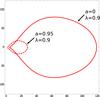 |
Fig. 1 Cross-section of the torus surface for a fixed angular momentum λ = 0.9 when varying the spin parameter from a = 0 (solid line) to a = 0.95 (dashed line). As the spin increases, the torus becomes smaller and its inner radius decreases. The axes are in units of the gravitational radius GM/c2. |
The electron number density distribution (Eq. (8)) is a rather non-trivial function of radius and angle. Figure 2 illustrates its profile in the equatorial plane as a function of radius for the same cases illustrated in Fig. 1, and compares it to the RIAF number density distribution. The RIAF distribution is taken from Broderick et al. (2011), Eq. (2): it is a simple power law with slope − 1.1. The torus model distribution is clearly not a power law, it is concentrated around the central radius of the torus, decreasing much more rapidly than the RIAF power law for bigger radii. As a consequence, the distant regions of the torus model will contribute less than the distant regions of the RIAF model. This point will be important later on.
3. Synchrotron radiation
In this section, we express the synchrotron emission and absorption coefficients for a directional magnetic field, and for either a thermal or non-thermal population of electrons. Radiative transfer for an angle-averaged magnetic field is simply obtained by angle-averaging the directional expressions.
3.1. Thermal directional synchrotron radiation
Wardziński & Zdziarski (2000) show that for a mildly relativistic Maxwellian electron distribution, ![Mathematical equation: \begin{eqnarray} n_{\rm e}(\gamma)=\frac{n_{\rm e}}{\theta_{\rm e}}\frac{\gamma(\gamma^2 - 1)^{1/2}}{K_2(1/\theta_{\rm e})}\exp\left[-\frac{\gamma}{\theta_{\rm e}}\right], \end{eqnarray}](/articles/aa/full_html/2015/02/aa24306-14/aa24306-14-eq87.png) (14)where θe = kBT/ (mec2), me being the electron mass, γ = (1 − v2/c2)− 1/2 is the Lorenz factor and K2 is a modified Bessel function, the emission coefficient is
(14)where θe = kBT/ (mec2), me being the electron mass, γ = (1 − v2/c2)− 1/2 is the Lorenz factor and K2 is a modified Bessel function, the emission coefficient is ![Mathematical equation: \begin{eqnarray} j_\nu^{\mathrm{dir,th}}&=&\frac{\pi e^2}{2c}(\nu\nu_0)^{1/2}\mathcal X(\gamma_0) n_{\rm e}(\gamma_0)\left(1 +2\frac{\cot^2\vartheta}{\gamma_0^2}\right)\nonumber\\ &&\times\left[1 - \left(1 - \gamma_0^{-2}\right) \cos^2\vartheta\right]^{1/4}\mathcal Z(\vartheta,\gamma_0) \end{eqnarray}](/articles/aa/full_html/2015/02/aa24306-14/aa24306-14-eq92.png) (15)where ν0 ≡ eB/ (2πmec) is the cyclotron frequency. Then,
(15)where ν0 ≡ eB/ (2πmec) is the cyclotron frequency. Then, ![Mathematical equation: \begin{eqnarray} \gamma_0= \displaystyle{\left[1 + \frac{2\nu\theta_{\rm e}}{\nu_0} \left(1 + \frac{9 \nu\theta_{\rm e}\sin^2\vartheta}{2 \nu_0}\right)^{-\frac 1 3}\right]^{\frac 1 2}} & \quad\theta_{\rm e} \lesssim 0.08 \nonumber\\ \nonumber\\ \displaystyle{\left[1 + \left(\frac{4\nu\theta_{\rm e}}{3 \nu_0\sin\vartheta}\right)^{\frac 2 3}\right]^{\frac 1 2}} & \quad\theta_{\rm e} \gtrsim 0.08 \end{eqnarray}](/articles/aa/full_html/2015/02/aa24306-14/aa24306-14-eq94.png) (16)is the Lorenz factor of those thermal electrons that contribute most to the emission at ν, and
(16)is the Lorenz factor of those thermal electrons that contribute most to the emission at ν, and ![Mathematical equation: \begin{eqnarray} \mathcal X(\gamma)= \begin{cases} \displaystyle{\left[\frac{2\theta_{\rm e}(\gamma^2 - 1)}{\gamma(3 \gamma^2 - 1)}\right]^{1/2}}, & \quad\theta_{\rm e} \lesssim 0.08\\ \\ \displaystyle{\left(\frac{2\theta_{\rm e}}{3\gamma}\right)^{1/2}}, & \quad\theta_{\rm e} \gtrsim 0.08 \end{cases} \end{eqnarray}](/articles/aa/full_html/2015/02/aa24306-14/aa24306-14-eq96.png) (17)
(17)![Mathematical equation: \begin{eqnarray} t &\equiv& (\gamma^2 - 1)^{\frac 1 2}\sin\vartheta, \quad n\equiv \frac{\nu(1 + t^2)}{\nu_0\gamma},\nonumber\\ \mathcal Z(\vartheta,\gamma)&=&\left\{\frac{t\exp[(1 + t^2)^{-\frac 1 2}]}{1 + (1 + t^2)^{\frac 1 2}}\right\}^{2n}\cdot \end{eqnarray}](/articles/aa/full_html/2015/02/aa24306-14/aa24306-14-eq97.png) (18)The absorption coefficient is simply given by Kirchhoff’s law:
(18)The absorption coefficient is simply given by Kirchhoff’s law:  where Bν is the Planck blackbody function.
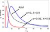 |
Fig. 2 Normalized distribution of the electron number density for the torus model with spin 0 and λ = 0.9 (solid blue) or spin 0.95 and λ = 0.9 (solid red). For comparison, the RIAF power-law distribution is plotted in dashed black (from Broderick et al. 2011). |
We note that our ray-tracing code allows to naturally take into account synchrotron self-absorption. The radiative transfer equation is simply solved along null geodesics until the torus becomes optically thick.
3.2. Non-thermal directional synchrotron radiation
Motivated by the RIAF model which is able to fit the whole radio (centimeter and millimeter) spectrum of Sgr A* using a population of non-thermal power-law electrons, we implemented such a population in our torus model.
We consider a population of electrons with a power-law energy spectrum 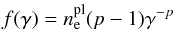 (19)where
  is the power-law electron number density. Following Özel et al. (2000) we assume that the energy of the non-thermal electrons is equal a small fraction δ of the energy of the thermal electrons. This leads to
  (20)where a(θe) is an order-unity function of temperature given by Özel et al. (2000), Eq. (6).
The power-law emission and absorption coefficients are then given by Petrosian & McTiernan (1983)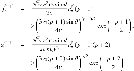 (21)We note here a typo in Özel et al. (2000) and Yuan et al. (2003): the frequency exponent of their absorption coefficient is not correct.
4. Torus model spectra
We use the open-source1 ray-tracing code GYOTO (Vincent et al. 2011) to compute images and spectra of the magnetized accretion torus. We have studied the impact of the models’ parameters on the observables in order to produce simulations that are in agreement with current constraints. Restricting ourselves to the centimeter and millimeter domains, we want our model to be able to reproduce the observed spectrum of Sgr A* (this section). The corresponding images should predict a correct size of the emitting zone which was constrained at 1σ to  as at 1.3 mm (intrinsic size) or
  as (scatter broadened) by Doeleman et al. (2008, next section).
In order to allow a direct comparison with the angle-averaged RIAF model, all torus model simulations are performed with angle-averaging unless otherwise stated.
4.1. Fitting the millimeter spectrum
The RIAF model is able to fit equally well any values of spin and inclination: these two parameters are not constrained by spectral data only (Broderick et al. 2011). We obtain the same behavior with our torus model: spin and inclination are not constrained from the millimeter spectral data only.
Our torus model is parameterized by a set of 7 parameters listed in Table 1. Here, we have always kept constant the plasma β parameter, to β = 10, as well as the polytropic index k = 5/3. For a given pair of spin and inclination, there are thus 3 parameters to fit: the torus constant angular momentum λ, its central temperature Tc and central density nc. We have performed a standard minimum χ2 analysis, minimizing the distance from model to data on a grid of parameters. We have been considering a grid of (λ,Tc,nc) with λ varying from 0.3 to 0.9, Tc from 7 × 10¹⁰ K to 3 × 10¹² K, and nc from 3 × 106 cm-3 to 107 cm-3. We have considered 30 × 30 × 10 values of (λ,Tc,nc) within these boundaries. We have investigated only extreme values of the spin parameter, a = 0 and a = 0.95, considering three values of inclination for both cases (i = 5°, i = 45°, i = 85°). Inclination is defined from the axis of rotation of the black hole to the line of sight: i = 5° means nearly face-on view.
Torus model parameters.
Table 2 gives the best-fit parameters for these configurations. It shows that all fits lead to  –0.4, thus to very good fits. Such low values of
  are obtained because of the large error of the 690 GHz data (see Fig. 3). This large error reflects the variability of the source rather than instrumental precision (see Marrone et al. 2006). All values of spin and inclination can thus be fitted with very good accuracy: the spectral millimeter data alone are not sufficient to constrain these parameters.
It is interesting to note that all best-fit physical values are rather close to each other, with rout ≈ 15, nc ≈ 5 × 106 cm-3, Tc ≈ 5 × 10¹¹ K. These values are in good agreement with other models of Sgr A* accretion flow, be they analytic or numeric (see e.g. Broderick & Loeb 2006; Mościbrodzka et al. 2009). A particularly striking point is the clear preference for very compact configurations, with the outer boundary of the torus being in all cases at 10–20 rg, translating to approximately 70 μas from the black hole position. This makes a big difference with respect to the RIAF model, for which the distribution of electrons is extended to regions far away from the black hole.
Torus model best-fit parameters for 2 extreme values of spin and a range of inclinations.
Figure 3 shows the 6 spectra associated to the best fits in Table 2. It is interesting to note that the thermal bump of the spectrum is always obtained at rather high frequency (between 1012 Hz and 5 × 10¹³ Hz). For completeness, Fig. 3 also shows the near-infrared upper limits: it is likely that some spin/inclination configuration might be excluded when fitting from radio to infrared data. However, here, the fit is only done on millimeter data, which means on the data points in Fig. 3 with frequency between ≈ 1011 Hz and 1012 Hz. The infrared upper limits are not taken into account in the fitting procedure.
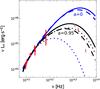 |
Fig. 3 Best-fitting spectra obtained for the parameters listed in Table 2. Blue curves are for spin 0, black for spin 0.95. Solid line is for i = 5°, dashed for i = 45°, and dotted for i = 85°. Note that the fitting is done only on the millimeter error bars. The infrared upper limits are given for completeness, but are not taken into account in the fit. |
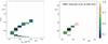 |
Fig. 4
|
4.2. Robustness of the fit results
We have analyzed in more detail the distribution of χ2 for the two cases in Table 2 corresponding to i = 85°. This choice was dictated by the fact that higher inclination is favored by the imaging constraints (see next section).
The first important result is that the size of the torus is indeed firmly constrained to values of rout ≲ 20 rg. At spin 0, all are above 1 for λ> 0.63, and all 0.5 ≤ λ ≤ 0.63 lead to spectra distant by more than 1σ from the 690 GHz data, which has a very large error bar due to the source variability. We conclude that we can safely constrain the angular momentum to λ< 0.5, equivalent to rout< 20. We obtain a comparable constraint from the a = 0.95 fit. The torus model is thus imposing a compact configuration.
Figure 4 shows the 2D distribution in the (nc,Tc) plane for the best-fitting value λ = 0.33 at spin 0 and inclination 85°. From the left panel, the central density is rather well constrained (up to a factor of 2), but the central temperature is allowed to vary by a factor of ≈10, always giving  . This freedom is only due to the large error bar at 690 GHz. The right panel of Fig. 4 shows the same distribution, but this error has been reduced by a factor of 3. The central temperature is immediately much more constrained. However, the best-fit value of Tc with a reduced error bar at 690 GHz differs from its counterpart with the unmodified error bar (while the central density remains unchanged). The central temperature changes from Tc = 2.3 × 10¹¹ K to Tc = 5.5 × 10¹¹ K. A very similar analysis could be made with spin 0.95 fit.
We conclude from this analysis that the fit results presented in Table 2 are robust as far as the angular momentum (or torus outer radius) and central density are concerned. The central temperature is less robust due to the large error bar at 690 GHz.
4.3. Impact of magnetic field geometry on the millimeter spectrum
One of our interest in this article is to investigate possible observable differences due to the magnetic field geometry. Figure 5 shows one of the best-fit spectra (a = 0.95, i = 85°), obtained for an angle-averaged configuration, together with the best-fit spectrum associated to a directional magnetic field. This directional best fit is found for the parameters λ = 0.85,nc = 6.3 × 106 cm-3,Tc = 3.6 × 10¹¹ K. The small difference between these directional parameters and their angle-averaged counterparts is mainly due to the difference in the relation between magnetic pressure and magnetic field magnitude (see Eqs. (9) and (13)).
The difference between the best-fit spectra is weak and it is not very surprising to conclude that spectral data will not be helpfull to constrain the magnetic field geometry.
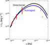 |
Fig. 5 Comparison of the best-fit a = 0.95, i = 85° spectra for an angle-averaged magnetic field (blue) and a directional toroidal magnetic field (black). Spectral data are not enough to put constraints on the magnetic field geometry. The infrared upper limits are given for completeness, but are not taken into account in the fit. |
4.4. No fit for the centimeter part of the spectrum
So far, we have been focused only on the millimeter part of Sgr A* spectrum, which is likely to be accounted for by thermal synchrotron. Lower radio frequencies are not fitted by a pure thermal population as the low-frequency slope of the thermal spectrum is too hard to fit the data. The RIAF model is able to fit this centimeter part of the spectrum by invoking a small proportion of non-thermal, power-law electrons (Özel et al. 2000). We have thus considered such a population in our model and tried to fit for the centimeter data.
Figure 6 shows the complete radio (centimeter to millimeter) spectrum associated to a = 0 and i = 5°, for both the torus model and the RIAF model. We have modeled a RIAF following Broderick et al. (2011). We consider a power-law distribution for electron density and temperature, following Eqs. (2) and (3) of Broderick et al. (2011). The non-thermal population is then constructed following the recipe given in Sect. 3.2. Figure 6 clearly shows that the RIAF model perfectly fits the whole radio spectrum, while the torus model is not able to reproduce the correct centimeter slope.
This difference between the two models is due to the very different electron distribution functions. It is well known that the νFν slope of power-law synchrotron equals 7/2. However, for an extended distribution of electrons, different parts of the accretion flow will emit different spectra, and the averaging of these spectra can end up in a much shallower slope. This is a well known effect in jets, and the same behavior is found in the RIAF model. However, the torus model electron distribution being much more compact, such an averaging is not obtained. We have checked that even for very big tori, the non-thermal spectrum slope is still too hard: indeed, as illustrated in Fig. 2, even for an extended torus, the electron distribution is clearly peaked towards small distances. We have also checked that decreasing the outer radius of the RIAF model leads to worse fits. For instance, in the simulation used in Fig. 6, the outer radius of the RIAF is at rout = 300 rg. Decreasing this value to rout = 100 rg leads to a very bad fit, the centimeter spectrum being too low (just as in the torus model), while the millimeter data are still perfectly fit.
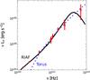 |
Fig. 6 Comparison of the best-fitting a = 0, i = 5° spectra as predicted by the RIAF model (solid black) and the torus model (dotted blue). A non-thermal power-law population of electrons is taken into account. The torus model is not able to fit the slope of the centimeter data because of the compact distribution of electrons, very different from the extended distribution of the RIAF model. |
We conclude that the torus model is still unable to fit the centimeter spectrum of Sgr A*. Another possibility to fit the centimeter data is to introduce a jet (Falcke & Markoff 2000). It is well known that Polish doughnuts, the base model of the torus model, can naturally funnel jets (Abramowicz et al. 1978). We plan in the future to investigate whether a torus+jet analytic model will be able to fit the whole radio specrum. The recent numeric study of such a configuration by Mościbrodzka & Falcke (2013) allows to be rather confident. In this perspective, the recent searches for a putative jet at the Galactic center are particularly meaningful (Yusef-Zadeh et al. 2012; Li et al. 2013).
To conclude this section, we highlight that our main result as far as spectral data are concerned is to demonstrate that the torus model is able to fit with perfect accuracy the millimeter spectrum of Sgr A*, and in particular the future EHT band. However, much work remains to be done in order to develop a complete synchrotron torus model of Sgr A*, from centimeter to near-infrared wavelengths. Even though our model cannot yet be considered self-consistent, we will investigate in the next section the image properties of the torus model at 1.3 mm. At this wavelength, the thermal synchrotron dominates, so we believe that our purely thermal model will give realistic predictions. We have checked that a pure thermal and a mixed thermal power-law image for the RIAF model are very similar at 1.3 mm.
5. Torus model images
5.1. 1.3 mm images for best-fit spectral models
Images of the best-fit models listed in Table 2 are readily computed at 1.3 mm, a wavelength at which a stringent limit on the size of the emitting region was imposed by Doeleman et al. (2008) at  as (1σ, scatter broadened). We need to model the smearing effect due to scattering by interstellar electrons. Following Mościbrodzka & Falcke (2013) we use a Gaussian profile with FWHM 1.309 λ2 (Falcke et al. 2000; Bower et al. 2006). At 1.3 mm this boils down to smearing the image with a Gaussian of FWHM ≈ 20 μas, already altering the image quite a lot.
Figure 7 shows the 1.3 mm images corresponding to the best-fit parameters of Table 2. Only the two higher values of inclination were considered as the size limit imposed by VLBI measurements favor higher inclination (Broderick et al. 2011). These images compare the size constraint of Doeleman et al. (2008) to the size of the region emitting 50% of the total flux. The figures show that constraints on the inclination parameter are at hand: at low spin, the i = 45° case is clearly excluded, and marginally acceptable for high spin. At i = 85°, the whole spin range will give a perfect fit to the size constraint.
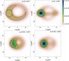 |
Fig. 7 Images (maps of specific intensity) at 1.3 mm of the best-fit models of Table 2. The dotted circle show the 1σ confidence domain from Doeleman et al. (2008). The thin solid curve encompass the region containing 50% of the total flux. The color bar is common to all panels, and graduated in cgs units (erg s-1 cm2 str-1 Hz-1). |
A complete study of the parameter space, fitting for the size of the emitting region for a grid of spins and inclinations, goes beyond the scope of the current article. It will be done in the future, once our model will have been made self consistent over the whole radio to infrared domain. The results presented here still support the torus model as they show that the size predicted in high-inclination configuration fits well the VLBI size constraint at 1.3 mm.
5.2. Impact of magnetic field geometry on the image
Figure 8 shows the comparison of the 1.3 mm images associated to the best-fit spectral model at a = 0.95,i = 85°, for the angle-averaged and directional models. It shows that the difference in the image is very weak, in the same way as for the spectral data. It is thus very unlikely that a constraint on the magnetic field geometry will be available by means of spectral and imaging data. The most natural way to get access to this information is to study the polarization properties of the radiation (see e.g. Zamaninasab et al. 2010).
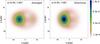 |
Fig. 8 Comparison of the best-fitting a = 0.95, i = 85° images at 1.3 mm for an angle-averaged magnetic field (left) and a directional toroidal magnetic field (right). |
6. Conclusion and perspectives
We have constructed a millimeter-wavelength synchrotron radiative model for Sgr A* based on the fully general relativistic, analytical magnetized torus model of Komissarov (2006). We have considered the original model with a toroidal magnetic field, as well as an angle-averaged, chaotic-magnetic-field configuration. We show that such a model is able to account for the observable spectral constraints in the millimeter domain. However, the torus model is not yet able of reproducing the centimeter data. Constraints on the emitting region size at 1.3 mm by Doeleman et al. (2008) are satisfied by the torus model provided inclination is high enough. We also show that the magnetic field geometry (chaotic or toroidal) cannot be constrained by spectral and imaging data. This work shows that the torus model is a serious candidate to account for the properties of Sgr A* close environment in the millimeter domain, which in particular encompasses the EHT observation band.
Our torus model is the third analytic model proposed to account for Sgr A* properties. The jet model (Falcke & Markoff 2000) and the RIAF model (Narayan et al. 1995; Özel et al. 2000; Yuan et al. 2003; Broderick et al. 2011) are alternatives. We have compared in this article the spectral predictions of the torus and RIAF models. This comparison shows that the RIAF model is able to account for the centimeter spectral data of Sgr A* because of its extended distribution of non-thermal electrons. As the torus model is firmly constrained to be compact (within ≈15 rg from the black hole), it cannot produce the same spectrum. Our goal is to develop in the near future a torus+jet model that would be able to account for both spectral and imaging constraints over the radio band.
The development of such a self-consistent analytic model over the full synchrotron band is interesting in the perspective of the future EHT data. Such an analytic model allows very fast computations as opposed to GRMHD simulations. For example, one spectrum or one image at a relatively low resolution, sufficient to fit the data, requires a few minutes of computation on a standard laptop for our model. This allows us to investigate large domains of physical parameters, which is not doable with GRMHD simulations because of the computational time limitation. In this perspective, we believe that the torus model for Sgr A* as developed in this work will be of interest for the future data analysis linked with the EHT project. In particular, this model may be a suitable test bed for investigating the observational counterparts of compact objects alternative to the Kerr black hole.
Freely available at the URL http://gyoto.obspm.fr
Acknowledgments
The authors are particularly grateful to the referee, Heino Falcke, for his careful reading of their first manuscript and his very accurate and relevant comments that allowed to greatly improve the quality of this paper. F.H.V. acknowledges interesting discussions with Monika Mościbrodzka at the first Black Hole Cam workshop in Effelsberg. This work was supported by five Polish NCN grants: 2011/01/B/ST9/05439, 2012/04/M/ST9/00780, 2013/08/A/ST9/00795, 2013/09/B/ST9/00060, and 2013/10/M/ST9/00729, together with the European “Synergy” grant CZ.1.07/2.3.00/20.0071 aimed to support international collaboration at the Institute of Physics of the Silesian University in Opava. This work was conducted within the scope of the HECOLS International Associated Laboratory, supported in part by the Polish NCN grant DEC-2013/08/M/ST9/00664. Computing was partly done using Division Informatique de l’Observatoire (DIO) HPC facilities from Observatoire de Paris (http://dio.obspm.fr/Calcul/).
References
- Abramowicz, M., Jaroszynski, M., & Sikora, M. 1978, A&A, 63, 221 [NASA ADS] [Google Scholar]
- Balick, B., & Brown, R. L. 1974, ApJ, 194, 265 [NASA ADS] [CrossRef] [Google Scholar]
- Bower, G. C., Goss, W. M., Falcke, H., Backer, D. C., & Lithwick, Y. 2006, ApJ, 648, L127 [NASA ADS] [CrossRef] [Google Scholar]
- Broderick, A. E., & Loeb, A. 2006, ApJ, 636, L109 [NASA ADS] [CrossRef] [Google Scholar]
- Broderick, A. E., Fish, V. L., Doeleman, S. S., & Loeb, A. 2011, ApJ, 735, 110 [NASA ADS] [CrossRef] [Google Scholar]
- Broderick, A. E., Johannsen, T., Loeb, A., & Psaltis, D. 2014, ApJ, 784, 7 [NASA ADS] [CrossRef] [Google Scholar]
- Chan, C.-k., Liu, S., Fryer, C. L., et al. 2009, ApJ, 701, 521 [NASA ADS] [CrossRef] [Google Scholar]
- Dexter, J., Agol, E., Fragile, P. C., & McKinney, J. C. 2010, ApJ, 717, 1092 [NASA ADS] [CrossRef] [Google Scholar]
- Doeleman, S., Agol, E., Backer, D., et al. 2009, Astronomy, 2010, 68 [NASA ADS] [Google Scholar]
- Doeleman, S. S., Weintroub, J., Rogers, A. E. E., et al. 2008, Nature, 455, 78 [NASA ADS] [CrossRef] [PubMed] [Google Scholar]
- Falcke, H., & Markoff, S. 2000, A&A, 362, 113 [NASA ADS] [Google Scholar]
- Falcke, H., Melia, F., & Agol, E. 2000, ApJ, 528, L13 [NASA ADS] [CrossRef] [PubMed] [Google Scholar]
- Genzel, R., Eisenhauer, F., & Gillessen, S. 2010, Rev. Mod. Phys., 82, 3121 [NASA ADS] [CrossRef] [Google Scholar]
- Ghez, A. M., Salim, S., Weinberg, N. N., et al. 2008, ApJ, 689, 1044 [NASA ADS] [CrossRef] [Google Scholar]
- Gillessen, S., Eisenhauer, F., Fritz, T. K., et al. 2009a, ApJ, 707, L114 [NASA ADS] [CrossRef] [Google Scholar]
- Gillessen, S., Eisenhauer, F., Trippe, S., et al. 2009b, ApJ, 692, 1075 [NASA ADS] [CrossRef] [Google Scholar]
- Goldston, J. E., Quataert, E., & Igumenshchev, I. V. 2005, ApJ, 621, 785 [NASA ADS] [CrossRef] [Google Scholar]
- Komissarov, S. S. 2006, MNRAS, 368, 993 [NASA ADS] [CrossRef] [Google Scholar]
- Leahy, J. P. 1991, in Beams and jets in astrophysics, ed. P. A. Hughes (Cambridge: Cambridge University Press) [Google Scholar]
- Li, Z., Morris, M. R., & Baganoff, F. K. 2013, ApJ, 779, 154 [NASA ADS] [CrossRef] [Google Scholar]
- Marrone, D. P., Moran, J. M., Zhao, J.-H., & Rao, R. 2006, J. Phys. Conf. Ser., 54, 354 [Google Scholar]
- McKinney, J. C., Tchekhovskoy, A., Sadowski, A., & Narayan, R. 2014, MNRAS, 441, 3177 [NASA ADS] [CrossRef] [Google Scholar]
- Mościbrodzka, M., & Falcke, H. 2013, A&A, 559, L3 [NASA ADS] [CrossRef] [EDP Sciences] [Google Scholar]
- Mościbrodzka, M., Gammie, C. F., Dolence, J. C., Shiokawa, H., & Leung, P. K. 2009, ApJ, 706, 497 [NASA ADS] [CrossRef] [Google Scholar]
- Narayan, R., & Yi, I. 1995, ApJ, 452, 710 [NASA ADS] [CrossRef] [Google Scholar]
- Narayan, R., Yi, I., & Mahadevan, R. 1995, Nature, 374, 623 [NASA ADS] [CrossRef] [Google Scholar]
- Noble, S. C., Leung, P. K., Gammie, C. F., & Book, L. G. 2007, Class. Quant. Grav., 24, 259 [Google Scholar]
- Özel, F., Psaltis, D., & Narayan, R. 2000, ApJ, 541, 234 [NASA ADS] [CrossRef] [Google Scholar]
- Petrosian, V., & McTiernan, J. M. 1983, Phys. Fluids, 3023, 26 [Google Scholar]
- Shcherbakov, R. V., Penna, R. F., & McKinney, J. C. 2012, ApJ, 755, 133 [NASA ADS] [CrossRef] [Google Scholar]
- Straub, O., Vincent, F. H., Abramowicz, M. A., Gourgoulhon, E., & Paumard, T. 2012, A&A, 543, A83 [NASA ADS] [CrossRef] [EDP Sciences] [Google Scholar]
- Vincent, F. H., Paumard, T., Gourgoulhon, E., & Perrin, G. 2011, Class. Quant. Grav., 28, 225011 [NASA ADS] [CrossRef] [Google Scholar]
- Wardziński, G., & Zdziarski, A. A. 2000, MNRAS, 314, 183 [NASA ADS] [CrossRef] [Google Scholar]
- Yuan, F., & Narayan, R. 2014, ARA&A, 52, 529 [NASA ADS] [CrossRef] [Google Scholar]
- Yuan, F., Quataert, E., & Narayan, R. 2003, ApJ, 598, 301 [NASA ADS] [CrossRef] [Google Scholar]
- Yusef-Zadeh, F., Arendt, R., Bushouse, H., et al. 2012, ApJ, 758, L11 [NASA ADS] [CrossRef] [Google Scholar]
- Zamaninasab, M., Eckart, A., Witzel, G., et al. 2010, A&A, 510, A3 [NASA ADS] [CrossRef] [EDP Sciences] [Google Scholar]
All Tables
Torus model best-fit parameters for 2 extreme values of spin and a range of inclinations.
All Figures
|
Fig. 1 Cross-section of the torus surface for a fixed angular momentum λ = 0.9 when varying the spin parameter from a = 0 (solid line) to a = 0.95 (dashed line). As the spin increases, the torus becomes smaller and its inner radius decreases. The axes are in units of the gravitational radius GM/c2. |
| In the text | |
|
Fig. 2 Normalized distribution of the electron number density for the torus model with spin 0 and λ = 0.9 (solid blue) or spin 0.95 and λ = 0.9 (solid red). For comparison, the RIAF power-law distribution is plotted in dashed black (from Broderick et al. 2011). |
| In the text | |
|
Fig. 3 Best-fitting spectra obtained for the parameters listed in Table 2. Blue curves are for spin 0, black for spin 0.95. Solid line is for i = 5°, dashed for i = 45°, and dotted for i = 85°. Note that the fitting is done only on the millimeter error bars. The infrared upper limits are given for completeness, but are not taken into account in the fit. |
| In the text | |
|
Fig. 4
|
| In the text | |
|
Fig. 5 Comparison of the best-fit a = 0.95, i = 85° spectra for an angle-averaged magnetic field (blue) and a directional toroidal magnetic field (black). Spectral data are not enough to put constraints on the magnetic field geometry. The infrared upper limits are given for completeness, but are not taken into account in the fit. |
| In the text | |
|
Fig. 6 Comparison of the best-fitting a = 0, i = 5° spectra as predicted by the RIAF model (solid black) and the torus model (dotted blue). A non-thermal power-law population of electrons is taken into account. The torus model is not able to fit the slope of the centimeter data because of the compact distribution of electrons, very different from the extended distribution of the RIAF model. |
| In the text | |
|
Fig. 7 Images (maps of specific intensity) at 1.3 mm of the best-fit models of Table 2. The dotted circle show the 1σ confidence domain from Doeleman et al. (2008). The thin solid curve encompass the region containing 50% of the total flux. The color bar is common to all panels, and graduated in cgs units (erg s-1 cm2 str-1 Hz-1). |
| In the text | |
|
Fig. 8 Comparison of the best-fitting a = 0.95, i = 85° images at 1.3 mm for an angle-averaged magnetic field (left) and a directional toroidal magnetic field (right). |
| In the text | |
Current usage metrics show cumulative count of Article Views (full-text article views including HTML views, PDF and ePub downloads, according to the available data) and Abstracts Views on Vision4Press platform.
Data correspond to usage on the plateform after 2015. The current usage metrics is available 48-96 hours after online publication and is updated daily on week days.
Initial download of the metrics may take a while.