| Issue |
A&A
Volume 570, October 2014
|
|
|---|---|---|
| Article Number | A94 | |
| Number of page(s) | 8 | |
| Section | Cosmology (including clusters of galaxies) | |
| DOI | https://doi.org/10.1051/0004-6361/201424179 | |
| Published online | 27 October 2014 | |
The Komatsu Spergel Wandelt estimator for oscillations in the cosmic microwave background bispectrum
1
Sorbonne Universités, UPMC Univ. Paris 06, UMR 7095, Institut
d’Astrophysique de Paris,
75014
Paris,
France
e-mail:
munchmey@iap.fr
2
CNRS, UMR 7095, Institut d’Astrophysique de Paris,
75014
Paris,
France
3
Lagrange Institute (ILP) 98bis boulevard Arago,
75014
Paris,
France
4
Department of Physics, University of Illinois at
Urbana-Champaign, Urbana, IL
61801,
USA
5
Department of Astronomy, University of Illinois at
Urbana-Champaign, Urbana, IL
61801,
USA
6
Paris Centre for Cosmological Physics and Laboratoire
AstroParticule et Cosmologie, Université Paris 7-Denis Diderot,
75205
Paris Cedex 13,
France
7
African Institute for Mathematical Sciences,
7945
Muizenberg, South
Africa
Received:
9
May
2014
Accepted:
1
August
2014
Oscillating shapes of the primordial bispectrum are present in many inflationary models. The Planck experiment has recently published measurements of oscillating shapes, which were, however, limited to the efficient frequency range of the used analysis method. Here, we study the Komatsu Spergel Wandelt (KSW) estimator for oscillations in the cosmic microwave background bispectrum, that examines arbitrary oscillation frequencies for separable oscillating bispectrum shapes. We study the precision with which amplitude, phase, and frequency can be determined with our estimator. An examination of the three-point function in real space gives further insight into the estimator.
Key words: cosmic background radiation / inflation / early Universe / cosmology: observations
© ESO, 2014
1. Introduction
The cosmic microwave background (CMB) provides the most direct experimental access to the statistics of the primordial curvature perturbations. In standard single-field, slow roll inflation, these perturbations are Gaussian to a very good approximation (Maldacena 2003). However, more complicated models of inflation often predict detectable amounts of non-Gaussianities of various shapes. In particular, the primordial bispectrum B(k1,k2,k3) arising from the three-point correlations of the curvature field ⟨ΦΦΦ⟩ is a sensitive probe to discriminate among models of inflation (see e.g. the reviews Liguori et al. 2010; Komatsu 2010; Yadav & Wandelt 2010). High precision measurements of the CMB recently provided by the Planck experiment (Planck Collaboration XXIV 2014) have been consistent with Gaussianity and set stronger limits on primordial non-Gaussianities. However, the availability of such limits depend on the specific shape of the bispectra under consideration.
A class of bispectra that has attracted attention in recent years are oscillating shapes. Such bispectrum oscillations can arise in a variety of theoretical models. The authors of Chen et al. (2008) calculated the primordial bispectrum in the presence of features in the inflaton potential of standard single field inflation. They provided two analytical bispectrum shapes that approximate their results. The feature model oscillates linearly with the scale and is induced by sharp features in the inflaton potential. The resonance model includes oscillations with the logarithm of the scale and is induced by periodic features in the inflaton potential. More recently, the authors of Bartolo et al. (2010) used the effective field theory of inflation to examine the influence of sharp features in the inflaton potential, which also provide oscillating bispectrum solutions. Periodical modulations of the inflaton potential appear, for example, in axion monodromy inflation models (Flauger et al. 2010; Flauger & Pajer 2011). Certain bispectrum shapes motivated by Non-Bunch-Davis vacua also include oscillations (e.g. Chen et al. 2007; Meerburg et al. 2009), as do cascade inflation models (Ashoorioon & Krause 2006). A transient reduction in the speed of sound also leads to oscillations (Achucarro et al. 2014b,a). Oscillations in the bispectrum are usually accompanied by oscillations in the primordial power spectrum. Recent searches for power spectrum oscillation were presented in Pahud et al. (2009); Peiris et al. (2013); Planck Collaboration XXII (2014); Easther & Flauger (2014); Meerburg et al. (2014); Meerburg & Spergel (2014), but no statistically significant result has been found. Combining power spectrum and bispectrum measurements can improve the sensitivity.
In the present work, we focus on the feature model shape, since it is simple and approximates some more complicated oscillating shapes. In particular, the feature model has the important property of separability. The Planck paper on non-Gaussianities (Planck Collaboration XXIV 2014) already included a targeted search for the feature and resonant shapes with the modal expansion method. In this methodology, the bispectrum under consideration is expanded into a basis of separable shapes (Fergusson et al. 2010), which allows an efficient numerical estimation by the Komatsu Spergel Wandelt (KSW) estimator (Komatsu et al. 2005). However, the separable basis functions used by Planck did not allow to represent high frequency oscillations, limiting the frequency range, which could be searched for oscillations. The situation can be improved by using a set of oscillating basis functions for the modal expansion (Meerburg 2010). In this work, we follow a more direct approach by writing the feature model bispectrum in separable form, which makes it possible to search for oscillations of arbitrary frequency, which are only limited by the resolution of the maps. The gain in computational time with respect to the modal expansion is of the order of the number of modes that would be necessary to approximate the shape. We study the properties of the estimator in detail, including the precision with which phase and frequency of the oscillation can be determined. We also give an illuminating interpretation of the KSW estimator for oscillations in position space.
2. Oscillations in the primordial bispectrum
2.1. Bispectrum shape and experimental constraints
The general translation and rotation invariant primordial bispectrum of the curvature
potential Φ can be written as
 (1)where the
bispectrum BΦ is a function of the magnitude of the
wave numbers ki and
fNL is the amplitude of the bispectrum.
The feature model bispectrum that we are primarily interested in is
(1)where the
bispectrum BΦ is a function of the magnitude of the
wave numbers ki and
fNL is the amplitude of the bispectrum.
The feature model bispectrum that we are primarily interested in is  (2)It oscillates
linearly with the mean,
(2)It oscillates
linearly with the mean,  , of the wave numbers. Here
ΔΦ is the
primordial power spectrum amplitude and the 1
/k6 factor compensates
for the phase space factor. The bispectrum is parametrised by the amplitude
fNL by the oscillation scale
kc and by the phase φ. The oscillation scale
kc implies an efficient multipole
periodicity of lc ≃
kc[τ −
τrec], where τ −
τrec is the conformal distance to
recombination.
, of the wave numbers. Here
ΔΦ is the
primordial power spectrum amplitude and the 1
/k6 factor compensates
for the phase space factor. The bispectrum is parametrised by the amplitude
fNL by the oscillation scale
kc and by the phase φ. The oscillation scale
kc implies an efficient multipole
periodicity of lc ≃
kc[τ −
τrec], where τ −
τrec is the conformal distance to
recombination.
Planck has searched for the feature bispectrum shape for sample frequencies in the range 0.01 <kc< 0.1 at four different phases φ = 0,π/ 4,π/ 2,3π/ 4Planck Collaboration XXIV (2014). Here, kc = 0.01 corresponds to an effective multipole periodicity lc = 140. The best fit model has kc = 0.0185 (lc = 260) and phase Φ = 0 with a significance of 3σ. This may correspond to weak hints for oscillation in the full bispectrum reconstruction, which were found for l< 500. However, the statistical significance becomes much lower when one takes the number of statistically uncorrelated feature models into account that were searched. We note that the range of the oscillation frequency was constrained because of the limitations of the analysis method. With the present work, we target the unexplored range kc< 0.01 in particular.
2.2. Separability
For convenience, we rewrite the feature model (2) as a sum of sine and cosine contributions as ![\begin{equation} \label{eq_oscispectrum3} B^{\mathrm{feat}}_\Phi(k_1,k_2,k_3) = \frac{6 \Delta_\Phi^2}{(k_1k_2k_3)^2} \left[ f_1 \sin\left(\frac{2\pi K}{3 k_{\rm c}}\right) + f_2 \cos\left(\frac{2\pi K}{3 k_{\rm c}}\right) \right], \end{equation}](/articles/aa/full_html/2014/10/aa24179-14/aa24179-14-eq26.png) (3)where
(3)where
 and
and  . This can be
written in separated form as
. This can be
written in separated form as ![\begin{eqnarray} \label{eq_oscispectrum4} B^{\mathrm{feat}}_\Phi(k_1,k_2,k_3) &= &6 f_1 \big[ -X(k_1) X(k_2) X(k_3) + \big(X(k_1) Y(k_2) Y(k_3) \nonumber \\ &&+ \textrm{2 perm.}\big) \big] + 6 f_2 \big[ Y(k_1) Y(k_2) Y(k_3) \nonumber \\ &&- \big( X(k_1) X(k_2) Y(k_3) + \textrm{2 perm.}\big) \big], \end{eqnarray}](/articles/aa/full_html/2014/10/aa24179-14/aa24179-14-eq29.png) (4)where
we have defined
(4)where
we have defined  (5)This separability
property allows efficient computation and estimation of the bispectrum. One may also
include an exponential decay factor of the form
(5)This separability
property allows efficient computation and estimation of the bispectrum. One may also
include an exponential decay factor of the form  ,
while retaining separability with identical formulas up to trivial replacements.
,
while retaining separability with identical formulas up to trivial replacements.
3. Oscillations in the CMB bispectrum
From the separable expression (4) for the
primordial bispectrum, one can calculate the CMB bispectrum with the standard line-of-sight
integration method Seljak & Zaldarriaga
(1996). The reduced bispectrum is then ![\begin{eqnarray} \label{eq_reducedbispectrum1} b_{l_1l_2l_3} &= &6 f_1 \int {\rm d}r~r^2~ \big[-X_{l_1}(r) X_{l_2}(r) X_{l_3}(r) + ( X_{l_1}(r) Y_{l_2}(r) Y_{l_3}(r) \nonumber\\ &&+ \textrm{2 perm.}) \big] + 6 f_2 \int {\rm d}r~r^2~ \big[ Y_{l_1}(r) Y_{l_2}(r) Y_{l_3}(r) \nonumber\\ &&- (X_{l_1}(r) X_{l_2}(r) Y_{l_3}(r) + \textrm{2 perm.}) \big]. \end{eqnarray}](/articles/aa/full_html/2014/10/aa24179-14/aa24179-14-eq32.png) (6)where
we have defined the functions
(6)where
we have defined the functions 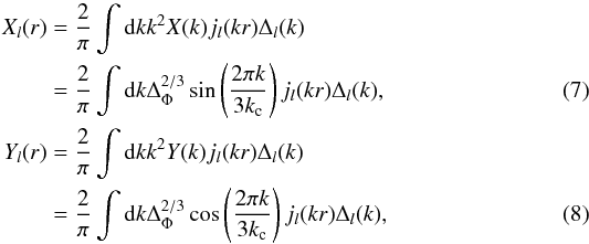 and
where jl are spherical Bessel
functions and Δl are the CMB transfer functions that we
evaluate numerically with CAMB Lewis et al. (2000).
We note that these functions depend on kc and have to be evaluated for each
oscillation frequency of interest. Both the transfer functions Δl(k) (in k space) and the Bessel
functions jl are highly
oscillatory integrals, which must be evaluated with sufficient sampling. Examples of the
X(r) and Y(r)
functions are given in Fig. 1.
and
where jl are spherical Bessel
functions and Δl are the CMB transfer functions that we
evaluate numerically with CAMB Lewis et al. (2000).
We note that these functions depend on kc and have to be evaluated for each
oscillation frequency of interest. Both the transfer functions Δl(k) (in k space) and the Bessel
functions jl are highly
oscillatory integrals, which must be evaluated with sufficient sampling. Examples of the
X(r) and Y(r)
functions are given in Fig. 1.
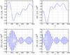 |
Fig. 1 Function X and Y of the feature model for kc = 0.01 (top) and kc = 0.001 (bottom) as a function of l for r = τ0 − τrec. X and Y have units of Mpc-1. |
To calculate the resulting CMB bispectrum, we perform the r integral in Eq. (6). We choose a quadrature of about 2000 points
in r with a
higher sampling in the range of recombination. The contribution of different values of
r is examined
in more detail in Sect. 6. To plot the bispectrum, it
is convenient to normalise by the constant bispectrum with natural k-6 scaling, as
proposed in Fergusson & Shellard (2009). The
constant primordial bispectrum is given by  (9)and its large angle
Sach-Wolfe CMB solution is Fergusson & Shellard
(2009)
(9)and its large angle
Sach-Wolfe CMB solution is Fergusson & Shellard
(2009)![\begin{eqnarray} \label{eq_blconstsw} b^{\rm const}_{l_1l_2l_3} &=& \left(\frac{1}{3}\right)^3 \frac{1}{(2l_1+1) (2l_2+1) (2l_3+1)} \nonumber\\ &&\quad \times \left[ \frac{1}{l_1 +l_2+l_3+3} + \frac{1}{l_1+l_2+l_3} \right]\cdot \end{eqnarray}](/articles/aa/full_html/2014/10/aa24179-14/aa24179-14-eq50.png) (10)In
Fig. 2, we show a simple 1-dimensional visualisation,
the equal l
bispectrum blll normalised by
(10)In
Fig. 2, we show a simple 1-dimensional visualisation,
the equal l
bispectrum blll normalised by
 for
different frequencies and phases of the feature model.
for
different frequencies and phases of the feature model.
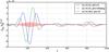 |
Fig. 2 Equal l reduced bispectrum normalised by the large angle solution of the constant bispectrum for feature models with different parameters. |
4. The KSW estimator for the oscillating bispectrum
4.1. KSW estimator
The optimal KSW estimator for a sum of bispectra bi in the presence of a
mask and non-uniform noise is (Komatsu et al. 2005;
Babich 2005; Komatsu 2010)  (11)with
 ![\begin{eqnarray} \label{eq_kswphase2} S_i &= &\frac{1}{6} \sum_{lm} G^{m_1m_2m_3}_{l_1l_2l_3} b^i_{l_1l_2l_3} \Big[ (C^{-1}a)_{l_1m_1} (C^{-1}a)_{l_2m_2} (C^{-1}a)_{l_3m_3} \nonumber\\ &&- 3 \left(C^{-1}\right)_{l_1m_1,l_2m_2} (C^{-1}a)_{l_3m_3} \Big] \end{eqnarray}](/articles/aa/full_html/2014/10/aa24179-14/aa24179-14-eq55.png) (12)and
with the Fisher matrix given by
(12)and
with the Fisher matrix given by  (13)In
the present case of an oscillation with a single scale kc, the
bispectrum is a sum b =
f1b1 +
f2b2 of sine
and cosine components, as given by Eq. (6).
(13)In
the present case of an oscillation with a single scale kc, the
bispectrum is a sum b =
f1b1 +
f2b2 of sine
and cosine components, as given by Eq. (6).
To numerically evaluate the KSW estimator terms Si we need the weighted
maps  (14)The
cubic KSW estimator, which is exact in the case of a full sky observation, is given in
terms of these maps by
(14)The
cubic KSW estimator, which is exact in the case of a full sky observation, is given in
terms of these maps by ![\begin{eqnarray} \label{eq_ksw2} S^{\rm cub}_1 &=& \! \int\! r^2 {\rm d}r \!\int\! {\rm d}\Omega \left[ -M^3_X(r,\hat{n}) +\left(3 M_X(r,\hat{n}) M_Y(r,\hat{n}) M_Y(r,\hat{n})\right) \right], \nonumber\\ S^{\rm cub}_2 &=& \!\int\! r^2 {\rm d}r \!\int \!{\rm d}\Omega \left[ M^3_Y(r,\hat{n}) -\left(3 M_X(r,\hat{n}) M_X(r,\hat{n}) M_Y(r,\hat{n})\right) \right]. \end{eqnarray}](/articles/aa/full_html/2014/10/aa24179-14/aa24179-14-eq60.png) (15)Partial
sky coverage can be taken into account by incorporating the linear term of the KSW
estimator, so that
(15)Partial
sky coverage can be taken into account by incorporating the linear term of the KSW
estimator, so that  with
with
![\begin{eqnarray} \label{eq_ksw3} S_1^{\rm lin} &= &-3\int r^2 {\rm d}r \int {\rm d}\Omega \bigl[- M_X(r,\hat{n}) \left< M^2_X(r,\hat{n}) \right> \nonumber\\ &&+ M_X(r,\hat{n}) \left< M^2_Y(r,\hat{n}) \right> + 2 M_Y(r,\hat{n}) \left< M_X(r,\hat{n}) M_Y(r,\hat{n}) \right> \bigr], \nonumber\\ S_2^{\rm lin}& = &-3\int r^2 {\rm d}r \int {\rm d}\Omega \bigl[ M_Y(r,\hat{n}) \left< M^2_Y(r,\hat{n}) \right> \nonumber\\ &&- M_Y(r,\hat{n}) \left< M^2_X(r,\hat{n}) \right> - 2 M_X(r,\hat{n}) \left< M_X(r,\hat{n}) M_Y(r,\hat{n}) \right>\bigr], \end{eqnarray}](/articles/aa/full_html/2014/10/aa24179-14/aa24179-14-eq62.png) (16)where
the expectation values have to be evaluated by Monte Carlo averaging over Gaussian
realisations drawn with the same beam, mask, and noise properties as expected in the data.
To make the KSW estimator optimal for a non-uniform sky coverage, it is necessary to
perform an inverse covariance weighting with the non-diagonal covariance matrix. This is a
computationally challenging problem (Smith et al.
2009; Elsner & Wandelt 2012). It
was noted in Planck Collaboration XXIV (2014) that
one can also achieve excellent results by assuming a diagonal covariance matrix
Ĉl =
Cl +
Nl, where
Nl assumes homogeneous
noise, and by using a diffusive inpainting on the masked areas. In this approximation, the
Fisher matrix scales proportionally to the visible fraction of the sky fsky.
(16)where
the expectation values have to be evaluated by Monte Carlo averaging over Gaussian
realisations drawn with the same beam, mask, and noise properties as expected in the data.
To make the KSW estimator optimal for a non-uniform sky coverage, it is necessary to
perform an inverse covariance weighting with the non-diagonal covariance matrix. This is a
computationally challenging problem (Smith et al.
2009; Elsner & Wandelt 2012). It
was noted in Planck Collaboration XXIV (2014) that
one can also achieve excellent results by assuming a diagonal covariance matrix
Ĉl =
Cl +
Nl, where
Nl assumes homogeneous
noise, and by using a diffusive inpainting on the masked areas. In this approximation, the
Fisher matrix scales proportionally to the visible fraction of the sky fsky.
For the remainder of this paper, we assume full sky coverage so that  (17)where
 .
.
From the inverse Fisher matrix (i.e. the covariance), one obtains the correlation between
the sine and cosine terms. For example, for l = 1000 and kc = 0.01, the
correlation matrix is 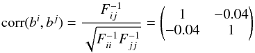 (18)which
shows a weak correlation as expected. From f1 and f2 of Eq. (6), we can calculate the amplitude and phase of
the oscillation. The variance of the quantities fNL and Φ can be calculated by error propagation
from f1 and f2. For example
(18)which
shows a weak correlation as expected. From f1 and f2 of Eq. (6), we can calculate the amplitude and phase of
the oscillation. The variance of the quantities fNL and Φ can be calculated by error propagation
from f1 and f2. For example
 (19)In the approximation of a
diagonal covariance matrix and σf1 =
σf2, this
gives σf =
σf1. In
this approximation the sensitivity on the phase depends on f as
(19)In the approximation of a
diagonal covariance matrix and σf1 =
σf2, this
gives σf =
σf1. In
this approximation the sensitivity on the phase depends on f as
 .
.
The Fisher matrix allows us to forecast the precision that can be obtained on the
bispectrum parameters f1,f2.
With the approximation that the f1,f2
covariance matrix is a multiple of the unit matrix, the Fisher forecast on f1,f2
equals the forecast on fNL. The precision on fNL is then
given by  .
For a noiseless full-sky experiment, the Fisher forecast for the feature model is shown in
Fig. 3 for a number of different oscillation
frequencies.
.
For a noiseless full-sky experiment, the Fisher forecast for the feature model is shown in
Fig. 3 for a number of different oscillation
frequencies.
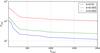 |
Fig. 3 Fisher forecast of σfNL for the feature model for different kc, assuming a noiseless full sky experiment. |
4.2. Estimating the frequency
The estimator described above explicitly estimates the amplitude fNL and phase
φ of the
oscillation for a fixed frequency kc. To estimate the oscillation
frequency kc, it is necessary to sample the
frequency space with the KSW estimator and search for peaks in the significance of the
estimated amplitude. We assume the primordial bispectrum to be given by a single
oscillation frequency and not a spectrum of contributions. We consider only the sine
component of the bispectrum first, meaning that the phase is φ = 0 (see below for the
generalisation to the phase). In this case, the estimator for a frequency ki is  (20)with
covariance (in the usual Gaussian approximation)
(20)with
covariance (in the usual Gaussian approximation)  The
Fisher matrix is given by Eq. (13), where
the index i
now goes over frequency sampling points. An example of the Fisher matrix Fij is shown in Fig.
4 (top). The corresponding correlation matrix is
The
Fisher matrix is given by Eq. (13), where
the index i
now goes over frequency sampling points. An example of the Fisher matrix Fij is shown in Fig.
4 (top). The corresponding correlation matrix is
 ,
shown in Fig. 4 (middle).
,
shown in Fig. 4 (middle).
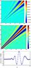 |
Fig. 4 Top: fisher matrix Fij for 100
logarithmically spaced frequencies between kc = 0.002
and kc =
0.01. Middle: corresponding correlation matrix
|

A one-dimensional slice of the correlation matrix is shown in Fig. 4 (bottom) for kc = 0.005. The plot shows strong anti-peaks to both sides of the maximum and several small secondary peaks. This is not an artefact of the chosen estimator, but the physical overlap of the CMB bispectra induced by different primordial oscillation frequencies. The frequency sampling must be at least sufficient to resolve the peak structure of this plot. However, the width of the central peak does not directly limit the precision σk with which the primordial frequency can be determined.
To evaluate the precision with which kc can be estimated, we note that the
correlation matrix is identical to the bispectrum correlator, 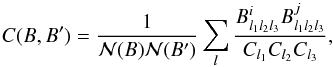 (23)which is the usual
measure to discriminate bispectra (see e.g. Fergusson
& Shellard 2009). It gives the estimated proportion of f that is recovered when
estimating a spectrum B′ when the true underlying spectrum is
B. If the
underlying bispectum is fkcBkc,
the expectation value of the estimated amplitude at a different frequency k is thus
(23)which is the usual
measure to discriminate bispectra (see e.g. Fergusson
& Shellard 2009). It gives the estimated proportion of f that is recovered when
estimating a spectrum B′ when the true underlying spectrum is
B. If the
underlying bispectum is fkcBkc,
the expectation value of the estimated amplitude at a different frequency k is thus
 ).
The variance at each data point is independent of the signal. Thus, the correlation matrix
approximates the estimates in the k range where the signal dominates the variance
(compare Fig. 4 with the estimation example in Fig.
6).
).
The variance at each data point is independent of the signal. Thus, the correlation matrix
approximates the estimates in the k range where the signal dominates the variance
(compare Fig. 4 with the estimation example in Fig.
6).
Knowing the means f(k) and the covariance matrix
Cov(k1,k2)
and using the property that each estimator  is Gaussian distributed, we can write the continuum likelihood for the estimated
amplitudes ,
if the true bispectrum is fkcBkc:
is Gaussian distributed, we can write the continuum likelihood for the estimated
amplitudes ,
if the true bispectrum is fkcBkc:
![\begin{eqnarray} \label{eq_kclikeli} -2 &&\ln ~\mathcal{L}(\hat{f}(k)|f_{k_{\rm c}},k_{\rm c}) = \ln|{\rm Cov}| \nonumber \\ &&+\left[ \int {\rm d}k_1 {\rm d}k_2 ~(\hat{f}(k_1) - \mu(k_1)) ~ {\rm Cov}^{-1}(k_1,k_2) ~ (\hat{f}(k_2) - \mu(k_2)) \right], \end{eqnarray}](/articles/aa/full_html/2014/10/aa24179-14/aa24179-14-eq100.png) (24)with
mean
(24)with
mean  (25)This likelihood could
be explored by Monte Carlo to find maximum likelihood estimates of fkc and
kc if a significant peak of
fNL is found in the spectrum. The Fisher
matrix to forecast optimal precision on the estimated parameters is
(25)This likelihood could
be explored by Monte Carlo to find maximum likelihood estimates of fkc and
kc if a significant peak of
fNL is found in the spectrum. The Fisher
matrix to forecast optimal precision on the estimated parameters is  (26)where θ ∈ {
fkc,kc
}. This can be integrated numerically for any given fiducial
parameters.
(26)where θ ∈ {
fkc,kc
}. This can be integrated numerically for any given fiducial
parameters.
In the above discussion, we assumed that the bispectrum only has a sine contribution. The
generalisation of Eq. (24) to a free phase
is  (27)with
the mean
(27)with
the mean  (28)The correlation
matrix can be split into terms of f1 and f2 for efficient
evaluation of the likelihood.
(28)The correlation
matrix can be split into terms of f1 and f2 for efficient
evaluation of the likelihood.
As we have seen, the estimation of the frequency requires to run a large number of estimators (around 100 to cover the frequency interval kc = 0.001 to kc = 0.01). For each of these estimators, it is necessary to calculate the linear term in Eq. (16) via a Monte Carlo averaging procedure over Gaussian map realisations with the same mask and noise properties as present in the experiment. Convergence of the linear term is usually achieved with 100 Monte Carlo realisations, although several hundreds can be used to improve accuracy. After the optimisation of the conformal distance integral, that is reviewed in Sect. 6, one can expect, with an angular resolution of lmax = 2000, a calculation time of about one day on a single cpu for a single frequency, including the Monte Carlo averaging. On a computation grid, one can thus easily cover the frequency range of interest.
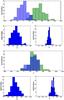 |
Fig. 5 Parameter estimation histograms for 100 maps with linear model non-Gaussianity with kc = 0.01 and lmax = 1000. The maps were created with fNL = 500 and φ = 0° (first two rows) and φ = 45° (rows three and four). Top: reconstructed f1 (green) and f2 (blue) amplitudes for φ = 0°. Second row: corresponding reconstructed amplitudes fNL and phases φ. Third and fourth row: same as above but with phase φ = 45°. |
5. Map making
To verify the implementation and unbiased nature of the estimator, it is useful to be able
to generate maps with the bispectrum signature of interest. The authors of Smith & Zaldarriaga (2011) introduced an
algorithm that generates maps for arbitrary bispectra in the weak non-Gaussian limit. A map
is constructed from a linear combination of a Gaussian and a non-Gaussian contribution as
 . The
straightforward implementation of the algorithm gives a non-Gaussian contribution of the
form
. The
straightforward implementation of the algorithm gives a non-Gaussian contribution of the
form ![\begin{eqnarray} \label{eq_map1} a^{\rm NL}_{lm} &= & f_1 \int r^2 {\rm d}r \Biggl[ - X_l(r) \int {\rm d}\Omega ~Y_{lm}^* M^2_X(r,\hat{n}) \nonumber\\ &&+\left( X_l(r) \int {\rm d}\Omega ~Y_{lm}^* M_Y(r,\hat{n}) M_Y(r,\hat{n}) + 2 \mathrm{perm.} \right) \Biggr] \nonumber\\ &&+ f_2 \int r^2 {\rm d}r \Biggl[ Y_l(r) \int {\rm d}\Omega ~Y_{lm}^* M^2_Y(r,\hat{n}) \nonumber\\ &&-\left(Y_l(r) \int {\rm d}\Omega ~Y_{lm}^* M_X(r,\hat{n}) M_X(r,\hat{n}) + 2 \mathrm{perm.} \right) \Biggr]. \end{eqnarray}](/articles/aa/full_html/2014/10/aa24179-14/aa24179-14-eq114.png) (29)It
is thus easy to create maps of arbitrary phase from the sine and cosine terms.
(29)It
is thus easy to create maps of arbitrary phase from the sine and cosine terms.
An example of two sets of 100 maps, created and then estimated with the algorithms presented here, is shown in Fig. 5. The means and variances in these histograms are compatible with their Fisher forecast. We note that the distribution of fNL is not Gaussian but follows a Rayleigh distribution, since fNL represents the magnitude of the vector of the two directional components f1 and f2.
An example of a frequency sweep can be found in Fig. 6 for the phase ϕ = 0°. It shows the secondary peaks that are expected from the correlation of different frequencies.
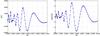 |
Fig. 6 Left: frequency sweep over a map with kc = 0.005 and fNL = 2000. Right: as left but in units of σfNL. |
6. Computational speed improvement by optimisation of the r-integral
Due to the large number of frequencies that have to be sampled with the corresponding estimator, the search for oscillations is computationally challenging. The time critical steps are the calculation of the Fisher matrix and the necessity of calculating a large number of r dependent KSW filtered maps. The latter problem becomes even more severe if one has to estimate many Monte Carlo generated maps for the calculation of the linear term. The situation can be improved by an analysis of the Fisher matrix, as shown in Smith & Zaldarriaga (2011).
For a separable shape, the Fisher matrix can also be expressed by a sum over contributions
of different r
sampling points that arise when numerically evaluating the bispectrum integral in Eq. (6). The total Fisher matrix is then given as a
sum  , where
Fij is the Fisher matrix
element between the sampling points i and j and Nfact is the number of sampling points.
The Fisher matrix elements are then given by
, where
Fij is the Fisher matrix
element between the sampling points i and j and Nfact is the number of sampling points.
The Fisher matrix elements are then given by  (30)We
now explicitly consider the sine term of the linear model (the cosine term is analogous),
where the contribution of a distance ri is given by
(30)We
now explicitly consider the sine term of the linear model (the cosine term is analogous),
where the contribution of a distance ri is given by
![\begin{eqnarray} \label{eq_fisher3} b^i_{l_1l_2l_3} &=& (\Delta r_i) r_i^2 \big[-X_{l_1}(r_i) X_{l_2}(r_i) X_{l_3}(r_i)\nonumber \\ &&\quad+ \left[ X_{l_1}(r_i) Y_{l_2}(r_i) Y_{l_3}(r_i) + \textrm{2 perm.}\right] \big]. \end{eqnarray}](/articles/aa/full_html/2014/10/aa24179-14/aa24179-14-eq123.png) (31)To
give an impression of the bispectrum contribution of different distances ri, we plot the diagonal
elements Fii in Fig. 7. The plots show the contribution of recombination
(r = 14 000
Mpc), reionisation (r ≃ 10
500 Mpc), and ISW (r> 5000 Mpc). As expected,
the dominant contribution comes from the time around recombination, and one can get a good
approximation to the integral by sampling only a window around recombination. This is
particularly useful to quickly scan a parameter space, in the present case the oscillation
frequency, kc.
(31)To
give an impression of the bispectrum contribution of different distances ri, we plot the diagonal
elements Fii in Fig. 7. The plots show the contribution of recombination
(r = 14 000
Mpc), reionisation (r ≃ 10
500 Mpc), and ISW (r> 5000 Mpc). As expected,
the dominant contribution comes from the time around recombination, and one can get a good
approximation to the integral by sampling only a window around recombination. This is
particularly useful to quickly scan a parameter space, in the present case the oscillation
frequency, kc.
In Smith & Zaldarriaga (2011), it was shown
that one can go further and optimise the r sampling points to find a quadrature with
surprisingly few sampling points that give an almost identical estimator. Their algorithm
constructs a new bispectrum B′ from the original bispectrum
B by choosing
a subsample of points and weighting them so that the Fisher distance between the two is
minimised:  (32)This means that bispectrum
values with a small signal-to-noise are allowed to be very different. Using this algorithm,
as an example, we obtain an approximate bispectrum B′ consisting of
30 sample points leading to a separability between B and B′ of
0.1σ assuming
kc =
0.01 and fNL = 1000.
(32)This means that bispectrum
values with a small signal-to-noise are allowed to be very different. Using this algorithm,
as an example, we obtain an approximate bispectrum B′ consisting of
30 sample points leading to a separability between B and B′ of
0.1σ assuming
kc =
0.01 and fNL = 1000.
The most computationally demanding task in the estimation pipeline remains the calculation
of the Fisher matrix in Eq. (30). It was
also shown in Smith & Zaldarriaga (2011) that
one can factorise this equation by inserting the integral representation of the Wigner
symbol  (33)The integral over
z can be
computed efficiently by Gauss Legendre integration. However, even with this expression, the
calculation of Fij needs many CPU
hours depending on the chosen initial quadrature point number. If one does not want to
calculate an optimised quadrature at every frequency points, but only wants to know the
normalisation F(kc) of the estimators,
one can calculate this normalisation on a much wider frequency spacing and interpolate in
between. This can be seen from the frequency dependent Fisher matrix in Fig. 4, where the diagonal elements vary slowly.
(33)The integral over
z can be
computed efficiently by Gauss Legendre integration. However, even with this expression, the
calculation of Fij needs many CPU
hours depending on the chosen initial quadrature point number. If one does not want to
calculate an optimised quadrature at every frequency points, but only wants to know the
normalisation F(kc) of the estimators,
one can calculate this normalisation on a much wider frequency spacing and interpolate in
between. This can be seen from the frequency dependent Fisher matrix in Fig. 4, where the diagonal elements vary slowly.
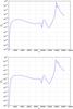 |
Fig. 7 Fii as a function of conformal distance ri. Top: kc = 0.01, bottom: kc = 0.005. |
7. A position space interpretation of the KSW estimator for oscillations
In Appendix A, we show that the three-point function of the feature model in position space
peaks for configurations  that lie on a circumcircle of radius sin(θ) = 1 /
(2k0η), where
that lie on a circumcircle of radius sin(θ) = 1 /
(2k0η), where
 in the convention of
Eq. (2). This suggests searching for
bispectrum oscillations in real space by convoluting the CMB map with a ring kernel of
varying radius.
in the convention of
Eq. (2). This suggests searching for
bispectrum oscillations in real space by convoluting the CMB map with a ring kernel of
varying radius.
For a radially symmetric kernel, the convolution can be done efficiently in harmonic space
as slm =
Klrlm,
where the kernel is given by the Legendre transformation,  (34)and K(z) is a
narrow window function in z =
cos(θ). The estimate ℰring(z) is given
by the sum over the pixels of the cube of the convoluted map,
(34)and K(z) is a
narrow window function in z =
cos(θ). The estimate ℰring(z) is given
by the sum over the pixels of the cube of the convoluted map, ![\begin{equation} \label{eq_ringestimate} \mathcal{E}^{\rm ring} (z_0) = \int {\rm d}\Omega \left[ \sum_{lm} K_l a_{lm} Y_{lm} \right]^3. \end{equation}](/articles/aa/full_html/2014/10/aa24179-14/aa24179-14-eq142.png) (35)Figure 8 shows an example of this estimator for a map that was
simulated with the algorithm of the preceding section. The plots show
(35)Figure 8 shows an example of this estimator for a map that was
simulated with the algorithm of the preceding section. The plots show
 , which means
that the estimate from the Gaussian map was subtracted. The red line shows the predicted
position of the maximum. We note that this maximum would be harder to locate in real data
where the Gaussian contribution cannot simply be subtracted.
, which means
that the estimate from the Gaussian map was subtracted. The red line shows the predicted
position of the maximum. We note that this maximum would be harder to locate in real data
where the Gaussian contribution cannot simply be subtracted.
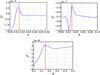 |
Fig. 8 Ring estimate |
It is interesting to compare the “intuitive” ring kernel K(θ) with
the KSW kernel that is known to give optimal results. The KSW estimator is of form,
![\begin{equation} \label{eq_kernel3} \mathcal{E}^{\rm KSW}(a) \propto \int r^2 {\rm d}r \int {\rm d}\Omega \left[ \sum_{lm} \frac{X_l a_{lm}}{C_l} Y_{lm} \right]^3 + ... . \end{equation}](/articles/aa/full_html/2014/10/aa24179-14/aa24179-14-eq147.png) (36)The largest contribution
to this integral comes from decoupling at rrec. We plot the KSW kernel function at
decoupling Xrec(θ) in Fig. 9. It shows the maximum at the expected position and has
roughly the expected window shape.
(36)The largest contribution
to this integral comes from decoupling at rrec. We plot the KSW kernel function at
decoupling Xrec(θ) in Fig. 9. It shows the maximum at the expected position and has
roughly the expected window shape.
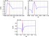 |
Fig. 9 KSW kernel X(θ) at decoupling radius rrec. Top left: kc = 0.01. Top right: kc = 0.005. Bottom: kc = 0.001. The red line is the predicted maximum of the kernel. |
8. Conclusion
In this paper, we have presented and extensively studied the KSW estimator for linear bispectrum oscillations. The main motivation for this approach is that the oscillating bispectrum shapes are difficult to represent with a modal expansion and, thus, have not yet been constrained at high oscillation frequency. We have provided the equations for estimation and map making and validated them with Monte Carlo simulations. Unlike many of the well know bispectum shapes, oscillations have two free parameters in addition to the common amplitude parameter fNL. We have developed the methodology to estimate and constrain the oscillation phase φ and the frequency kc. Our work will therefore allow one to explore a parameter space that was not previously accessible for a theoretically well-motivated bispectrum shape. Finally, we have found an interesting position space interpretation of the KSW estimator for oscillations, based on an approximate evaluation of the corresponding three-point function.
Acknowledgments
The authors acknowledge support from NSF Grant NSF AST 09-08693 ARRA. B.D.W. acknowledges funding from an ANR Chaire d’Excellence (ANR-10-CEXC-004-01), the UPMC Chaire Internationale in Theoretical Cosmology, and NSF grants AST-0908 902 and AST-0708849. This work made in the ILP LABEX (under reference ANR-10-LABX-63) was supported by French state funds managed by the ANR within the Investissements d’Avenir programme under reference ANR-11-IDEX-0004-02. M.M. acknowledges funding by Centre National d’Etudes Spatiales (CNES). The authors would like to thank Daan Meerburg for useful discussions and comments.
References
- Achucarro, A., Atal, V., Hu, B., Ortiz, P., & Torrado, J. 2014a, Phys. Rev. D, 90, 023511 [NASA ADS] [CrossRef] [Google Scholar]
- Achucarro, A., Atal, V., Ortiz, P., & Torrado, J. 2014b, Phys. Rev. D, 89, 103006 [NASA ADS] [CrossRef] [Google Scholar]
- Adshead, P., Dvorkin, C., Hu, W., & Lim, E. A. 2012, Phys. Rev. D, 85, 023531 [NASA ADS] [CrossRef] [Google Scholar]
- Ashoorioon, A., & Krause, A. 2006 [arXiv:hep-th/0607001] [Google Scholar]
- Babich, D. 2005, Phys. Rev. D, 72, 043003 [NASA ADS] [CrossRef] [Google Scholar]
- Bartolo, N., Fasiello, M., Matarrese, S., & Riotto, A. 2010, JCAP, 1008, 008 [NASA ADS] [CrossRef] [Google Scholar]
- Bashinsky, S., & Bertschinger, E. 2001, Phys. Rev. Lett., 87, 081301 [NASA ADS] [CrossRef] [PubMed] [Google Scholar]
- Chen, X., Huang, M.-X., Kachru, S., & Shiu, G. 2007, JCAP, 0701, 002 [NASA ADS] [CrossRef] [Google Scholar]
- Chen, X., Easther, R., & Lim, E. A. 2008, JCAP, 0804, 010 [NASA ADS] [CrossRef] [Google Scholar]
- Easther, R., & Flauger, R. 2014, JCAP, 1402, 037 [NASA ADS] [CrossRef] [Google Scholar]
- Elsner, F., & Wandelt, B. D. 2012 [arXiv:1211.0585] [Google Scholar]
- Fergusson, J., & Shellard, E. 2009, Phys. Rev. D, 80, 043510 [NASA ADS] [CrossRef] [Google Scholar]
- Fergusson, J., Liguori, M., & Shellard, E. 2010, Phys. Rev. D, 82, 023502 [NASA ADS] [CrossRef] [Google Scholar]
- Flauger, R., & Pajer, E. 2011, JCAP, 1101, 017 [NASA ADS] [CrossRef] [Google Scholar]
- Flauger, R., McAllister, L., Pajer, E., Westphal, A., & Xu, G. 2010, JCAP, 1006, 009 [NASA ADS] [CrossRef] [Google Scholar]
- Jackson, M. G., Wandelt, B., & Bouchet, F. 2014, Phys. Rev. D, 89, 023510 [NASA ADS] [CrossRef] [Google Scholar]
- Komatsu, E. 2010, Class. Quant. Grav., 27, 124010 [NASA ADS] [CrossRef] [Google Scholar]
- Komatsu, E., Spergel, D. N., & Wandelt, B. D. 2005, ApJ, 634, 14 [NASA ADS] [CrossRef] [Google Scholar]
- Lewis, A., Challinor, A., & Lasenby, A. 2000, ApJ, 538, 473 [NASA ADS] [CrossRef] [Google Scholar]
- Liguori, M., Sefusatti, E., Fergusson, J. R., & Shellard, E. 2010, Adv. Astron., 2010, 980523 [NASA ADS] [CrossRef] [Google Scholar]
- Maldacena, J. M. 2003, JHEP, 0305, 013 [NASA ADS] [CrossRef] [Google Scholar]
- Meerburg, P. D. 2010, Phys. Rev. D, 82, 063517 [NASA ADS] [CrossRef] [Google Scholar]
- Meerburg, P. D., & Spergel, D. N. 2014, Phys. Rev. D, 89, 063537 [NASA ADS] [CrossRef] [Google Scholar]
- Meerburg, P. D., Spergel, D. N., & Wandelt, B. D. 2014, Phys. Rev. D, 89, 063536 [NASA ADS] [CrossRef] [Google Scholar]
- Meerburg, P. D., van der Schaar, J. P., & Corasaniti, P. S. 2009, JCAP, 0905, 018 [NASA ADS] [CrossRef] [Google Scholar]
- Pahud, C., Kamionkowski, M., & Liddle, A. R. 2009, Phys. Rev. D, 79, 083503 [NASA ADS] [CrossRef] [Google Scholar]
- Peiris, H., Easther, R., & Flauger, R. 2013, JCAP, 1309, 018 [NASA ADS] [CrossRef] [Google Scholar]
- Planck Collaboration XXII. 2014, A&A, 571, A22 [NASA ADS] [CrossRef] [EDP Sciences] [Google Scholar]
- Planck Collaboration XXIV. 2014, A&A, 571, A24 [NASA ADS] [CrossRef] [EDP Sciences] [Google Scholar]
- Seljak, U., & Zaldarriaga, M. 1996, ApJ, 469, 437 [NASA ADS] [CrossRef] [Google Scholar]
- Smith, K. M., & Zaldarriaga, M. 2011, MNRAS, 417, 2 [NASA ADS] [CrossRef] [Google Scholar]
- Smith, K. M., Senatore, L., & Zaldarriaga, M. 2009, JCAP, 0909, 006 [NASA ADS] [CrossRef] [Google Scholar]
- Yadav, A. P., & Wandelt, B. D. 2010, Adv. Astron., 2010, 565248 [NASA ADS] [CrossRef] [Google Scholar]
Appendix A: Angular correlation function of the feature model
In this appendix, we show that the linear feature model bispectrum peaks in real space for a special class of three-point function configurations. A similar analysis was presented in Adshead et al. (2012). The corresponding calculation for logarithmic oscillations can be found in Jackson et al. (2014).
In the approximation of instantaneous CMB decoupling at time η, the CMB temperature
perturbation is given in terms of the potential φ as Bashinsky
& Bertschinger (2001),  (A.1)The transfer function
Trad(k) is generally a
complicated function of scale and cosmological parameters. For simplicity of an analytic
answer, which accounts for finite resolution, we take it to be
(A.1)The transfer function
Trad(k) is generally a
complicated function of scale and cosmological parameters. For simplicity of an analytic
answer, which accounts for finite resolution, we take it to be
 .
.
The position-space primordial bispectrum is given by
 (A.2)where
the correlation is of the form,
(A.2)where
the correlation is of the form,
 Since k1 +
k2 +
k3 = 0, the k-space correlations are
categorised by the triangle formed by the ki.
Since k1 +
k2 +
k3 = 0, the k-space correlations are
categorised by the triangle formed by the ki.
We now examine this integral for the linear model,
 The delta function that
couples the momenta can be written as
The delta function that
couples the momenta can be written as
 where the factor of
η has been
included for future convenience. Writing the sine as exponentials and performing the
integral over angles, we obtain
where the factor of
η has been
included for future convenience. Writing the sine as exponentials and performing the
integral over angles, we obtain  Defining
the dimensionless parameter xi ≡
kη, the momentum integral is
Defining
the dimensionless parameter xi ≡
kη, the momentum integral is
![\appendix \setcounter{section}{1} \begin{eqnarray*} 2 \int_0^\infty \frac{{\rm d}x_i}{x_i} &&\Big( \cos \big[ (\eta k_0)^{-1} +| {\vec w} + {\hat {\vec n}_i}| \big] x_i \nonumber \\ &&- \cos \left[ (\eta k_0)^{-1} - | {\vec w} + {\hat {\vec n}_i}| \right]x_i \Big) {\rm e}^{ - 2x_i^2/\eta^2 k_{\rm D}^2}. \end{eqnarray*}](/articles/aa/full_html/2014/10/aa24179-14/aa24179-14-eq163.png) This
integral can be evaluated exactly in terms of a hypergeometric function, but there is a
simplifying limit we can take. The low-momentum, long-distance approximation allows
This
integral can be evaluated exactly in terms of a hypergeometric function, but there is a
simplifying limit we can take. The low-momentum, long-distance approximation allows
![$$ \cos \left[ (k_0 \eta)^{-1} \pm | {\vec w} + {\hat {\vec n}_i}| \right] x \approx {\rm e}^{ -\left[ (k_0 \eta)^{-1} \pm | {\vec w} + {\hat {\vec n}_i}| \right]^2 x^2/2} . $$](/articles/aa/full_html/2014/10/aa24179-14/aa24179-14-eq164.png) The integral then has the
simple analytic solution
The integral then has the
simple analytic solution ![\appendix \setcounter{section}{1} \begin{eqnarray*} \left( \frac{\Delta T}{T} \right)^3_{\rm osc} \approx&& \frac{B_0 \eta^3}{2{\rm i}} \int {\rm d}^3 {\vec w} \ \prod_{i=1}^3 \frac{ 1}{(2 \pi)^2 i \eta | {\vec w} + {\hat {\vec n}_i}|} \nonumber \\ &&\times \ln \left( \frac{ \left[ (2k_0 \eta)^{-1} + | {\vec w} + {\hat {\vec n}_i}| \right]^2 + 2(\eta k_{\rm D})^{-2}}{ \left[ (2k_0 \eta)^{-1} - | {\vec w} + {\hat {\vec n}_i}| \right]^2 + 2(\eta k_{\rm D})^{-2}} \right)\cdot \end{eqnarray*}](/articles/aa/full_html/2014/10/aa24179-14/aa24179-14-eq165.png) In
the ηkD ≫ 1 limit, this
maximally peaks when all three products peak near
In
the ηkD ≫ 1 limit, this
maximally peaks when all three products peak near
 Squaring then
subtracting, we obtain
Squaring then
subtracting, we obtain
 We can take the three
vectors N12, N23, and N31
and arrange them in the
We can take the three
vectors N12, N23, and N31
and arrange them in the  plane, so that
  where
where
 We now have the value of
w for which the three factors are in
resonance for a given configuration (n1,n2,n3).
The value of the factor at the resonance point is largest when
We now have the value of
w for which the three factors are in
resonance for a given configuration (n1,n2,n3).
The value of the factor at the resonance point is largest when
 is at
its minimum, which is the case for ρ = 0. We conclude that the three-point function
peaks for triangle configurations (n1,n2,n3)
that lie on a circle with radius given by
is at
its minimum, which is the case for ρ = 0. We conclude that the three-point function
peaks for triangle configurations (n1,n2,n3)
that lie on a circle with radius given by  .
.
All Figures
|
Fig. 1 Function X and Y of the feature model for kc = 0.01 (top) and kc = 0.001 (bottom) as a function of l for r = τ0 − τrec. X and Y have units of Mpc-1. |
| In the text | |
|
Fig. 2 Equal l reduced bispectrum normalised by the large angle solution of the constant bispectrum for feature models with different parameters. |
| In the text | |
|
Fig. 3 Fisher forecast of σfNL for the feature model for different kc, assuming a noiseless full sky experiment. |
| In the text | |
|
Fig. 4 Top: fisher matrix Fij for 100
logarithmically spaced frequencies between kc = 0.002
and kc =
0.01. Middle: corresponding correlation matrix
|
| In the text | |
|
Fig. 5 Parameter estimation histograms for 100 maps with linear model non-Gaussianity with kc = 0.01 and lmax = 1000. The maps were created with fNL = 500 and φ = 0° (first two rows) and φ = 45° (rows three and four). Top: reconstructed f1 (green) and f2 (blue) amplitudes for φ = 0°. Second row: corresponding reconstructed amplitudes fNL and phases φ. Third and fourth row: same as above but with phase φ = 45°. |
| In the text | |
|
Fig. 6 Left: frequency sweep over a map with kc = 0.005 and fNL = 2000. Right: as left but in units of σfNL. |
| In the text | |
|
Fig. 7 Fii as a function of conformal distance ri. Top: kc = 0.01, bottom: kc = 0.005. |
| In the text | |
|
Fig. 8 Ring estimate |
| In the text | |
|
Fig. 9 KSW kernel X(θ) at decoupling radius rrec. Top left: kc = 0.01. Top right: kc = 0.005. Bottom: kc = 0.001. The red line is the predicted maximum of the kernel. |
| In the text | |
Current usage metrics show cumulative count of Article Views (full-text article views including HTML views, PDF and ePub downloads, according to the available data) and Abstracts Views on Vision4Press platform.
Data correspond to usage on the plateform after 2015. The current usage metrics is available 48-96 hours after online publication and is updated daily on week days.
Initial download of the metrics may take a while.