| Issue |
A&A
Volume 565, May 2014
|
|
|---|---|---|
| Article Number | A9 | |
| Number of page(s) | 12 | |
| Section | Stellar structure and evolution | |
| DOI | https://doi.org/10.1051/0004-6361/201423542 | |
| Published online | 18 April 2014 | |
Detailed AGB evolutionary models and near-infrared colours of intermediate-age stellar populations: tests on star clusters
1
Astrophysics Research Institute, Liverpool John Moores
University,
IC2, Liverpool Science Park, 146 Brownlow
Hill,
Liverpool
L3 5RF,
UK
e-mail:
M.Salaris@ljmu.ac.uk
2
Max-Planck-Institut für Astrophysik, Karl-Schwarzschild-Str. 1, 85741
Garching bei München,
Germany
e-mail:
aweiss@mpa-garching.mpg.de
3
Department of Physics and Astronomy, University of
Padova, via Marzolo
8-I, 35131
Padova,
Italy
4
INAF-IASF Milano, via E. Bassini 15, 20133
Milano,
Italy
Received: 30 January 2014
Accepted: 8 March 2014
We investigate the influence of asymptotic giant branch (AGB) stars on integrated colours of star clusters of ages between ~100 Myr and a few gigayears, and composition typical for the Magellanic Clouds. We use state-of-the-art stellar evolution models that cover the full thermal pulse phase, and take the influence of dusty envelopes on the emerging spectra into account. We present an alternative approach to the usual isochrone method, and compute integrated fluxes and colours using a Monte Carlo technique that enables us to take into account statistical fluctuations due to the typical small number of cluster stars. We demonstrate how the statistical variations in the number of AGB stars and the temperature and luminosity variations during thermal pulses fundamentally limit the accuracy of the comparison (and calibration, for population synthesis models that require a calibration of the AGB contribution to the total luminosity) with star cluster integrated photometries. When compared to observed integrated colours of individual and stacked clusters in the Magellanic Clouds, our predictions match most of the observations well, when statistical fluctuations are taken into account, although there are discrepancies in narrow age ranges with some (but not all) sets of observations.
Key words: infrared: stars / Magellanic Clouds / stars: AGB and post-AGB / galaxies: clusters: general
© ESO, 2014
1. Introduction
Stars of moderate mass, between approximately 1 and 8 M⊙, spend less than 1 percent of their lifetime in the phase of double-shell (H- and He-)burning, generally called the asymptotic giant branch (AGB) phase, after exhaustion of central helium-burning and before turning into white dwarfs. For an even shorter fraction of their nuclear life, of order 10-3, they experience the thermal pulses (TP-AGB phase), during which temperature and brightness vary significantly on timescales of a few thousand years. On the other hand, in these evolutionary stages they are much brighter than they were on the main sequence (MS): stars of intermediate mass (≈2–2.3···6–8 M⊙) that do not develop electron degenerate He-cores after the MS (the exact mass range depending on the initial chemical composition and treatment of core convection) have a higher bolometric luminosity by a factor of up to 100 compared to the MS turn-off. For low-mass stars the difference is even higher. However, for the latter the difference between the TP-AGB luminosity and that on the tip of the red giant branch (RGB) is closer to a factor of only 10. Since AGB stars are also much cooler than MS stars of comparable mass, they may completely dominate the IR integrated light of a stellar population. The integrated red magnitudes and colours of a single-age stellar population will be dominated by AGB-stars at an epoch when intermediate mass stars have reached this evolutionary stage. At earlier times massive stars dominate, but they contribute much less in the red because they increase their brightness relatively moderately in post-MS phases and spend a much larger fraction in the blue anyway. At later times low-mass stars reach the AGB, but here the longer-lived RGB stars dominate the IR output, and thus the importance of the AGB stars is reduced. The age range, during which intermediate-mass AGB stars are significant for the integrated spectrum, is therefore between ~100 Myr and ~1 Gyr, varying somewhat with metallicity. This has been demonstrated frequently (Lançon & Mouhcine 2000; Bruzual & Charlot 2003; Maraston 2005; Zhang et al. 2013; Into & Portinari 2013) in models of population synthesis (see, for example, Marigo et al. 2010, for a recent review).
In a broader context, the correct prediction of the IR integrated flux of a stellar population is crucial, for example, to disentangle the age-metallicity degeneracy in integrated colours of unresolved stellar populations (see, e.g., Anders et al. 2004; James et al. 2006), and to determine stellar masses of high-redshift objects (see, e.g. Maraston 2005).
New fully evolutionary AGB stellar models for moderate-mass stars, which treat consistently the effects of nucleosynthesis and mixing of carbon on stellar effective temperatures and mass loss, are now available (Weiss & Ferguson 2009, hereinafter WF09). In a recent paper (Cassarà et al. 2013, hereafter Paper I), we presented new population synthesis models where the contribution of AGB-stars to integrated spectra and colours made use of these AGB calculations1. In the same Paper I, the re-processing of stellar light by the dusty circumstellar shell, as obtained from the stellar models, was taken into account by a library of spectral energy distribution (SED) models for such cases. In doing so, we could investigate the role of dust in models of population synthesis for intermediate age populations (see, e.g, Piovan et al. 2003; Marigo et al. 2008, for earlier works on this subject). Paper I was the first attempt, to date, to include fully evolutionary AGB calculations in the predictions of integrated spectra of stellar populations. Instead, the standard approach is to include simplified treatments of the AGB phase (Maraston 2005), or synthetic AGB calculations (see, e.g., Marigo et al. 2008).
However, in several aspects Paper I remained restricted to conventional assumptions and procedures. First, a pre-existing widely used set of isochrones (Bertelli et al. 1994) is employed for the pre-AGB phase, and the AGB part is attached after appropriate Teff and bolometric luminosity shifts, to ensure continuity. This procedure, in principle, destroys the self-consistency of the AGB calculations; just as an example, the mass loss rates depend on the model luminosity and Teff, and shifting the tracks would require rates different from the ones actually used, thus a different AGB evolution. Besides this intrinsic inconsistency, the contribution of the AGB (calculated from the shifted tracks) to the integrated flux can be potentially significantly different from the flux predicted by the original AGB calculations. We notice here that shifts in Teff and luminosity of existing AGB calculations to match pre-AGB models and/or satisfy empirical constraints, are also adopted in other population synthesis models, like the Flexible Stellar Population Synthesis model by Conroy & Gunn (2010).
Second, the TP-AGB portion of the tracks is pre-smoothed to eliminate the complicated and irregular loops in the Teff-L plane, and to allow a simple interpolation when calculating the full isochrones. This is similar to reducing the TP-AGB phase to the evolution during quiescent H-shell burning. This is usually done when synthetic AGB models, which nowadays can also take the detailed variation of luminosity and sometimes also of Teff along the pulse cycles into account (see e.g. Izzard et al. 2004; Marigo & Girardi 2007) are implemented in the calculation of integrated spectra of stellar populations (see Marigo et al. 2008, for an example), although the (generally small) contribution of the He-shell burning on the timescales is retained.
Third, the distribution of stars along the AGB is computed according to an analytical integration of the initial mass function (IMF). This is certainly appropriate (in the approximation of smooth TP-AGB tracks) for well populated massive galaxies, e.g., in the case of a well sampled AGB sequence, but it is well known that for stellar clusters and low-mass galaxies the number of AGB stars can be so low that statistical fluctuations of AGB-dominated magnitudes become important (Chiosi et al. 1988; Frogel et al. 1990; Santos & Frogel 1997; Bruzual 2002; Bruzual & Charlot 2003; Ko et al. 2013). This is relevant when taking into account that tests and calibrations of AGB calculations (evolutionary or synthetic) are typically performed on star clusters of the Magellanic Clouds.
In this study, we investigate the effects of these three ingredients of the standard approach to include the AGB phase in stellar population synthesis models followed in Paper I. To this purpose we extend WF09 calculations to models with masses below 1 M⊙ (the lower limit of WF09 computations), to calculate self-consistent isochrones for the pre-AGB evolution. We also provide extended tests of the accuracy of integrated magnitudes obtained from WF09 calculations, using several sets of data suitable for testing predicted integrated magnitudes/colours that are dominated by AGB stars. We further study the differences between selected integrated colours predicted in Paper I and other population synthesis models in the literature. Our approach is the following. We use the AGB evolutionary tracks and all spectral libraries of Paper I, restricted, however, to two metallicities, Z = 0.004 and 0.008, appropriate for most of the SMC and LMC clusters, which are used to test/calibrate AGB models. Section 2 presents a brief discussion of the models, introduces the extension of WF09 calculations to low-mass stars, and describes a new Monte Carlo (MC) based approach to calculate the resulting integrated photometric properties, taking the oscillatory behaviour of stellar parameters during the TPs into account. Section 3 discusses the effect of statistical fluctuations on magnitudes/colours dominated by the AGB contribution, and evaluates the effect on IR integrated magnitudes of smoothing the TP-AGB tracks and shifting AGB models to match different sets of pre-AGB isochrones as in Paper I. We also compare predictions for selected colours with independent models in the literature. Section 4 compares our predictions with several observational data, taking the effect of statistical fluctuations into account. Section 5 closes the paper with our conclusions.
2. Models
Here we discuss briefly the libraries of stellar models and spectra employed in our analysis.
2.1. Stellar models and tracks
We used the same stellar models and evolutionary tracks for stars between 1.0 and 6.0 M⊙ as in Paper I. Details about the physical assumptions and the properties of these models can be found in Kitsikis (2008) and WF09. Here we only recall that in addition to up-to-date nuclear reaction rates and equation of state, tables of Rosseland mean opacities for the full temperature and density range were used that not only take into account changes in hydrogen, helium, and overall metallicity, but also the individual variations of carbon and oxygen. The abundances of these elements change in the stellar envelope and atmosphere as a result of the dredge-ups and, “when efficient”, the hot-bottom burning during the TP-AGB phase. Note that the third dredge-up is achieved in the stellar model calculations by including overshooting from the Schwarzschild boundaries of the convective regions. The opacity tables were obtained from the OPAL website2 (Iglesias & Rogers 1996) for high temperatures, and were prepared specifically for low temperatures using the code by Ferguson et al. (2005), which considers both molecular and dust opacities. Overshooting was treated with a diffusion formalism as described in Weiss & Schlattl (2008), where other details about the stellar evolution code can be found also.
Stellar lifetimes (in Myr) of the models used in this paper.
As a consequence of carbon-enrichment, the envelope opacities tend to increase, leading to lower effective temperatures, which result in an increase of mass loss. This was accounted for using theoretical mass loss rates for carbon-rich envelope compositions (Wachter et al. 2002), and empirical rates for oxygen-rich compositions (van Loon et al. 2005). The result is a self-consistent treatment of the effects of the third dredge-up and a superwind-like shedding of the stellar envelopes that terminates the AGB and leads to the post-AGB phase. Such treatment has by now become standard, and similar models have meanwhile been published by Ventura & Marigo (2010) and Karakas et al. (2010).
Here we have used only two out of the ten chemical mixtures for which WF09 provide evolutionary tracks, with compositions characteristic for the LMC and SMC: Z = 0.008 ([Fe/H] = − 0.35) and 0.004 ([Fe/H] = −0.66), both with initial solar metal ratios, our solar reference being Grevesse & Noels (1993). Table 1 summarizes the lifetimes of all models in various evolutionary stages, as well as the age when they reach the TP-AGB phase. This age will become important in the context of our isochrone construction in Sect. 2.3. To compute integrated fluxes, we extended this grid with additional models for masses 0.5···1.0 M⊙ in steps of 0.1 M⊙, but only until the end of the RGB. As explained in the next section, in contrast with the procedure in Paper I, where the AGB-tracks were merged with the pre-existing and independent library of Bertelli et al. (1994), in the present paper we use exclusively these tracks, all being computed with the same version of the Garching Stellar Evolution code (Weiss & Schlattl 2008). This implies that we can consider the effect of AGB stars on integrated colours only for ages within the range of τ given in Table 1, i.e., between approximately 60 Myr and 4–5 Gyr (log (t) between ~8.8 and 9.6–9.7).
2.2. Library of dusty spectra
For any set of stellar parameters (photospheric composition, Teff, log g, Ṁ) the emerging spectrum was calculated in two steps: first, we constructed a stellar spectrum using a number of published libraries appropriate for the various evolutionary stages and Teff-ranges (Bessell et al. 1989, 1991; Fluks et al. 1994; Allard & Hauschildt 1995; Lejeune et al. 1998, see Paper I for details). The effect of the new AGB models on dust-free stellar spectra for “simple stellar populations” (SSPs) was presented in Paper I, Sect. 5.1. In general, colours are redder compared to models that do not take into account the enrichment of the convective envelope with carbon because of the lower effective temperatures of the models. Also, the UV-flux can be increased because of changes in the post-AGB stellar mass and transition times compared to older AGB calculations.
In the second step, we mapped the stellar spectrum into an observed spectrum by calculating the effect of crossing the surrounding dusty envelopes for the AGB models. We accomplished this by computing the radiative transfer using a library of pre-compiled spherical circumstellar envelopes. The library uses as input parameters L, Teff, Ṁ, the C/O-ratio, and the remaining overall surface metallicity, from which, following Eq. (14) of Paper I and the details given in Sect. 6 of that paper, the wavelength-dependent optical depth τλ, the dust composition, and the extinction coefficients are calculated. This resulted in the SED after crossing the shell. Details of this approach, based on Elitzur & Ivezić (2001), were developed in Piovan et al. (2003). For the computation of the dusty-envelope library a modified version of the radiative transfer code DUSTY (Ivezic & Elitzur 1997, v. 2.06) was used. More details, as well as a discussion of the theoretical spectra of dust-enshrouded O- and C-stars and their effect on colour-magnitude-diagrams and integrated colours of stellar populations, are given in Paper I. In the rest of the paper, unless otherwise specified, we will make use of results obtained employing AGB spectra with dust.
2.3. Calculation of isochrones and integrated spectra
We followed an alternative approach to calculate integrated spectra, magnitudes, and colours of SSPs, which include the full TP-AGB phase, compared to the standard one, used, for example, in Paper I. This standard method envisages first the computation of an isochrone for a given age and initial chemical composition, that covers all evolutionary stages from the MS to the end of the AGB phase. Then a spectrum is assigned to each point along the isochrone, making use of model atmosphere calculations (or empirical spectral libraries). These individual spectra are then summed up by weighting the contribution of the individual points along the isochrone, each point corresponds to a value of the initial stellar mass evolving at that stage, according to the chosen IMF.
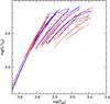 |
Fig. 1 HRD of the AGB phase of the Z=0.008, 1.6 M⊙ (solid line) and 1.8 M⊙ (dashed line) models, respectively. |
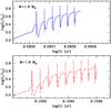 |
Fig. 2 Time evolution of the bolometric luminosity of the Z = 0.008, 1.6 M⊙ (solid line) and 1.8 M⊙ (dashed line) AGB tracks displayed in Fig. 1. |
The calculation of TP-AGB isochrones, however, are complicated by the following two issues:
-
The extremely short evolutionary timescales along the AGB (andin particular along the TP-AGB) phase, negligible compared tothe lifetime until the end of central He burning, and comparable tothe duration of the star formation episode. Any given isochroneage is therefore an idealization, and stars on the TP-AGB can be inany phase of pulse episodes.
-
The very irregular shape of the AGB tracks in the HRD, that can change substantially for small variations of the initial mass, as shown by the Hertzsprung-Russell diagram (HRD) of Fig. 1. We emphasize that the irregularity in the tracks shown arise mainly from that in the evolution of Teff, resulting from the complex interplay between a changing surface composition, opacities, mass loss, and induced structural changes. Luminosities, in contrast, behave much more regularly, as shown in Fig. 2. Notice how both models (1.6 and 1.8 M⊙, Z = 0.008) do reach similar minimum Teff along the AGB. The detailed Teff evolution is the result of the complicated interplay between opacities, surface C/O ratio, initial mass, and mass loss, but in general the two tracks attain similar Teff for similar actual mass and surface C/O ratio. When the C/O ratio reaches values around 2, the opacity becomes less sensitive to these abundances. At the end of the TP-AGB phase, both models having almost the same actual mass, in spite of different surface C/O ratios (~2.5 vs. ~2.0, the higher value for the model with initial mass equal to 1.6 M⊙) the final Teff is essentially the same.
To avoid potential spurious effects due to interpolations amongst the AGB phase of our adopted model grid, we proceeded as follows:
-
For a fixed initial chemical composition and age, we calculated isochrones from the MS to the end of the early-AGB (E-AGB) using the methods described in Prather (1976), Bergbusch & VandenBerg (1992), and Pietrinferni et al. (2004). Each isochrone is made of 1300 points. The E-AGB phase comprises 200 points. Isochrones were calculated for ages equal to the lifetime at the beginning of the AGB phase of the set of computed AGB tracks (τ in Table 1).
-
We took the evolutionary track of the mass whose lifetime at the beginning of the AGB phase corresponds to the age of the corresponding isochrone, as being representative of the isochrone AGB.
We call this composite sequence the evolutionary HRD of an SSP, and have therefore calculated evolutionary HRDs only for ages corresponding to the TP-AGB age of the masses in our grid. We did not consider intermediate values of the age because this requires an interpolation in mass amongst TP-AGB tracks. In principle, this interpolation should be avoided because of the extremely short timescales and the wide loops in the HRD during the TP-AGB phase, with no regular pattern at varying mass – especially for the lower masses – that would potentially cause a large uncertainty in the HRD evolution of the interpolated track. This becomes evident when considering the underlying idea of equivalent evolutionary points (Prather 1976; Pietrinferni et al. 2004) for the usual isochrone strategy.
Given the hybrid nature of our evolutionary HRDs, and the aim of determining the fluctuations of the integrated magnitudes sensitive to AGB stars, we had to resort to a non-standard way to determine the integrated flux of each SSP, which makes use of both MC simulations and analytical flux integrations:
-
At a given chemical composition, for each age we calculated synthetic HRDs of both E-AGB (the reason for including the E-AGB phase also is explained below) and TP-AGB phase. Given that these phases are represented by the evolutionary track of a single mass, the synthetic HRD has been calculated by randomly drawing age values within the range covered by the full AGB phase, with a uniform probability distribution. Interpolation in age along the track provided the HRD location of a representative synthetic AGB object. For each age and chemical composition we computed five sets of 100 realizations of the representative AGB, for numbers of stars equal to 10, 30, 100, 300, and 1000, respectively. Examples of MC HRDs of the AGB phase are shown in Fig. 3. For each realization and each number of TP-AGB objects, we calculated the integrated fluxes by simply adding up the spectra of each synthetic star.
-
We integrated the fluxes analytically along the corresponding isochrones from the MS to the end of central He-burning, using a Kroupa IMF (Kroupa 2001).
-
The choice of the IMF integration constant has been tied to the number of stars along the corresponding TP-AGB phase, as follows. There is a region of overlap between the MC simulations and the isochrones, that is the E-AGB phase. From each MC simulation of the AGB, we determined the number of E-AGB objects, to be compared with the number of E-AGB stars predicted by the analytical integration along the isochrone with the Kroupa IMF. The IMF integration constant was, therefore, obtained by imposing that the integration along the E-AGB part of the isochrone yields the same number of stars of the corresponding MC simulation. The integrated flux from the main sequence to the end of the TP-AGB phase was finally computed by summing up the integrated flux from the E-AGB + TP-AGB MC simulation, and the flux from the isochrone integration up to the end of central He-burning.
-
With the IMF integration constant fixed, we also determined the total evolving mass of the SSP (i.e. the stellar mass excluding remnants like white dwarfs, neutron stars and black holes) for each number of AGB stars in the MC simulations. Masses below 0.5 M⊙ and down to 0.1 M⊙, are assumed to contribute only to the total mass budget, but not to the fluxes. As a rough guideline, for our two selected metallicities and age ranges, 10, 100, and 1000 AGB objects correspond to ≈104 − 105M⊙, ≈ 105 − 106M⊙, and ≈ 106 − 107M⊙ of evolving stars, respectively (the exact values depend on age and initial chemical composition).
This whole procedure to calculate integrated fluxes was repeated again using the same AGB tracks, but with the evolution of L–Teff with time smoothed as discussed in Sect. 3.2 of Paper I, and shown in Fig. 4. These smooth versions of the tracks (that preserve the correct evolutionary timescales of the original calculations) are calculated using an analytical fit to the original track by employing second order polynomials. Notice how in the example displayed in Fig. 4, the smooth track differs from the original track during the E-AGB phase also. In other cases, the E-AGB evolution is almost unchanged. These smooth tracks will be employed in the next section to assess quantitatively the impact of this procedure on the resulting integrated magnitudes.
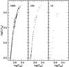 |
Fig. 3 Examples of Monte Carlo simulations of the AGB phase for Z = 0.008, t = 1.19 Gyr (log (t) = 9.08), and the labelled numbers of AGB stars. Each panel shows one out of 100 MC realization of the respective number of AGB stars. |
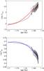 |
Fig. 4 Evolution with age of bolometric luminosity (top) and effective temperature (bottom) of the AGB track by WF09 with Z = 0.008 and M = 2 M⊙ (corresponding to the log (t) = 9.08 isochrone), and the corresponding smooth version (coloured lines) calculated as in Paper I. |
Mean values of the fractional AGB contribution to the total luminosity in the 2MASS Ks-band (Skrutskie et al. 1997) for our integrated stellar populations as a function of age (Cols. 2 and 6).
3. Theoretical predictions
We begin the presentation of our results by discussing the contribution of the AGB to the integrated K-band magnitude, denoted as  , of SSPs (we chose the 2MASS Ks-band, Skrutskie et al. 1997). This quantity is very sensitive to the AGB (see, for example, Marigo et al. 2011) and is frequently used as a standard diagnostics of AGB calculations (e.g., Mucciarelli et al. 2006; Ko et al. 2013). Table 2 summarizes the mean values obtained for our MC calculations at Z = 0.004 and Z = 0.008. We stress again that the population ages are determined by the underlying mass for which the AGB evolution was calculated (Sect. 2.3), and therefore are slightly different for the two representative mixtures. The spreads around the mean values were determined from the 1σ-ranges of the 100 MC simulations for each case.
The maximum contribution of AGB stars to the total K-band luminosity happens around an age t = 1.19 Gyr (log (t) ~ 9.08) for Z = 0.008, in agreement with, for example, the behaviour found by Marigo et al. (2010, Fig. 5). For the case Z = 0.004, the almost constant AGB fraction with age also agrees with results shown in Marigo et al. (2010), but smaller variations occuring on short timescales, as visible in that paper are no longer discernible because of our restricted number of isochrone ages. The maximum of the AGB contribution to the integrated Ks-band magnitude from the models is around 1.05 Gyr (log (t) ~ 9.04).
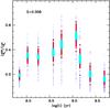 |
Fig. 5 Distribution of the |
The effect of statistical fluctuations for small numbers of AGB stars is very evident. The mean value of  at fixed age and Z is systematically lower for small samples because of the lack of brighter (and shorter lived) AGB objects, and converges to a stable value only when the number of AGB stars reaches ~100. The 1σ dispersion around the mean at fixed age and metallicity is obviously also a strong function of the number of AGB stars, decreasing with increasing number of AGB objects. The maximum of the AGB contribution is found at ages around log (t) = 9.0–9.1, with a slow rise at younger ages followed by a fast drop at older ages.
Figure 5 graphically displays the results for the Z = 0.008 case and the whole age range covered by our calculations. It is very evident, especially in the simulations for 10 and 100 AGB stars –as also demonstrated by the data in Table 2– how the full range of values spanned by the MC realizations at fixed number of AGB objects is a function of age. The total spread at fixed age is higher at those ages where the mean value of is higher, that is, when the AGB contribution to the integrated luminosity in the K-band is maximized. The case with ten AGB stars is particularly interesting because ten (or fewer) is the typical number of objects populating the AGB of LMC and SMC clusters employed to test the integrated near-IR SSP colours (see, e.g., Mucciarelli et al. 2006; Noël et al. 2013).
To delve further into this issue, we show as an example in Fig. 6 the distribution of values for Z = 0.008, an age of 1.19 Gyr (log (t) = 9.08, when the AGB contribution attains its maximum), and the same three values of the total number of AGB stars as in Fig. 5. It is important to notice that for small numbers of stars, the mean value, which is lower thanin the case of more populated AGBs, does not coincide with a pronounced maximum in the number distribution. The probability of encountering a cluster with only ten AGB stars at any value within a range between ~0.1 and and ~0.7, has an almost flat distribution. This means that one expects a broad, almost uniform distribution of observed ratios, when comparing models with individual Magellanic Cloud clusters. This will be discussed in the next section.
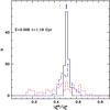 |
Fig. 6 Number distribution of |
The spread in causes a spread of the predicted IR colours (see, e.g., Santos & Frogel 1997; Lançon & Mouhcine 2000; Bruzual 2002; Raimondo 2009, for past analyses of statistical fluctuations on IR colours due to the AGB population), as demonstrated by the data in Table 3, which shows (V − Ks) colours corresponding to the same values of Table 2. Figure 7 graphically displays the distribution of (V − Ks) colours from the MC simulations for Z = 0.008 reported in Table 3. Notice how this colour displays a steady increase with age, for ages above log (t) ~ 9.1, after the AGB contribution to the K-band has dropped significantly due to the increasing contribution of RGB stars.
The general behaviour of the statistical fluctuations is similar to the case of the ratio. For the relevant case of ten AGB objects discussed before, the full colour range at the age when the AGB contribution is the largest (log (t) = 9.08) spans ≈1 mag. Figure 8 displays the distribution of (V − Ks) colours for the same parameters as in Fig. 6. The probability of encountering a cluster with only ten AGB stars at any colour between 2.8–3.0 and ~1.9 mag has again an almost flat distribution, and there is a blueward bias of ~0.1 mag for the corresponding mean value, compared to the case of more populated AGBs.
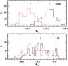 |
Fig. 9 Number distribution of integrated Ks magnitudes obtained from the original (solid line) and smooth (dash-dotted line) AGB tracks, for the case with age t = 1.19 Gyr (log (t) = 9.08) and Z = 0.008, with 10 (lower panel) and 1000 (upper panel) AGB stars. Average values are marked at the top of the diagrams. |
We now compare the results obtained from the full AGB calculations with the case of employing the smooth AGB tracks of Paper I (see Fig. 4) to assess the presence of systematic effects for the contribution of the AGB to the integrated light, due to the smoothing process. To this purpose, we calculated sets of integrated magnitudes for Z = 0.004 and Z = 0.008 as described in the previous section, but employing the smooth version of WF09 AGB tracks. As expected, blue-optical filters are unaffected by the smoothing of the AGB, whereas integrated magnitudes in filters like JHK display some differences, although these are generally minor. Obviously, the larger discrepancies are found at ages where the AGB contribution to the integrated light is larger, e.g., around log (t) = 9.0. If we focus on the integrated magnitude in the Ks-band, the mean values differ by at most ~0.10 mag for the cases with log (t) = 9.02, Z = 0.004, and log (t) = 9.08, Z = 0.008, almost independent of the number of AGB stars in the MC simulations. In most cases, however, these differences are within a few 0.01 mag. Figure 9 displays, as an example, the number distribution of integrated Ks magnitudes obtained from the original and smooth AGB tracks, for the case with log (t) = 9.08 and Z = 0.008 (for both 10 and 1000 AGB stars). The difference of the mean values is 0.10 mag, with smooth tracks providing brighter integrated magnitudes. In the case of 1000 stars the differences of the overall Ks-band magnitude distributions are obvious; as for the samples with ten stars, although the overall distributions seem similar (almost flat over a large magnitude range), in addition to the differences of the mean values, a KS-test returns a 99% probability that the two distributions are not the same.
The origin of these differences in the mean values of the integrated magnitudes can be traced back not to the TP-AGB phase, but to the differences along the E-AGB between the smooth analytic approximations of Paper I and the complete calculations. As shown by Fig. 4, the smooth AGB track corresponding to log (t) = 9.08 and Z = 0.008 is on average overluminous during the E-AGB phase, and this produces the different mean integrated Ks magnitude. Smoothing the TP-AGB part of the evolution does not affect appreciably the final integrated magnitudes.
As for the 1σ dispersion around the mean magnitudes, it is generally only slightly reduced in the case of the smoothed tracks, for simulations up to 100 AGB stars. The reduction of the dispersion is enhanced when the AGB contribution peaks. To give more quantitative estimates of the maximum expected reduction, populations of 1000, 100, and 10 objects display 1σ dispersions equal to ~0.03, 0.10, and 0.30 mag for log (t) ~ 9.0, respectively, but they are almost independent of age and Z. These are reduced by ~0.02 and ~0.05–0.10 mag for the case of 100 and 10 AGB stars, respectively, when smooth models are employed.
We conclude this section by comparing selected integrated optical and IR colours we obtained with WF09 calculations for both AGB and pre-AGB phases (we display the full set of MC simulations with 1000 stars for each age), with the results of Paper I. We also compare our findings with the predictions by Maraston (2005) based on the fuel consumption theorem formalism, Marigo et al. (2008), who made use of sophisticated synthetic AGB calculations, and finally “BaSTI TP-AGB extended” (Percival et al. 2009, the set that includes MS convective core overshooting), which employs the synthetic AGB treatment described by Cordier et al. (2007). Figure 10 displays the various predictions as a function of age for Z = 0.008 in the Bessel-Brett system. Our colours and Paper I results in this case do not include the effect of circumstellar dust, to be consistent with the other models displayed. The effect of dust is however completely negligible for the (B − V) colour, and amounts to just a few hundredths of a magnitude for (J − K) and (V − K).
We start by considering Paper I models. We recall that the differences to our results involve the pre-AGB evolution, taken from independent models, the smoothing of the AGB tracks, and their shift, in both Teff and luminosity, to match the beginning of the AGB phase to the pre-AGB isochrones. The size of these shifts displayed a strong dependence on mass and metallicity of the models (see Fig. 2 in Paper I). At this metallicity, the maximum shift in Teff is of about ~700 K at M = 1 M⊙. More typical values for the other masses are of the order of 250 K. As for the luminosity, the shifts are at most Δ(L/L⊙) ~ 0.1.
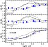 |
Fig. 10 Integrated optical and near-IR colours as a function of age for Z = 0.008, as obtained in this paper (open squares – results for MC simulations with 1000 AGB stars; notice the overlap of the symbols in the upper two panels, due to low magnitude fluctuations that mimic solid squares), Paper I (dotted line), BaSTI (dashed line), Marigo et al. (2008) and Maraston (2005) (solid and dot-dashed, respectively) population synthesis models (see text for details). |
In spite of these differences, both optical (unaffected by the AGB) and near-IR colours show a very good agreement with our results. Clearly, the various effects cancel out to provide such a good agreement with fully consistent colours calculated here. The only major differences appear for ages below 100 Myr, before the onset of the AGB phase, with our colours being systematically redder. As for the comparison with BaSTI, the agreement with our results is surprisingly good also in this case, even below 100 Myr. There is just a small systematic offset in (J − K), for the age range dominated by the AGB, with BaSTI colours being redder by about 0.05–0.10 mag. Notice the moderate red spike of the Marigo et al. (2008) and BaSTI results at log (t) ~ 9.1–9.2 for the reasons discussed in the previous section. The spike is more evident in (J − K) and (V − K) for BaSTI models, whereas it does not appear in the (J − K) colours from Marigo et al. (2008).
In the case of Maraston (2005) and Marigo et al. (2008) models, Fig. 10 shows a much larger disagreement with our results. Our near-IR colours are systematically bluer between log (t) ~ 8.3 and log (t) ~ 9.3, where the AGB controls the IR luminosity, by up to ~0.4–0.5 mag in (J − K), and ~1 mag in (V − K). In the same age range, optical colours display a negligible difference with Marigo et al. (2008) results, whereas Maraston (2005) are still systematically redder, albeit by a smaller amount.
3.1. Fluctuations of the RGB integrated luminosity
So far we have focussed on the statistical fluctuations of the AGB contribution to integrated magnitudes and colours. We will continue to focus to on these statistical fluctuations in the rest of the paper. However, also the contribution of RGB stars can fluctuate statistically, when the number of objects is small. This is due to the relatively short evolutionary timescales along the bright part of the RGB, especially close to the tip. To this purpose, we have performed some numerical tests by calculating integrated magnitudes with synthetic HRDs for the RGB part of our isochrones as well, with the total number of RGB objects predicted by the analytical integration for a fixed age, chemical composition, and number of AGB stars. We performed multiple MC realizations of both RGB and AGB phases to study how the fluctuations of the IR integrated magnitudes and colours discussed before are modified by the inclusion of statistical effects along the RGB.
We found that for ages up to log (t) ~ 9.1 (about 1.2 Gyr) the additional fluctuations are negligible compared to those induced by the AGB, for every cluster mass explored. This is not surprising, given that the contribution of the RGB phase to the integrated magnitudes is negligible in this age range. For ages above this threshold, after the RGB transition, the fluctuations due to RGB and AGB become comparable in size, and therefore the total 1σ fluctuation of the flux will be ~1.4 times the value due only to the AGB. This corresponds roughly to the case, when only statistical fluctuations due to AGB stars are considered, of decreasing the number of AGB stars by a factor about 3 compared to the actual value. In the next section, with comparisons between theoretical predictions and observations, we neglect to account for this additional spread coming from RGB stars when considering ages above log (t) ~ 9.1 because its inclusion does not affect the overall agreement – or lack of agreement – between theory and observations.
4. Observational tests
The comparison of Fig. 10 displays appreciable differences of AGB-dominated colours between our calculations and some of the independent results displayed there. These differences result from the underlying models, and not from our new isochrone approach, as was just shown. This provides an additional motivation to address the issue of the consistency of our present calculations with empirical constraints.
We start by comparing the predicted ratios with the data by Ko et al. (2013). These authors provided data for about 100 LMC clusters in the age range spanned by our models, and assigned an age to each cluster primarily by means of isochrone fitting. For about 20 clusters they resorted to literature estimates, mainly obtained from integrated colour analysis, and assumed Z = 0.008 for the whole sample. Here we will compare the data with theoretical predictions for Z = 0.008 at ages below log (t) = 9.3, Z = 0.004 above log (t) = 9.5, and both metallicities for log(t) around 9.3, as discussed in the following comparisons with integrated colours.
Figure 11 displays the results for the whole sample divided into three  ranges. Error bars for individual clusters are also displayed, taken from Ko et al. (2013). We compared these data with the theoretical predictions from our suite of MC simulations. The K-band integrated luminosity with fixed number of AGB stars has a strong dependence on the age (at fixed metallicity). In the intermediate luminosity range, we selected simulations with typically ten AGB stars that produce integrated K-band luminosities within the selected range (in the theoretical calculations we employed
  , as in Ko et al. 2013). For the fainter range, we also employed the simulations with ten AGB objects. This is the lowest number chosen for our simulations, but they still provide integrated total luminosities brighter than the observed luminosity, whilst the two brightest clusters have been compared with the appropriate simulations for 30 AGB stars.
It is very important to notice how the values for the faintest sample are scattered almost uniformly over extremely large ranges, essentially as predicted for SSPs with a small number of AGB stars (see previous section). The intermediate luminosity sample, although of a smaller size, starts to display a structure in the -age plane that matches the theoretical predictions. The two most luminous clusters displayed in the top panel, also match the theoretical predictions very well.
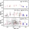 |
Fig. 11
|
To minimize the uncertainties of low-number statistics, we followed the approach by González et al. (2004), Pessev et al. (2008), Noël et al. (2013), and Ko et al. (2013), and constructed artificial superclusters by adding the fluxes of individual, resolved clusters that lie in a sufficiently narrow range of metallicity and age. In general terms, the requirements of this method are obvious: observations and metallicity determinations should best be from a homogeneous set of data, and be analysed consistently, and cluster ages should be reliable. Second, to create a realistic supercluster this way, both metallicity and age range should ideally be very narrow, which tends to clash with the requirement of large AGB star numbers (e.g., several clusters).
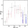 |
Fig. 12 As Fig. 11, except for superclusters obtained from the clusters sample by Ko et al. (2013). |
We grouped the clusters from the sample by Ko et al. (2013) in 0.3 dex wide age bins (the youngest bin centred at log (t) = 7.7), and added up both integrated total flux, and the AGB-only flux of each cluster in a given group, to produce ratios for seven superclusters. Ko et al. (2013) also calculated luminosity ratios for superclusters, but defined in slightly different age ranges compared to our choice. Error bars on the resulting values have been obtained by a simple error propagation of the errors for the individual clusters in each supercluster. Figure 12 compares these ratios with theoretical predictions for the number of AGB stars that best matches the K-band integrated luminosity of the closest supercluster, typically equal to 30 objects (still a reasonably low number). The assumption behind the comparison with theory is the following: if the theory is in agreement with observations and each supercluster is the equivalent of one theoretical MC realization with the appropriate number of AGB stars, the observational points (within their horizontal error bars) should overlap with the distribution of theoretical MC simulations at the appropriate age.
It is clear that the data follow our predictions very nicely and overlap (within the individual error bars) with the distribution of MC results. Even if the data formally display a maximum at log (t) = 8.6, while the models predict that the mean value of has a maximum at log (t) = 9.08, there is no real contradiction, given that at log (t) ~ 8.5 the MC simulations predict a range of values that nicely overlap with the observed value.
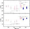 |
Fig. 13 Colours of the superclusters (see text for details) by Pessev et al. (2008), indicated by circles with error bars, and Noël et al. (2013), indicated by squares with error bars. The horizontal error bars denote the age bins covered by each supercluster. Predictions from models for Z = 0.008 (red dots) and Z = 0.004 (blue three-pointed stars) with a number of AGB stars corresponding to total masses a few times 105M⊙ are shown for comparison. |
As a next step we considered comparisons of selected integrated colours with empirical determinations from different sources. We start the comparison with superclusters from Pessev et al. (2008). The data were from Pessev et al. (2006) for 45 Magellanic Cloud clusters, with an additional 9 clusters taken from the literature; age estimates come from a variety of sources, mainly based (in the age range of our comparisons) on cluster colour–magnitude–diagrams rather than age-sensitive integrated colours. Their own 2MASS IR photometry was matched to optical photometry from other sources. Integrated fluxes were co-added to build several superclusters covering age ranges between log (t) = 8.3 and the age of the universe (see Table 5 of that paper), and the weighted mean colours with the corresponding errors are provided. Three of these superclusters lie in the age range spanned by our models. The number of combined clusters (of the order of ~10 per supercluster) gives typical masses of the order of a few times 105M⊙ for each supercluster. The mean metallicity of each supercluster equals [ Fe/H ] = −0.34 for log(t) between 8.3 and 9.0, [ Fe/H ] = −0.45 for log(t) between 9.0 and 9.3, and [ Fe/H ] = −0.52 for log(t) between 9.3 and 9.66. Integrated colours vs. age of these superclusters and our corresponding theoretical predictions are displayed in Fig. 13 as open circles. The horizontal error bar corresponds to the width of the age bin spanned by each supercluster. The error bar on the mean colours has the same size of the symbols.
A similar cluster sample was also investigated recently by Noël et al. (2013). They adopted age estimates for the individual clusters often (but not always) different from Pessev et al. (2008), also taken from a variety of literature sources, mainly from isochrone fitting. These authors also merge clusters into superclusters, spanning somewhat narrower age ranges. The typical masses estimated by the authors are again of order 105M⊙ for each supercluster, and we plot their data in Fig. 13 with open squares. The horizontal error bars correspond again to the width of the age bin spanned by each supercluster. As for the error in the colours, the authors provided the V-band luminosity-weighted standard deviation of the colours in each bin. This is different (much larger) from the error just due to the photometric uncertainties for individual clusters, and we did not display these colour error bars for the reasons we discuss below.
The same Fig. 13 shows also the predictions from our suite of MC calculations for the number of stars that more closely match the mass of the closest supercluster (typically, we need the results with 100 AGB stars). To follow the trend of mean supercluster [Fe/H] with age of Pessev et al. (2008) data, we employ the results for Z = 0.008, except for the two oldest ages. At ages of around log (t) = 9.3, we display results for both Z = 0.008 and Z = 0.004, whereas at the oldest age we show only the Z = 0.004 results. We assume that the trend [Fe/H] vs age for Noël et al. (2013) superclusters is consistent with Pessev et al. (2008), given that they employ a very similar cluster sample. Using colours in common to two different sets of superclusters from essentially the same cluster sample, which made use of different groupings and age estimates, should give us an idea of the uncertainties involved in the empirical determination of the supercluster colours.
The agreement with theory appears satisfactory in the (J − Ks) colour, for the age range between log (t) ~ 8.3 and log (t) ~ 9.0. At younger ages, theoretical colours seem too red, while they are too blue at older ages compared to Pessev et al. (2008) data. However, the oldest supercluster from Noël et al. (2013) does not show a substantial discrepancy with the models for Z = 0.008. In the case of (V − Ks) colour, only the ages above log (t) ~ 9.0 are satisfactorily matched with the models; at younger ages the models systematically appear too red.
Figure 14 displays a comparison of theoretical integrated colours with González et al. (2004) superclusters, in the age range spanned by our calculations. These authors have constructed superclusters from observed 2MASS integrated magnitudes of about 200 Magellanic Cloud clusters for which an s-parameter (Elson & Fall 1985, 1988) had been determined. The SWB-class of each supercluster was defined by the value of s, co-adding the individual clusters of each SWB class (Searle et al. 1980). Finally, ages of the various SWB classes were taken from Cohen (1982). No age estimates of the individual clusters are provided, and the mass of the superclusters is usually a factor of about ten higher than the superclusters by Noël et al. (2013) and Pessev et al. (2008).
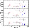 |
Fig. 14 As Fig. 13, except for the superclusters by González et al. (2004). The meaning of symbols is the same as in Fig. 13. |
Also in this case the horizontal error bars shown in the figure correspond to the width of the age bin spanned by each supercluster. As for the colours, we considered the authors’ estimate of the photometric errors (0.03 mag). The theoretical results displayed are from MC calculations with typically 1000 AGB stars (except for the two youngest ages), which approximately match the superclusters’ masses quoted by González et al. (2004). The metallicities of the theoretical results follow the same trend with age of the previous comparisons (from Pessev et al. 2008, superclusters), which is consistent with the metallicity ranges assigned by González et al. (2004) to each of their superclusters (following Cohen 1982).
For these data, the agreement with theory is good over the whole age range and the three colour combinations, apart from the supercluster centred around log (t) ~ 9.3. Notice that at the youngest ages there is no clear discrepancy between models and observations, contrary to what was found for Noël et al. (2013) and Pessev et al. (2008) superclusters. On the other hand, for the supercluster at log (t) ~ 9.3, the observed colours appear redder than theory, especially in the (J − Ks) and (H − Ks) colours. The same discrepancy in (J − Ks) is found in the comparison with Pessev et al. (2008) superclusters, but not with Noël et al. (2013) superclusters.
It may well be that this situation stems from the effect recently analysed in detail by Girardi et al. (2013). The basic idea is that for ages at which the RGB starts to develop (transition to electron degenerate He-cores), the approximation of constant initial mass for the AGB breaks down (see Girardi et al. 2013, for a thorough discussion), and the use of our approximation to calculate the AGB evolution underestimates the contribution of these stars to the integrated luminosity by up to a factor ~2. The narrow age range where this happens is at log (t) ~ 9.2 in our models, which is within the age interval covered by the discrepant superclusters.
To further investigate this issue, we have considered all objects in the González et al. (2004) supercluster spanning the range log (t) = 9.0–9.7. Most of the clusters are in common with Pessev et al. (2008) and Noël et al. (2013) studies, although in these latter works they are grouped into two superclusters rather than one. According to the individual age estimates from these two studies, the majority of the objects have an age log (t) ~ 9.15–9.3, e.g. around the critical narrow age range where our approximation to calculate integrated colours breaks down. There is, therefore, a possibility that the discrepancies seen around log (t) ~ 9.2–9.3 in Figs. 14 and 13, but that do not show up in Fig. 12, might be due to the effect discussed by Girardi et al. (2013). This depends on the exact value of the cluster ages assigned by the authors, whether clusters around the critical age are grouped into just one superclusters, and the extent of the dilution effect due to objects away from the transition to electron degenerate He-cores, which are, however, included in the same supercluster.
5. Conclusions
Star clusters in the Magellanic Clouds are of special interest as they cover an age range in which stars of low- and intermediate mass develop into double-shell burning objects populating the AGB, and are massive enough to host at least a few AGB stars. Such clusters, therefore, serve as template and calibration objects for population synthesis aimed at understanding the star formation history of distant galaxies during the last few hundred million to a few billion years. Observations, such as those shown in Fig. 11, however, display a large variation of integrated IR colours for clusters of presumably very similar age and composition. Thus it is unclear to what accuracy theoretical population synthesis models could be calibrated or verified against such variations.
It was recognized early on (Chiosi et al. 1988; Frogel et al. 1990) that the low number of AGB stars in individual clusters results in statistical fluctuations of the AGB integrated luminosity that, given the important contribution of late-type luminous stars to the integrated IR-light, explains the variation of IR integrated colours. In this paper, we presented new theoretical predictions of near-IR colours of intermediate-age populations, and tested them against data about clusters in the LMC and SMC, taking their low number of AGB-stars into account.
Our predictions rest on the new WF09 fully evolutionary AGB stellar models for stars of low and intermediate mass, and a detailed treatment of the effect of their surrounding dust shells, to achieve the most realistic description of their stellar energy distribution. In Paper I, we already introduced the new AGB models and the treatment of the dusty envelope, and applied it to observations of galaxies. In that paper, however, WF09 AGB tracks were smoothed out (to calculate AGB isochrones) and shifted in both luminosity and Teff to match an independent set of isochrones that model the pre-AGB evolution. Here we employ the full evolution until the end of the TP-AGB phase from WF09 calculations.
One new aspect of our predictions is the treatment of the TP-AGB phase in the construction of isochrones (Sect. 2.3). We use an MC scheme to populate what we call an evolutionary HRD with a given number of AGB stars, comparable to that of observed clusters, and combine it with a standard isochrone for earlier evolutionary phases. This way we are able to take into account all temperature and luminosity variations that occur during the TP-AGB cycles as well as the statistical fluctuations due to finite star numbers. Our results, presented in Sect. 3, quantitatively demonstrate the possible range of both IR colours (we consider (V − Ks) in Fig. 7) and the contribution of AGB stars to the integrated Ks-luminosity (Fig. 5), how they approach a mean value for large (~1000) numbers of AGB stars, and how they distribute almost uniformly over a wide range for low numbers (the case of 10 AGB stars). In (V − Ks) the colour of any cluster can vary by as much as ±0.37 mag (1σ; Table 3). In fact, our models cover a range up to ~1.2 mag for ages close to 1 Gyr, when AGB stars are most dominant. We have also shown that the luminosity and Teff variations during the TP-AGB cycles do not significantly contribute to the total statistical fluctuations of the AGB integrated light. Hence, interpolations amongst smoothed AGB-tracks as in Paper I, when carefully constructed, can also be used. They allow construction of conventional isochrones for any desired age, while our, in principle, more accurate method is restricted by default to the ages of the available stellar model tracks. We have then extended our analysis to investigate the additional contribution of the fluctuations of the RGB integrated luminosity for poorly populated clusters. We found that, as expected, the RGB contribution is negligible for ages below log (t) ~ = 9.1 (ages younger than the transition to electron degenerate He-cores), while it becomes comparable to the AGB fluctuations at older ages.
In terms of consequences for population synthesis of younger stellar clusters, e.g., in star forming regions of distant galaxies, our results imply that for any given age in the range between ~0.1 and ~1 Gyr, infrared colours may vary because to statistical fluctuations in the number of AGB stars, to an extent that the cluster age cannot be determined more accurately than a factor ~10. This is already implied by the observational data used in this paper, but substantiated now by our theoretical models.
We have taken these AGB statistical fluctuations into account to compare our predictions with empirical data on Magellanic Cloud clusters, which are the standard bench tests of near-IR population synthesis models. The comparison with empirical estimates of the ratio by Ko et al. (2013) shows very good agreement in general: when considering the appropriate number of AGB stars, the statistical scatter of our predictions covers the observed distribution, and the variation of Ks-band luminosity with age for stacked clusters (or supercluster) also agrees very well with their data (Figs. 11 and 12).
When considering integrated near-IR colours, the level of agreement with empirical data for several samples of superclusters (Noël et al. 2013; Pessev et al. 2008; González et al. 2004) depends somewhat on the selected colour, but also on the sample. Clearly, the construction of superclusters as well as the individual observations themselves, are sometimes not consistent. These discrepancies need clarification, and should be a warning to population synthesis models that require calibration with such observed superclusters. In general, our predictions pass the observational tests well, and can also be properly applied to study individual clusters hosting a low number of AGB stars.
A comparison with integrated colours from other population synthesis models, including the results of Paper I, reveals significant discrepancies with results from Marigo et al. (2008) and Maraston (2005). Noël et al. (2013) have already discussed how these models disagree (they are generally too red) with the integrated colours of their superclusters for ages between ~108 and ~109 years. The agreement with the model of Paper I and with the BaSTI-model by Cordier et al. (2007), in contrast, is excellent.
In summary, we have presented a statistical approach to model integrated colours of intermediate-age populations with a small number of stars that makes use of new state-of-the-art stellar evolution models, accounts for the effect of dusty envelopes, quantifies statistical fluctuations and matches observations of individual Magellanic Cloud clusters as well as artificial superclusters well. The predictive power of these theoretical models, which are not calibrated beforehand on a specific set of observations, should be sufficient for wider applications to other stellar populations spanning a larger range of metallicities and/or more complex star formation histories.
Acknowledgments
We thank N. E. Noël for discussion about her results, and S. Cassisi for comments on an earlier draft of the paper. M.S. is grateful to the Max Planck Institut für Astrophysik for hospitality and support for several visits, during which most of this work was carried out.
References
- Allard, F., & Hauschildt, P. H. 1995, ApJ, 445, 433 [NASA ADS] [CrossRef] [Google Scholar]
- Anders, P., Bissantz, N., Fritze-v. Alvensleben, U., & de Grijs, R. 2004, MNRAS, 347, 196 [NASA ADS] [CrossRef] [Google Scholar]
- Bergbusch, P. A., & VandenBerg, D. A. 1992, ApJS, 81, 163 [NASA ADS] [CrossRef] [Google Scholar]
- Bertelli, G., Bressan, A., Chiosi, C., Fagotto, F., & Nasi, E. 1994, A&AS, 106, 275 [NASA ADS] [Google Scholar]
- Bessell, M. S., Brett, J. M., Wood, P. R., & Scholz, M. 1989, A&AS, 77, 1 [NASA ADS] [Google Scholar]
- Bessell, M. S., Brett, J. M., & Scholz, M. W. P. R. 1991, A&A, 89, 335 [Google Scholar]
- Bruzual, G. 2002, in Extragalactic Star Clusters, eds. D. P. Geisler, E. K. Grebel, & D. Minniti, IAU Symp., 207, 616 [Google Scholar]
- Bruzual, G., & Charlot, S. 2003, MNRAS, 344, 1000 [NASA ADS] [CrossRef] [Google Scholar]
- Cassarà, L. P., Piovan, L., Weiss, A., Salaris, M., & Chiosi, C. 2013, MNRAS, 436, 2824 [NASA ADS] [CrossRef] [Google Scholar]
- Chiosi, C., Bertelli, G., & Bressan, A. 1988, A&A, 196, 84 [Google Scholar]
- Cohen, J. G. 1982, ApJ, 258, 143 [NASA ADS] [CrossRef] [Google Scholar]
- Conroy, C., & Gunn, J. E. 2010, ApJ, 712, 833 [NASA ADS] [CrossRef] [Google Scholar]
- Cordier, D., Pietrinferni, A., Cassisi, S., & Salaris, M. 2007, AJ, 133, 468 [NASA ADS] [CrossRef] [Google Scholar]
- Elitzur, M., & Ivezić, Ž. 2001, MNRAS, 327, 403 [NASA ADS] [CrossRef] [Google Scholar]
- Elson, R. A. W., & Fall, S. M. 1985, ApJ, 299, 211 [NASA ADS] [CrossRef] [Google Scholar]
- Elson, R. A., & Fall, S. M. 1988, AJ, 96, 1383 [NASA ADS] [CrossRef] [Google Scholar]
- Ferguson, J. W., Alexander, D. R., Allard, F., et al. 2005, ApJ, 623, 585 [NASA ADS] [CrossRef] [Google Scholar]
- Fluks, M. A., Plez, B., The, P. S., et al. 1994, A&AS, 105, 311 [NASA ADS] [Google Scholar]
- Frogel, J. A., Mould, J., & Blanco, V. M. 1990, ApJ, 352, 96 [NASA ADS] [CrossRef] [Google Scholar]
- Girardi, L., Marigo, P., Bressan, A., & Rosenfield, P. 2013, ApJ, 777, 142 [NASA ADS] [CrossRef] [Google Scholar]
- González, R. A., Liu, M. C., & Bruzual, G. 2004, ApJ, 611, 270 [NASA ADS] [CrossRef] [Google Scholar]
- Grevesse, N., & Noels, A. 1993, Phys. Scripta, T47, 133 [Google Scholar]
- Iglesias, C. A., & Rogers, F. J. 1996, ApJ, 464, 943 [NASA ADS] [CrossRef] [Google Scholar]
- Into, T., & Portinari, L. 2013, MNRAS, 430, 2715 [NASA ADS] [CrossRef] [Google Scholar]
- Ivezic, Z., & Elitzur, M. 1997, MNRAS, 287, 799 [NASA ADS] [CrossRef] [Google Scholar]
- Izzard, R. G., Tout, C. A., Karakas, A. I., & Pols, O. R. 2004, MNRAS, 350, 407 [NASA ADS] [CrossRef] [Google Scholar]
- James, P. A., Salaris, M., Davies, J. I., Phillipps, S., & Cassisi, S. 2006, MNRAS, 367, 339 [NASA ADS] [CrossRef] [Google Scholar]
- Karakas, A. I., Campbell, S. W., & Stancliffe, R. J. 2010, ApJ, 713, 374 [NASA ADS] [CrossRef] [Google Scholar]
- Kitsikis, A. 2008, Ph.D. Thesis, Ludwig-Maximilians-Universität München, Germany [Google Scholar]
- Ko, Y., Lee, M. G., & Lim, S. 2013, ApJ, 777, 82 [NASA ADS] [CrossRef] [Google Scholar]
- Kroupa, P. 2001, MNRAS, 322, 231 [NASA ADS] [CrossRef] [Google Scholar]
- Lançon, A. & Mouhcine, M. 2000, in Massive Stellar Clusters, eds. A. Lançon, & C. M. Boily, ASP Conf. Ser., 211, 34 [Google Scholar]
- Lejeune, T., Cuisinier, F., & Buser, R. 1998, A&AS, 130, 65 [NASA ADS] [CrossRef] [EDP Sciences] [Google Scholar]
- Maraston, C. 2005, MNRAS, 362, 799 [NASA ADS] [CrossRef] [Google Scholar]
- Marigo, P., & Girardi, L. 2007, A&A, 469, 239 [NASA ADS] [CrossRef] [EDP Sciences] [Google Scholar]
- Marigo, P., Girardi, L., Bressan, A., et al. 2008, A&A, 482, 883 [NASA ADS] [CrossRef] [EDP Sciences] [Google Scholar]
- Marigo, P., Girardi, L., Bressan, A., et al. 2010, in IAU Symp. 262, eds. G. R. Bruzual, & S. Charlot, 36 [Google Scholar]
- Marigo, P., Bressan, A., Girardi, L., et al. 2011, in Why Galaxies Care about AGB Stars II: Shining Examples and Common Inhabitants, eds. F. Kerschbaum, T. Lebzelter, & R. F. Wing, ASP Conf. Ser., 445, 431 [Google Scholar]
- Mucciarelli, A., Origlia, L., Ferraro, F. R., Maraston, C., & Testa, V. 2006, ApJ, 646, 939 [NASA ADS] [CrossRef] [Google Scholar]
- Noël, N. E. D., Greggio, L., Renzini, A., Carollo, C. M., & Maraston, C. 2013, ApJ, 772, 58 [Google Scholar]
- Percival, S. M., Salaris, M., Cassisi, S., & Pietrinferni, A. 2009, ApJ, 690, 427 [NASA ADS] [CrossRef] [Google Scholar]
- Pessev, P. M., Goudfrooij, P., Puzia, T. H., & Chandar, R. 2006, AJ, 132, 781 [NASA ADS] [CrossRef] [Google Scholar]
- Pessev, P. M., Goudfrooij, P., Puzia, T. H., & Chandar, R. 2008, MNRAS, 385, 1535 [NASA ADS] [CrossRef] [Google Scholar]
- Pietrinferni, A., Cassisi, S., Salaris, M., & Castelli, F. 2004, ApJ, 612, 168 [NASA ADS] [CrossRef] [Google Scholar]
- Piovan, L., Tantalo, R., & Chiosi, C. 2003, A&A, 408, 559 [NASA ADS] [CrossRef] [EDP Sciences] [Google Scholar]
- Prather, M. 1976, Ph.D. Thesis, Yale University, USA [Google Scholar]
- Raimondo, G. 2009, ApJ, 700, 1247 [NASA ADS] [CrossRef] [Google Scholar]
- Santos, Jr., J. F. C., & Frogel, J. A. 1997, ApJ, 479, 764 [NASA ADS] [CrossRef] [Google Scholar]
- Searle, L., Wilkinson, A., & Bagnuolo, W. G. 1980, ApJ, 239, 803 [NASA ADS] [CrossRef] [Google Scholar]
- Skrutskie, M. F., Schneider, S. E., Stiening, R., et al. 1997, in The Impact of Large Scale Near-IR Sky Surveys, eds. F. Garzon, N. Epchtein, A. Omont, B. Burton, & P. Persi, Astrophys. Space Sci. Lib., 210, 25 [Google Scholar]
- van Loon, J. T., Cioni, M., Zijlstra, A. A., & Loup, C. 2005, A&A, 438, 273 [NASA ADS] [CrossRef] [EDP Sciences] [Google Scholar]
- Ventura, P., & Marigo, P. 2010, MNRAS, 408, 2476 [NASA ADS] [CrossRef] [Google Scholar]
- Wachter, A., Schröder, K.-P., Winters, J. M., Arndt, T. U., & Sedlmayr, E. 2002, A&A, 384, 452 [NASA ADS] [CrossRef] [EDP Sciences] [Google Scholar]
- Weiss, A., & Ferguson, J. W. 2009, A&A, 508, 1343 [NASA ADS] [CrossRef] [EDP Sciences] [Google Scholar]
- Weiss, A., & Schlattl, H. 2008, Ap&SS, 316, 99 [NASA ADS] [CrossRef] [Google Scholar]
- Zhang, F., Li, L., Han, Z., Zhuang, Y., & Kang, X. 2013, MNRAS, 428, 3390 [NASA ADS] [CrossRef] [Google Scholar]
All Tables
Mean values of the fractional AGB contribution to the total luminosity in the 2MASS Ks-band (Skrutskie et al. 1997) for our integrated stellar populations as a function of age (Cols. 2 and 6).
All Figures
|
Fig. 1 HRD of the AGB phase of the Z=0.008, 1.6 M⊙ (solid line) and 1.8 M⊙ (dashed line) models, respectively. |
| In the text | |
|
Fig. 2 Time evolution of the bolometric luminosity of the Z = 0.008, 1.6 M⊙ (solid line) and 1.8 M⊙ (dashed line) AGB tracks displayed in Fig. 1. |
| In the text | |
|
Fig. 3 Examples of Monte Carlo simulations of the AGB phase for Z = 0.008, t = 1.19 Gyr (log (t) = 9.08), and the labelled numbers of AGB stars. Each panel shows one out of 100 MC realization of the respective number of AGB stars. |
| In the text | |
|
Fig. 4 Evolution with age of bolometric luminosity (top) and effective temperature (bottom) of the AGB track by WF09 with Z = 0.008 and M = 2 M⊙ (corresponding to the log (t) = 9.08 isochrone), and the corresponding smooth version (coloured lines) calculated as in Paper I. |
| In the text | |
|
Fig. 5 Distribution of the |
| In the text | |
|
Fig. 6 Number distribution of |
| In the text | |
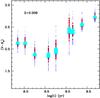 |
Fig. 7 Same as Fig. 5, but for the (V − Ks) colour. |
| In the text | |
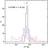 |
Fig. 8 As Fig. 6, but for the (V − Ks) integrated colour. |
| In the text | |
|
Fig. 9 Number distribution of integrated Ks magnitudes obtained from the original (solid line) and smooth (dash-dotted line) AGB tracks, for the case with age t = 1.19 Gyr (log (t) = 9.08) and Z = 0.008, with 10 (lower panel) and 1000 (upper panel) AGB stars. Average values are marked at the top of the diagrams. |
| In the text | |
|
Fig. 10 Integrated optical and near-IR colours as a function of age for Z = 0.008, as obtained in this paper (open squares – results for MC simulations with 1000 AGB stars; notice the overlap of the symbols in the upper two panels, due to low magnitude fluctuations that mimic solid squares), Paper I (dotted line), BaSTI (dashed line), Marigo et al. (2008) and Maraston (2005) (solid and dot-dashed, respectively) population synthesis models (see text for details). |
| In the text | |
|
Fig. 11
|
| In the text | |
|
Fig. 12 As Fig. 11, except for superclusters obtained from the clusters sample by Ko et al. (2013). |
| In the text | |
|
Fig. 13 Colours of the superclusters (see text for details) by Pessev et al. (2008), indicated by circles with error bars, and Noël et al. (2013), indicated by squares with error bars. The horizontal error bars denote the age bins covered by each supercluster. Predictions from models for Z = 0.008 (red dots) and Z = 0.004 (blue three-pointed stars) with a number of AGB stars corresponding to total masses a few times 105M⊙ are shown for comparison. |
| In the text | |
|
Fig. 14 As Fig. 13, except for the superclusters by González et al. (2004). The meaning of symbols is the same as in Fig. 13. |
| In the text | |
Current usage metrics show cumulative count of Article Views (full-text article views including HTML views, PDF and ePub downloads, according to the available data) and Abstracts Views on Vision4Press platform.
Data correspond to usage on the plateform after 2015. The current usage metrics is available 48-96 hours after online publication and is updated daily on week days.
Initial download of the metrics may take a while.