| Issue |
A&A
Volume 560, December 2013
|
|
|---|---|---|
| Article Number | A36 | |
| Number of page(s) | 7 | |
| Section | The Sun | |
| DOI | https://doi.org/10.1051/0004-6361/201321815 | |
| Published online | 02 December 2013 | |
Viscous dissipation in 3D spine reconnection solutions
Department of MathematicsUniversity of Waikato,
PB 3105
Hamilton,
New Zealand
e-mail:
This email address is being protected from spambots. You need JavaScript enabled to view it.
Received:
2
May
2013
Accepted:
23
September
2013
Abstract
Aims. We consider the influence of viscous dissipation on “spine” reconnection solutions in coronal plasmas. It is known from 2D and 3D “fan” reconnection studies that viscous losses can be important. We extend these arguments to 3D “spine” reconnection solutions.
Methods. Steady 3D spine reconnection models were constructed by time relaxation of the governing visco-resistive MHD equations. Scaling laws were derived that compare the relative importance of viscous and resistive damping.
Results. It is shown that viscous dissipation in spine reconnection models can dominate resistive damping by many orders of magnitude. A similar conclusion, but with less severe implications, applies to current sheet “fan” solutions. These findings are not sensitive to whether classical or Braginskii viscosity is employed.
Key words: Sun: flares / magnetic reconnection / magnetohydrodynamics (MHD)
© ESO, 2013
1. Introduction
Energy losses in magnetic coronal plasmas are often rapid and violent – witness the solar flare. Flare signatures include hot, X-ray emitting plasmas, strong mass motions, and the acceleration of non-thermal particles (Priest & Forbes 2000). Although magnetic reconnection is thought to be the primary energy release mechanism, it is now recognised that reconnection can take a variety of forms, depending on the details of the field geometry. It also seems likely that purely resistive reconnection mechanisms may have to be augmented by other physical processes – for instance, collisionless, turbulent or viscous effects – if the stringent energetic demands of flare plasmas are to be met (Cassak et al. 2006; Kowal et al. 2009; Craig & Litvinenko 2012).
The purpose of the present paper is to examine the role of viscous dissipation on 3D “spine” magnetic reconnection solutions. We recall that magnetic merging at an isolated 3D magnetic null can take “fan” and “spine” forms (Lau & Finn 1990), depending on whether current sheets or quasi-cylindrical current tubes are involved. These forms derive from the eigenstructure of the null (Priest & Titov 1996) and can be represented by exact magnetohydrodynamic (MHD) solutions, at least in the case of inviscid, incompressible plasmas (Craig & Fabling 1996). An important aspect of these solutions is their ability to provide self-consistent electric and magnetic fields for use in particle acceleration calculations (Heerikhuisen et al. 2002; Litvinenko 2006; Stanier et al. 2012). Since strong acceleration occurs primarily in the vicinity of the magnetic null it is vital to understand the relative roles of spine and fan reconnection.
To date most attention has been focused on the properties of fan reconnection models (Wyper & Pontin 2013), possibly because tubular spine currents seem relatively poorly suited to strong Ohmic dissipation (Craig et al. 1997). Our present concern is that the impact of viscous damping in spine reconnection models has been largely ignored. This neglect contrasts markedly with fan solutions which seem relatively well developed in terms of their energetic and particle acceleration capabilities.
The present paper aims to show that viscous dissipation in spine reconnection solutions is
likely to be appreciable, possibly accounting for a significant fraction of the flare energy
release. As background we note that recent studies have shown that viscous losses associated
with current sheet reconnection are likely to dominate resistive dissipation (Litvinenko
2005; Armstrong et al. 2012). This is true for a range of merging geometries and is largely
independent of whether classical viscosity or the more accurate Braginskii (1965) form is employed. Specifically if
 and
and  represent the global resistive and viscous losses respectively, then their ratio scales as
 (1)For plausible values of the
dimensionless dissipation coefficients (ν ≫ η in coronal
plasmas) we find that
(1)For plausible values of the
dimensionless dissipation coefficients (ν ≫ η in coronal
plasmas) we find that  .
In the present study we investigate how this relation is modified in the case of
visco-resistive spine reconnection.
.
In the present study we investigate how this relation is modified in the case of
visco-resistive spine reconnection.
In Sect. 2 we introduce the dimensionless MHD equations and the analytic spine reduction that forms the basis of our study. Our main results are established in Sect. 3, where we begin by discussing analytically the ideal spine system and the steady inviscid axisymmetric spine solution. We then go on to develop, by time relaxation, steady numerical solutions of the full visco-resistive system. Our conclusions are presented in Sect. 4.
2. Spine reconnection equations
2.1. The incompressible MHD equations
The equations to be resolved are the non-dimensional momentum and induction equations for the velocity and magnetic fields v(r,t), B(r,t), namely
![Mathematical equation: \begin{eqnarray} \label{mom} && \partial_t \vec{v} + \vec{v} \cdot \nabla \vec{v} = \vec{J} \times \vec{B} - \nabla P + \nabla \cdot {\cal S}, \\[1mm] \label{ind} && \partial_t \vec{B} = \nabla \times (\vec{v} \times \vec{B}) - \eta \nabla \times \vec{J}, \end{eqnarray}](/articles/aa/full_html/2013/12/aa21815-13/aa21815-13-eq8.png) together
with the constraints
together
with the constraints  (4)Here
P is the plasma pressure,
(4)Here
P is the plasma pressure,  is the viscous force and J = ∇ × B the current density. The
equations are scaled with respect to typical solar coronal values for field strength
Bc = 102G, size scale
lc = 109.5cm and number density
nc = 109cm-3. Times are measured in
units of lc/vA
where vA ≃ 109cms-1 is the Alfvén speed.
is the viscous force and J = ∇ × B the current density. The
equations are scaled with respect to typical solar coronal values for field strength
Bc = 102G, size scale
lc = 109.5cm and number density
nc = 109cm-3. Times are measured in
units of lc/vA
where vA ≃ 109cms-1 is the Alfvén speed.
Energy losses occur through resistive and viscous dissipation. The collisional resistive coefficient is very small – it is an inverse Lundquist number of order 10-14 – but since topological change requires finite resistivity it cannot be ignored. Various authors have suggested however that the resistivity may be non-collisionally enhanced by factors approaching one million (see for example Somov & Titov 1983). In the present study we generally assume ν ≫ η when comparing viscous and resistive losses. This assumption is easily met even for strongly enhanced “anomalous” resistivities.
Viscous losses depend on the form of the tensor  .
This is traditionally represented by the isotropic form
.
This is traditionally represented by the isotropic form
 (5)where the dimensionless
viscous coefficient varies from 10-4 ≤ ν ≤ 10-2 for
coronal temperatures spanning 2−10 × 106 K (Spitzer 1962). The assumption of isotropy breaks down, however, in magnetic
coronal plasmas where the proton mean free path greatly exceeds the proton gyro radius.
The anisotropic Braginskii (1965) form, namely
(5)where the dimensionless
viscous coefficient varies from 10-4 ≤ ν ≤ 10-2 for
coronal temperatures spanning 2−10 × 106 K (Spitzer 1962). The assumption of isotropy breaks down, however, in magnetic
coronal plasmas where the proton mean free path greatly exceeds the proton gyro radius.
The anisotropic Braginskii (1965) form, namely
 (6)(summation over
repeated suffixes is assumed) allows for the fact that the cross field viscosity is
strongly suppressed (Hollweg 1986; Hosking
& Maranoff 1973).
(6)(summation over
repeated suffixes is assumed) allows for the fact that the cross field viscosity is
strongly suppressed (Hollweg 1986; Hosking
& Maranoff 1973).
In the present study we are interested in comparing the global viscous and resistive
losses under a variety of conditions:
 (7)where
 :
: .
We generally employ the simpler isotropic viscosity for numerical purposes but revisit the
Braginskii form in certain special cases. We follow the usual practices of neglecting the
relatively weak anisotropies that occur in the electrical resistivity.
.
We generally employ the simpler isotropic viscosity for numerical purposes but revisit the
Braginskii form in certain special cases. We follow the usual practices of neglecting the
relatively weak anisotropies that occur in the electrical resistivity.
The global losses are conveniently measured in units of vA lc2Bc2/(4π) ≃ 8 × 1030 erg s-1. In these units, an output of 10-3 is required to account for a moderate flare requiring around 1028 erg s-1.
2.2. Time dependent spine equations
For an inviscid plasma analytic reconnection solutions can be constructed by superposing
localised disturbance fields onto a global background field
P(r). In the case of spine reconnection we consider the forms
 (8)where
α > 0 and β are constants of
order unity. The simplest choice for P is the 3D X-point
(8)where
α > 0 and β are constants of
order unity. The simplest choice for P is the 3D X-point
 (9)where
κ defines the isotropy of the null (0 ≤ κ ≤ 1). For
example with κ = 1 we obtain a 2D model in which inflow along the
x-axis can support a current sheet
Z = Z(x, t)
aligned to the plane of the exhaust (see Sonnerup & Priest 1975). More generally, the background field is 3D with inflow along the
fan (z = 0) compensated by exhaust along the spine (the
z-axis). This form for P can also be regarded as the
leading term in the expansion of a global non-linear field about the null-point.
(9)where
κ defines the isotropy of the null (0 ≤ κ ≤ 1). For
example with κ = 1 we obtain a 2D model in which inflow along the
x-axis can support a current sheet
Z = Z(x, t)
aligned to the plane of the exhaust (see Sonnerup & Priest 1975). More generally, the background field is 3D with inflow along the
fan (z = 0) compensated by exhaust along the spine (the
z-axis). This form for P can also be regarded as the
leading term in the expansion of a global non-linear field about the null-point.
Substituting forms (8) and (9) into the momentum and induction equations
and assuming isotropic viscosity yields ![Mathematical equation: \begin{eqnarray} \label{Wdyn} &&W_t = [{\cal D_\kappa}-1] (\alpha W + \beta Z) + \nu \nabla^2 W \\[2mm] \label{Zdyn} &&Z_t = [1 +{\cal D_\kappa}] (\beta W + \alpha Z) + \eta \nabla ^2 Z \end{eqnarray}](/articles/aa/full_html/2013/12/aa21815-13/aa21815-13-eq47.png) where
where
 is the operator
 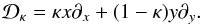 (12)These equations
are analysed in detail in the following sections. For the moment it is instructive to
consider some key properties of the inviscid system.
(12)These equations
are analysed in detail in the following sections. For the moment it is instructive to
consider some key properties of the inviscid system.
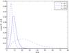 |
Fig. 1 Relaxation to the steady state |

2.3. Time-relaxed inviscid solutions
In the case ν = 0 a steady solution with W = −βZ/α is easily obtained. The form of Z is then constrained by (11) and a description in terms of special functions is possible in special cases (see the axisymmetric solution of Sect. 3.2). More generally, we can determine inviscid solutions computationally – and assess the dynamic accessibility of the solution – by considering the time relaxation of the system (Tassi et al. 2005).
In Fig. 1 we show the recovery of the steady
inviscid solution, from prescribed initial conditions, for three values of
κ. Equations (10) and
(11) were evolved dynamically, using
finite difference replacements, until the system achieved steady state. The plots measure
the modulus of (αW + βZ) at selected times and
demonstrate convergence (to zero) at large t. The simulation assumes the
boundary values 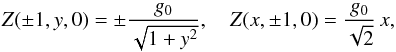 (13)with
Z(x,y,0) = 0 elsewhere, and with
W(x,y,0) = βZ(x,
y,0)/α. These conditions were
chosen to be consistent with the reconnective m = 1 mode described in
Sect. 3.2 and correspond to continuous driving of the
disturbance fields. The parameter g0 controls the strength of
the driving and, for the purposes of obtaining resistive scalings,
g0 is typically adjusted to keep the magnitude of the
magnetic disturbance field | Z| ≃ O(1).
(13)with
Z(x,y,0) = 0 elsewhere, and with
W(x,y,0) = βZ(x,
y,0)/α. These conditions were
chosen to be consistent with the reconnective m = 1 mode described in
Sect. 3.2 and correspond to continuous driving of the
disturbance fields. The parameter g0 controls the strength of
the driving and, for the purposes of obtaining resistive scalings,
g0 is typically adjusted to keep the magnitude of the
magnetic disturbance field | Z| ≃ O(1).
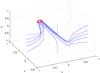 |
Fig. 2 Magnetic field lines at steady state for κ = 0.6, with η = 0.003, ν = 0, α = 1, β = −0.5, g0 = 0.015. |
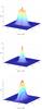 |
Fig. 3 Current density at steady state for different κ values. In the case κ = 0.8 the current layer is quasi-one dimensional and closely aligned to the inflow x-axis. |
The spine structure of the magnetic field lines is shown in Fig. 2 for κ = 0.6. Although, irrespective of κ, the field lines penetrate the fan z = 0 for x > 0, the field lines in the outer field (projected onto the fan) are strictly radial only for κ = 1/2.
This behaviour is reinforced in Fig. 3 which shows the movement away from tube-like current structures for κ ≠ 1/2. For κ > 1/2 in particular, we see that the spine tubes become elongated, leading to more “sheet-like” current structures. Thus κ = 0.8 corresponds closely to current sheet reconnection, in which inflow of oppositely directed field along the x-axis is balanced by outflow along the spine. The inflow switches mainly to the y-axis for κ = 0.2. However, as mentioned in Sect. 3.5 below, this solution has a different character in that the initial conditions (13) no longer guarantee that oppositely directed field lines are driven together by the inflow.
3. Visco-resistive spine reconnection
3.1. The ideal system
To gain analytic insight into the dynamic behaviour of the spine system ((10) and (11)) we first consider the ideal case in which η = ν = 0. We anticipate that singularities in the form of unbounded fields can develop along the spine axis which can only be resolved by resistive effects.
We first observe that the operator
defines a directional derivative along the background field. By changing to the
characteristic coordinates  we
obtain the simplification
we
obtain the simplification  Introducing the comoving frame
  (14)and
eliminating W from the system then yields the Klein-Gordon equation
(14)and
eliminating W from the system then yields the Klein-Gordon equation
 (15)Since an identical
relation may be found for W, this equation holds for any linear
combination of the W and Z disturbances. This
equivalence highlights the inherent symmetry in the v and B
disturbance fields.
(15)Since an identical
relation may be found for W, this equation holds for any linear
combination of the W and Z disturbances. This
equivalence highlights the inherent symmetry in the v and B
disturbance fields.
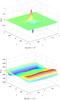 |
Fig. 4 Surface plot of Z field in steady state for | β| < α and | β| > α respectively, illustrating strong localisation of the field in the former case contrasted with an accumulation in the outer field when | β | = α + 0.1. Other parameters are η = 0.001, ν = 0.003, α = 1, κ = 0.5. |
It is interesting that a similar reduction to Klein-Gordon form also occurs for ideal fan reconnection models (Craig & Fabling 1998; Tassi et al. 2005). A key property in all cases is that unbounded exponential growth occurs if α2 > β2. The fastest blow up – as exp(αt) – occurs when β is negligible. In the isotropic case this corresponds to almost straight field lines, washed in radially, developing as a burgeoning flux rope along the spine. However if β2 > α2 Alfvénic wave modes – the incompressible limit of compressive fast modes – can act to disperse the energy in the disturbance field, thwarting the localisation. In this case flow-driven, compressive flux pile-up reconnection cannot occur.
This change in character of the solution for α2 < β2 is unlikely to be undone by the introduction of small resistive and viscous effects. In Fig. 4, for example, we contrast time relaxations with | β| = α/2 and | β| = α + 0.1 keeping all other initial conditions fixed. Well defined solutions are obtained in both cases but the field accumulates in the outer field rather than around the spine for β2 > α2. A similar outer field accumulation occurs for fan solutions when the flow is not sufficiently strong (Craig & Litvinenko 2012).
3.2. The steady axisymmetric solution
Returning to system ((10) and (11)), we now consider the steady resistive
solution for axisymmetric inviscid flow. The relation
W = −βZ(x,y)/α
still holds but, rather than seek a Cartesian representation for
Z(x,y), it is simplest to adopt a polar decomposition
under the assumption of axisymmetry (κ = 1/2). We then
have 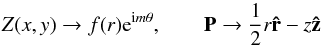 (16)where
r2 = x2 + y2
and tanθ = y/x. The
differential equation for the radial dependence, namely
(16)where
r2 = x2 + y2
and tanθ = y/x. The
differential equation for the radial dependence, namely 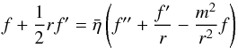 (17)has
a formal solution, assuming f → 0 as r → 0, given by
(17)has
a formal solution, assuming f → 0 as r → 0, given by
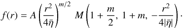 (18)Here A
is a constant and M is a Kummer function with the properties
(18)Here A
is a constant and M is a Kummer function with the properties
 In
these equations
In
these equations  and we must take α > 0 with
α2 > β2
to obtain well behaved spine solutions. All modes have plasma flowing into the fan and
exhausted along the spine (as in Fig. 2).
and we must take α > 0 with
α2 > β2
to obtain well behaved spine solutions. All modes have plasma flowing into the fan and
exhausted along the spine (as in Fig. 2).
Of prime interest is the reconnection mode associated with the spine solution. The mode
m = 0 is exceptional in that the null point is displaced along the
spine axis resulting in a diffuse current, but all other modes (m ≥ 1)
possess fields localised on the scale
rs2 ≃ η that fall off as
1/r2 for large r. The
fact that these behave as rm as
r → 0 shows that the current density, namely ![Mathematical equation: \begin{equation} \vec{J}(r, \theta) = \left[{\rm i} \, m \frac {f(r)} {r} \vec{\hat{r}} - f'(r) \vec{\hat{\theta}} \right] {\rm e}^{{\rm i} m \theta}, \label{jcur} \end{equation}](/articles/aa/full_html/2013/12/aa21815-13/aa21815-13-eq134.png) (19)can be finite at
r = 0 only in the case m = 1. It follows that
m = 1 defines the reconnection mode of the spine solution.
(19)can be finite at
r = 0 only in the case m = 1. It follows that
m = 1 defines the reconnection mode of the spine solution.
3.3. Visco-resistive solutions
With the inclusion of dynamic and viscous effects an exact analytic description is precluded, and solutions must be developed numerically. We follow the time relaxation approach of Sect. 2.3 and adopt the same initial conditions (13). Scaling results are derived by fixing ν while systematically reducing η from 10-2 to 3 × 10⁻⁵. This is repeated for ν = 0.005, 0.003 and 0.001. Since an isotropic background field provides the “purest” spine solution, the value κ = 1/2 will be adopted for the bulk of the numerical simulations in this section.
Our first observation is that, although the inclusion of viscosity causes the relation W = −βZ/α to break down, the qualitative behaviour of the system is largely unaltered. Figure 5, for example, contrasts the relaxation of the inviscid solution with the relaxation for ν = 0.001 and ν = 0.003. Departures from the inviscid relation W = −βZ/α increase with ν but this does not compromise the recovery of a well defined, steady solution.
An important question is whether the inclusion of viscosity influences the scaling of the
spine current tube. Previous studies (e.g. Park et al. 1984) indicate that a hybrid scale could develop that depends on the product
ην. The scaling runs performed below however, suggest that the
axisymmetric, inviscid scale  remains
robust to the inclusion of viscosity even for ν ≫ η.
remains
robust to the inclusion of viscosity even for ν ≫ η.
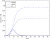 |
Fig. 5 Effect on the steady state relaxation of adding classical viscosity. The ν = 0 curve is identical to that in Fig. 1, with all other parameters kept fixed (η = 0.001, α = 1, β = −0.5, κ = 0.5). |
3.4. Ohmic and viscous dissipation rates
To provide a focus for the numerical results we first make an estimate of the global
Ohmic losses. We make the provisional assumption that the viscosity has only a minor
effect on the scale associated with the localised spine field. In this case
ΔV ≃ πr2 ≃ η
(Craig et al. 1997) and we find that 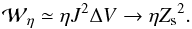 (20)For realistic values
of the collisional resistivity – and with Zs of order unity –
this rate is far too slow to account for flare-like energy release. Even if the
resistivity is enhanced by factors of order 106 due to non-collisional effects,
the resultant dissipation rate
(20)For realistic values
of the collisional resistivity – and with Zs of order unity –
this rate is far too slow to account for flare-like energy release. Even if the
resistivity is enhanced by factors of order 106 due to non-collisional effects,
the resultant dissipation rate  remains several orders of magnitude too small.
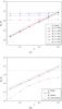 |
Fig. 6 a) Resistive and viscous dissipation as a function of η for three different values of ν (ν = 0.005, 0.003, 0.001). We note that the Ohmic dissipation rates are effectively unchanged despite the differing values of viscosity. b) Resistive and viscous dissipation for ν = 0.003, with the latter separated into contributions from the global background field and the disturbance field. The dotted line indicates η1 scaling in both panels. |
Viscous dissipation can be calculated directly from (9), which in the case of classical viscosity gives 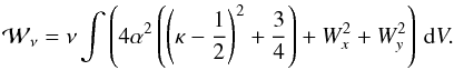 (21)Clearly, the first term
in the integral represents a constant contribution from the non-uniform background flow
required to support the reconnection. For κ ≃ 1/2 this
term yields
(21)Clearly, the first term
in the integral represents a constant contribution from the non-uniform background flow
required to support the reconnection. For κ ≃ 1/2 this
term yields  which gives a power output of around
  in our units (with
α = 1, ∫dV = 4, ν = 10-3).
This output translates to global losses of 1029
erg s
in our units (with
α = 1, ∫dV = 4, ν = 10-3).
This output translates to global losses of 1029
erg s , a
rate which is clearly sufficient to account for a sizable solar flare. However, the
contribution of the reconnection velocity field
, a
rate which is clearly sufficient to account for a sizable solar flare. However, the
contribution of the reconnection velocity field  should
also be taken into account. Since we do not have a sound analytic prediction for this
contribution we must rely on extrapolation of our numerical results.
should
also be taken into account. Since we do not have a sound analytic prediction for this
contribution we must rely on extrapolation of our numerical results.
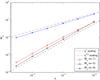 |
Fig. 7 Scalings for different values of κ. As κ increases from 1/2 towards 1 the scaling changes from η to η1/2, as given by Eq. (25). |
Figure 6 shows that our provisional prediction
 is well supported by the numerics. For the three values of viscosity modelled (panel a),
there is little impact on either the scaling of
is well supported by the numerics. For the three values of viscosity modelled (panel a),
there is little impact on either the scaling of  or its magnitude. Our results show that the viscous dissipation
 is dominated by the contribution from the background field, which is proportional to
ν as per Eq. (21).
Specifically, as panel b of Fig. 6 confirms, there is
a rapid fall-off of the reconnective component of the velocity field as η
becomes small. This can be understood by observing that, in steady state, the reconnection
velocity field (10) should scale as
is dominated by the contribution from the background field, which is proportional to
ν as per Eq. (21).
Specifically, as panel b of Fig. 6 confirms, there is
a rapid fall-off of the reconnective component of the velocity field as η
becomes small. This can be understood by observing that, in steady state, the reconnection
velocity field (10) should scale as
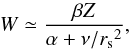 (22)where
rs is the radial extent of the spine current tube. Taking
rs2 ≃ η then implies
W ~ η provided that
ν ≫ η.
(22)where
rs is the radial extent of the spine current tube. Taking
rs2 ≃ η then implies
W ~ η provided that
ν ≫ η.
We conclude that, as far as the global energy losses are concerned, the spine current layer provides the main contribution from the magnetic field (~η) whereas the global flow accounts for the bulk of the viscous dissipation (~ν). The fact that ν ≫ η therefore implies that strong damping of the velocity field can occur even in the presence of very weak reconnection rates.
3.5. Breakdown of axisymmetry
The previous results apply to strictly axisymmetric background fields. When
κ ≠ 1/2, the amplitude of background viscous
dissipation is altered slightly, but the overall scaling
 is unaffected (see Eq. (21)). The rates
for
is unaffected (see Eq. (21)). The rates
for  do, however, vary markedly with κ, as illustrated in Fig. 7. In particular as κ → 1 we recover the
current sheet scaling
do, however, vary markedly with κ, as illustrated in Fig. 7. In particular as κ → 1 we recover the
current sheet scaling  .
The lack of symmetry about κ = 1/2, perhaps surprising
at first sight, can be viewed as an artefact of the initial/boundary conditions since only
κ = 1 corresponds to anti-parallel merging. The limit
κ = 0 is essentially a non-reconnective mode, in which like (as opposed
to oppositely directed) fields are driven together. For this reason we concentrate on the
range 1/2 ≤ κ ≤ 1 when developing reconnection scaling
laws.
.
The lack of symmetry about κ = 1/2, perhaps surprising
at first sight, can be viewed as an artefact of the initial/boundary conditions since only
κ = 1 corresponds to anti-parallel merging. The limit
κ = 0 is essentially a non-reconnective mode, in which like (as opposed
to oppositely directed) fields are driven together. For this reason we concentrate on the
range 1/2 ≤ κ ≤ 1 when developing reconnection scaling
laws.
In the regime
1/2 < κ < 1
with ν ≫ η, it is straightforward to make the estimate
 (23)based on the
resistive scale
(23)based on the
resistive scale  and the
geometric scaling
ΔV ≃ η1/2κ
(e.g. Craig et al. 1997). This result correctly
interpolates between the current sheet (κ = 1) and the spine reconnection
(κ = 1/2) data.
and the
geometric scaling
ΔV ≃ η1/2κ
(e.g. Craig et al. 1997). This result correctly
interpolates between the current sheet (κ = 1) and the spine reconnection
(κ = 1/2) data.
3.6. Role of the Braginskii viscosity
In general the Braginskii viscosity tensor cannot be incorporated within the analytic spine treatment (8). Since the spine reduction remains valid, however, in the special case β = 0, we can argue by physical continuity, that this limit should approximate the behaviour of the system for sufficiently small β. A more general treatment probably requires a fully 3D numerical formulation, which we do not pursue here.
In the case β = 0 the background field is absent and so
B = Z(x,y,t)ẑ. Equation
(6) now allows a direct calculation of
the viscous dissipation  (24)Since
ν0 ≃ ν we see that Braginskii dissipation
is only marginally less effective than the classical losses (21). The implication is that both models of viscosity are capable of
providing physically significant damping of the non-uniform velocity fields associated
with reconnection.
(24)Since
ν0 ≃ ν we see that Braginskii dissipation
is only marginally less effective than the classical losses (21). The implication is that both models of viscosity are capable of
providing physically significant damping of the non-uniform velocity fields associated
with reconnection.
4. Discussion and conclusions
We have considered 3D visco-resistive spine reconnection for both the classical and
Braginskii forms of the fluid viscosity. Steady reconnection solutions were obtained by time
relaxation of the governing MHD equations. Although viscosity was found to be ineffective at
dissipating energy on the small resistive scale  ,
it did provide effective damping on the global scale of the non-uniform flow that supports
the reconnection. While this might eventually be expected to slow the flow enough to stall
the reconnection, the associated power output
,
it did provide effective damping on the global scale of the non-uniform flow that supports
the reconnection. While this might eventually be expected to slow the flow enough to stall
the reconnection, the associated power output  is still small compared with the background kinetic energy which is of order unity. We
expect therefore that realistic levels of viscous damping will allow the flow to remain
strong enough to localise the field while still providing significant levels of viscous
dissipation. This conclusion is consistent with recent dynamic reconnection studies in which
the current localisation is driven by the Orzag-Tang vortex (Armstrong & Craig 2013).
is still small compared with the background kinetic energy which is of order unity. We
expect therefore that realistic levels of viscous damping will allow the flow to remain
strong enough to localise the field while still providing significant levels of viscous
dissipation. This conclusion is consistent with recent dynamic reconnection studies in which
the current localisation is driven by the Orzag-Tang vortex (Armstrong & Craig 2013).
More specifically, we showed that the ratio of the global viscous losses to the Ohmic
losses satisfied  (25)where
1/2 ≤ κ ≤ 1 depends on the isotropy of the merging.
(25)where
1/2 ≤ κ ≤ 1 depends on the isotropy of the merging.
The scaling for κ ≃ 1/2 in which
 is a new result that derives from the tubular current structures of axisymmetric spine
reconnection. This result strengthens previous findings that slow reconnective merging can
be associated with flare-like rates of viscous energy dissipation. Yet even for current
sheet models where the weaker relation with κ ≃ 1 holds, global viscous
losses should still dominate resistive losses localised to the current layer by several
orders of magnitude. This dominance is independent of whether classical or Braginskii
viscosity is employed and probably holds good even if the collisional resistivity is
enhanced through turbulent effects by factors approaching one million.
is a new result that derives from the tubular current structures of axisymmetric spine
reconnection. This result strengthens previous findings that slow reconnective merging can
be associated with flare-like rates of viscous energy dissipation. Yet even for current
sheet models where the weaker relation with κ ≃ 1 holds, global viscous
losses should still dominate resistive losses localised to the current layer by several
orders of magnitude. This dominance is independent of whether classical or Braginskii
viscosity is employed and probably holds good even if the collisional resistivity is
enhanced through turbulent effects by factors approaching one million.
It is interesting that the present analysis seems to preclude to the development of a
hybrid, visco-resistive scale, typically of the form  (Park et al. 1984). Models of transient
X-point collapse in closed, line-tied, geometries, for instance, are
known to develop hybrid scales that significantly weaken the global energy release, in
apparent contradiction to the present study (Craig et al. 2005). Such weak rates of energy release, however, emerge only after an initial
transient phase in which a significant fraction of the excess X-point
energy is viscously dissipated. It seems likely therefore that viscous losses could dominate
resistive losses for a wide range of reconnection geometries.
(Park et al. 1984). Models of transient
X-point collapse in closed, line-tied, geometries, for instance, are
known to develop hybrid scales that significantly weaken the global energy release, in
apparent contradiction to the present study (Craig et al. 2005). Such weak rates of energy release, however, emerge only after an initial
transient phase in which a significant fraction of the excess X-point
energy is viscously dissipated. It seems likely therefore that viscous losses could dominate
resistive losses for a wide range of reconnection geometries.
Acknowledgments
We would like to thank Yuri Litvinenko and Craig Armstrong for several helpful comments.
References
- Armstrong, C. K., & Craig, I. J. D. 2013, Sol. Phys., 283, 463 [NASA ADS] [CrossRef] [Google Scholar]
- Armstrong, C. K., Craig, I. J. D., & Litvinenko, Y. E. 2012, ApJ, 767, 165 [NASA ADS] [CrossRef] [Google Scholar]
- Braginskii, S. I. 1965, Rev. Plasma Phys., 1, 205 [NASA ADS] [Google Scholar]
- Cassak, P. A., Drake, J. F., & Shay, M. A. 2006, ApJ, 644, L145 [NASA ADS] [CrossRef] [Google Scholar]
- Craig, I. J. D., & Fabling, R. B. 1996, ApJ, 462, 969 [NASA ADS] [CrossRef] [Google Scholar]
- Craig, I. J. D., & Fabling, R. B. 1998, Phys. Plasmas, 5, 635 [NASA ADS] [CrossRef] [Google Scholar]
- Craig, I. J. D., & Litvinenko, Y. E. 2012, ApJ, 747, 16 [NASA ADS] [CrossRef] [Google Scholar]
- Craig, I. J. D., Fabling, R. B., & Watson, P. G. 1997, ApJ, 485, 383 [NASA ADS] [CrossRef] [Google Scholar]
- Craig, I. J. D., Litvinenko, Y. E., & Senanayake, T. 2005, A&A, 433, 1139 [NASA ADS] [CrossRef] [EDP Sciences] [Google Scholar]
- Heerikhuisen, J., Litvinkenko, Y. E., & Craig, I. J. D. 2002, ApJ, 566, 512 [NASA ADS] [CrossRef] [Google Scholar]
- Hollweg, J. V. 1986, ApJ, 306, 730 [NASA ADS] [CrossRef] [Google Scholar]
- Hosking, R. J., & Marinoff, G. M. 1973, Plasma Phys., 15, 327 [NASA ADS] [CrossRef] [Google Scholar]
- Kowal, G., Lazarian, A., Vishniac, E. T., & Otmianowska-Mazur, K. 2009, ApJ, 700, 63 [NASA ADS] [CrossRef] [Google Scholar]
- Lau, Y. T., & Finn, J. M. 1990, ApJ, 350, 672 [NASA ADS] [CrossRef] [Google Scholar]
- Litvinenko, Y. E. 2005, Sol. Phys., 229, 203 [NASA ADS] [CrossRef] [Google Scholar]
- Litvinenko, Y. E. 2006, A&A, 452, 1069 [NASA ADS] [CrossRef] [EDP Sciences] [Google Scholar]
- Park, W., Monticello, D. A., & White, R. B. 1984, Phys. Fluids, 27, 137 [NASA ADS] [CrossRef] [Google Scholar]
- Priest, E. R., & Forbes, T. 2000, Magnetic reconnection: MHD theory and applications (Cambridge Univ. Press) [Google Scholar]
- Priest, E. R., & Titov, V. S. 1996, Roy. Soc. London. Philos. Trans. Ser. A, 354, 2951 [Google Scholar]
- Somov, B.V., & Titov, V. S. 1983, Sov. Astron. Lett., 9, 26 [NASA ADS] [Google Scholar]
- Sonnerup, B. U. O., & Priest, E. R. 1975, J. Plasma Phys., 14, 283 [NASA ADS] [CrossRef] [Google Scholar]
- Spitzer, L. 1962, Physics of fully ionized gases (NewYork-London: Interscience Publishing) [Google Scholar]
- Stanier, A., Browning, P., & Dalla, S. 2012, A&A, 542, A47 [NASA ADS] [CrossRef] [EDP Sciences] [Google Scholar]
- Tassi, E., Titov, V. S., & Hornig, G., 2005, Phys. Plasmas, 12, 112902 [NASA ADS] [CrossRef] [Google Scholar]
- Titov, V. S., & Priest, E. R. 1997, J. Fluid Mech., 348, 327 [NASA ADS] [CrossRef] [Google Scholar]
- Wyper, P. F., & Pontin, D. I. 2013, Phys. Plasmas, 20, 032117 [NASA ADS] [CrossRef] [Google Scholar]
All Figures
|
Fig. 1 Relaxation to the steady state |
| In the text | |
|
Fig. 2 Magnetic field lines at steady state for κ = 0.6, with η = 0.003, ν = 0, α = 1, β = −0.5, g0 = 0.015. |
| In the text | |
|
Fig. 3 Current density at steady state for different κ values. In the case κ = 0.8 the current layer is quasi-one dimensional and closely aligned to the inflow x-axis. |
| In the text | |
|
Fig. 4 Surface plot of Z field in steady state for | β| < α and | β| > α respectively, illustrating strong localisation of the field in the former case contrasted with an accumulation in the outer field when | β | = α + 0.1. Other parameters are η = 0.001, ν = 0.003, α = 1, κ = 0.5. |
| In the text | |
|
Fig. 5 Effect on the steady state relaxation of adding classical viscosity. The ν = 0 curve is identical to that in Fig. 1, with all other parameters kept fixed (η = 0.001, α = 1, β = −0.5, κ = 0.5). |
| In the text | |
|
Fig. 6 a) Resistive and viscous dissipation as a function of η for three different values of ν (ν = 0.005, 0.003, 0.001). We note that the Ohmic dissipation rates are effectively unchanged despite the differing values of viscosity. b) Resistive and viscous dissipation for ν = 0.003, with the latter separated into contributions from the global background field and the disturbance field. The dotted line indicates η1 scaling in both panels. |
| In the text | |
|
Fig. 7 Scalings for different values of κ. As κ increases from 1/2 towards 1 the scaling changes from η to η1/2, as given by Eq. (25). |
| In the text | |
Current usage metrics show cumulative count of Article Views (full-text article views including HTML views, PDF and ePub downloads, according to the available data) and Abstracts Views on Vision4Press platform.
Data correspond to usage on the plateform after 2015. The current usage metrics is available 48-96 hours after online publication and is updated daily on week days.
Initial download of the metrics may take a while.