| Issue |
A&A
Volume 555, July 2013
|
|
|---|---|---|
| Article Number | A27 | |
| Number of page(s) | 9 | |
| Section | The Sun | |
| DOI | https://doi.org/10.1051/0004-6361/201220195 | |
| Published online | 24 June 2013 | |
Damping of coronal loop kink oscillations due to mode conversion⋆
1
Solar Physics and Space Plasma Research Centre
(SP 2RC), University of Sheffield,
Hicks Building, Hounsfield Road,
Sheffield
S3 7RH,
UK
e-mail: This email address is being protected from spambots. You need JavaScript enabled to view it.
2
Departament de Física, Universitat de les Illes
Balears, 07122
Palma de Mallorca,
Spain
Received:
9
August
2012
Accepted:
24
April
2013
Abstract
The damping of kink oscillations of a thin magnetic tube due to mode conversion, also called resonant absorption, is studied. The tube consists of a homogeneous core region and an inhomogeneous annulus, where the density monotonically decreases from its value in the core region to the value in the surrounding plasma. The annulus is assumed to be thin, so the study is carried out in the thin tube thin boundary approximation. The equation governing the amplitude variation of kink oscillations is derived. The initial value problem for this equation is solved to study the resonant damping. This means that, in particular, we study the transient state before the loop oscillates with the stationary or nearly stationary state. The results are compared with those of the direct numerical modelling, and the agreement is found to be fairly good. On the basis of the solution to the initial value problem for the governing equation, the damping time is calculated and compared with that given by the classical theory of resonant absorption. It is found that the classical theory underestimates the damping time, with the error increasing with the increase of the annulus thickness. However, the error is not large, so the damping time given by the classical theory of resonant absorption can be taken as a sufficiently good approximation.
Key words: magnetohydrodynamics (MHD) / Sun: corona / Sun: oscillations
Appendix A is available in electronic form at http://www.aanda.org
© ESO, 2013
1. Introduction
After coronal loop kink oscillations were first observed by Transition Region and Coronal Explorer (TRACE) in 1998 and reported by Aschwanden et al. (1999) and Nakariakov et al. (1999), they remain in the limelight of solar physics. One important property of these oscillations is that they are heavily damped with the damping time of the order of a few oscillation periods. A few mechanisms of this damping were suggested. At present the most reliable and comprehensively studied damping mechanism is resonant absorption that is related to the conversion of a global kink oscillation into local small-scale Alfvénic oscillations. Resonant absorption was suggested as a possible mechanism of damping of (at that time hypothetical) coronal loop kink oscillations by Hollweg & Yang (1988). Later it was more comprehensively studied by Goossens et al. (1992). Ruderman & Roberts (2002) studied the first observed event and found that resonant absorption is a viable mechanism of damping of coronal loop kink oscillations. Later Goossens et al. (2002) applied it to 12 events of coronal loop oscillations reported by Ofman & Aschwanden (2002) and confirmed the conclusion made by Ruderman & Roberts (2002).
Following earlier studies (see, e.g. Sedláček 1971) of resonant absorption, Hollweg & Yang (1988) used the ideal magnetohydrodynamic (MHD) equations to describe the resonant damping of kink oscillations. In this approach the damping occurs due to the singularity on the Riemann surface of the Laplace transform of the solution when it is extended from the principal sheet to the non-principal sheets of the Riemann surface. Although this approach is mathematically perfectly correct, the occurrence of damping looks like a mathematical trick because all physical processes at the vicinity of the resonant surface are ignored.
Goossens et al. (1992) adopted another approach based on the use of dissipative MHD for the description of wave motion in the vicinity of the resonant surface. To calculate the decrement, they used the connection formulae first introduced by Sakurai et al. (1991). The idea of this approach is the following. Dissipation is important only in a thin dissipative layer embracing the resonant surface because it is characterised by large gradients. The plasma motion can be described by the ideal MHD outside the dissipative layer. The solution of the dissipative MHD equations is used to calculate the jumps of the total pressure and the normal velocity component across the dissipative layer. The magnitudes of these jumps are given by the connection formulae. They are used to connect the ideal MHD solutions at the two sides of the dissipative layer. Sakurai et al. (1991) presented the solution of the dissipative MHD equations in the dissipative layer in terms of Bessel functions. Later Goossens et al. (1995) improved the analysis by Sakurai et al. (1991) and expressed the solution in the dissipative layer in a much simpler form in terms of the so-called F and G functions.
The connection formulae were first used to study the resonant absorption in the driven problem, where the steady state of oscillation is created by an external harmonic driver. Later Goossens et al. (1992) used them to study the damping of viscous eigenmodes in cylindrical geometry. In fact, a similar approach based on matching the ideal MHD solution outside the dissipative layer with the dissipative MHD solution inside it was used by Mok & Einaudi (1985) to study the damping of surface waves propagating along a transitional layer between two homogeneous regions, although these authors did not introduce the connection formulae explicitly.
Mok & Einaudi (1985) were probably the first
who pointed out that the solution in the dissipative layer obtained for the driven problem
can be used to describe the eigenmodes of dissipative MHD only when the dissipation is
strong enough. To formulate this condition explicitly, we first need to specify the
equilibrium. In what follows we consider a straight magnetic tube of
radius R and length L ≫ R. In
cylindrical coordinates r, ϕ, z the
plasma density is given by  (1)where
ρi and ρe are constants,
ρi > ρe,
and ρt(r) is a monotonically decreasing
function, ρt(R − ℓ/2) = ρi,
ρt(R + ℓ/2) = ρe.
We also assume that the transitional layer is thin, ℓ ≪ R.
Hence, we use the thin tube thin boundary (TTTB) approximation. We also use the
approximation of cold plasma relevant for the coronal conditions.
(1)where
ρi and ρe are constants,
ρi > ρe,
and ρt(r) is a monotonically decreasing
function, ρt(R − ℓ/2) = ρi,
ρt(R + ℓ/2) = ρe.
We also assume that the transitional layer is thin, ℓ ≪ R.
Hence, we use the thin tube thin boundary (TTTB) approximation. We also use the
approximation of cold plasma relevant for the coronal conditions.
In the viscous and magnetic Reynolds numbers,
Re = Ckℓ/ν
and Rm = Ckℓ/λ,
ν is the shear kinematic viscosity, λ is the magnetic
diffusion coefficient, and Ck is the kink speed determined by
 (2)where B
is the magnitude of the (constant) equilibrium magnetic field
and μ0 the magnetic permeability of free space. To
characterise the simultaneous effect of viscosity and resistivity, we introduce the total
Reynolds number Rt defined by
(2)where B
is the magnitude of the (constant) equilibrium magnetic field
and μ0 the magnetic permeability of free space. To
characterise the simultaneous effect of viscosity and resistivity, we introduce the total
Reynolds number Rt defined by  (3)Then
the condition that dissipation is strong enough to ensure that the solution in the
dissipative layer obtained for the driven problem can be used to describe the eigenmodes of
dissipative MHD is written as (e.g. Ruderman et al.
1995)
(3)Then
the condition that dissipation is strong enough to ensure that the solution in the
dissipative layer obtained for the driven problem can be used to describe the eigenmodes of
dissipative MHD is written as (e.g. Ruderman et al.
1995)  (4)Ruderman et al. (1995) reconsidered the problem studied
by Mok & Einaudi (1985) when this condition
is not satisfied. They showed that, while the solution describing the plasma motion in the
dissipative layer is very much different from that obtained for the driven problem, the
damping rate of the surface mode remains the same. Later Tirry & Goossens (1996) extended this analysis to the cylindrical geometry
(see also the review paper by Goossens et al. 2011).
They expressed the solution in the dissipative layer in terms
of FΛ and GΛ functions, which are
the generalisation of F and G functions and coincide with
these functions when Λ = 0. Using this solution they showed that the connection formulae
remain the same, even when the condition (4)
is not satisfied. We note that for typical conditions in the solar
corona Rt ≳ (L/ℓ)4.
(4)Ruderman et al. (1995) reconsidered the problem studied
by Mok & Einaudi (1985) when this condition
is not satisfied. They showed that, while the solution describing the plasma motion in the
dissipative layer is very much different from that obtained for the driven problem, the
damping rate of the surface mode remains the same. Later Tirry & Goossens (1996) extended this analysis to the cylindrical geometry
(see also the review paper by Goossens et al. 2011).
They expressed the solution in the dissipative layer in terms
of FΛ and GΛ functions, which are
the generalisation of F and G functions and coincide with
these functions when Λ = 0. Using this solution they showed that the connection formulae
remain the same, even when the condition (4)
is not satisfied. We note that for typical conditions in the solar
corona Rt ≳ (L/ℓ)4.
While the use of connection formulae is perfectly correct when studying the driven problem,
their application to the initial value problem is doubtful. The point is that the derivation
of connection formulae for the initial value problem is based on the assumption that the
plasma motion near the ideal resonant position is described by
the FΛ and GΛ functions. To be
specific, we consider the coronal loop kink oscillations. It was shown by Ruderman & Roberts (2002) that, under not very
restrictive assumptions about the initial conditions, the fundamental kink mode of the
coronal loop kink oscillation emerges from the initial perturbation after the transitional
time of the order of one oscillation period (see also the numerical work by Terradas et al. 2006). However, the plasma motion in this
oscillation is described fairly well by the eigenmode of dissipative MHD only far from the
resonant surface. Near the resonant surface, the plasma motion is approximately described by
the dissipative eigenmode only when the spatial scales of the order
of  have been formed. This occurs
after the transitional time of the order of
have been formed. This occurs
after the transitional time of the order of  times the oscillation period (e.g. Kappraff &
Tataronis 1977; Poedts et al. 1990; Mann et al. 1995). For typical coronal conditions we
have Re ~ Rm, so for the estimates
we can take Rt ~ Rm. For the
coefficient of magnetic diffusion, we
have λ = 109 T−3/2m2 s-1
(e.g. Priest 1982). Then,
taking Ck = 1000 km s-1
and ℓ = 1000km we obtain Rm = 1010,
and we can take
times the oscillation period (e.g. Kappraff &
Tataronis 1977; Poedts et al. 1990; Mann et al. 1995). For typical coronal conditions we
have Re ~ Rm, so for the estimates
we can take Rt ~ Rm. For the
coefficient of magnetic diffusion, we
have λ = 109 T−3/2m2 s-1
(e.g. Priest 1982). Then,
taking Ck = 1000 km s-1
and ℓ = 1000km we obtain Rm = 1010,
and we can take  as a typical value.
Hence, the time needed for the formation of spatial scales of the order
of is about 1000 oscillation
periods. At that time we can expect the spatial scale of the order of 1 km. On the other
hand, observations show that the damping of coronal loop kink oscillations occurs after a
few oscillation periods. At that time scale, the plasma motion near the resonant surface is
quite different from that described by FΛ
and GΛ functions. This means that the main assumption made by
Ruderman et al. (1995) and Tirry & Goossens (1996) when deriving the connection fortmulae is
not satisfied.
as a typical value.
Hence, the time needed for the formation of spatial scales of the order
of is about 1000 oscillation
periods. At that time we can expect the spatial scale of the order of 1 km. On the other
hand, observations show that the damping of coronal loop kink oscillations occurs after a
few oscillation periods. At that time scale, the plasma motion near the resonant surface is
quite different from that described by FΛ
and GΛ functions. This means that the main assumption made by
Ruderman et al. (1995) and Tirry & Goossens (1996) when deriving the connection fortmulae is
not satisfied.
Recently, the problem of spatial resonant damping of kink waves excited by a driver at the footpoint of a semi-infinite magnetic tube and then propagating along this tube has attracted the attention of solar physicists (Ruderman et al. 2010; Terradas et al. 2010; Soler et al. 2011). In particular, it was shown with the use of connection formulae that in the linear approximation the waves damp exponentially with the distance from the driver, and the damping length has been calculated. The same problem has been studied numerically by Pascoe et al. (2010, 2011, 2012). In particular, Pascoe et al. (2012) have shown that the wave amplitude does not decay exponentially everywhere. At distances of the order of a few wave lengths, the amplitude dependence on the distance is described by the Gaussian profile. At larger distances the amplitude decays exponentially. Motivated by these results, Hood et al. (2013) developed the analytic theory of spatial wave damping that matches very well the results of numerical modelling.
There is a very close similarity between the spatial resonant damping of propagating kink waves and temporal damping of standing kink waves. Hence, we can expect that purely exponential damping does not describe properly the time dependence of the amplitude of kink oscillations. The aim of this paper is to study this problem analytically and then compare the results with the direct numerical modelling. The paper is organised as follows. In the next section we formulate the problem and present the governing equations, as well as the initial and boundary conditions. In Sect. 3 we derive the equation that describes the variation of the kink oscillation amplitude. In Sect. 4 we use this equation to study the damping of kink oscillations due to resonant absorption. Section 5 contains the summary of the results and our conclusions.
2. Problem formulation and governing equations
In our analysis we use the equation derived by Ruderman (2011, hereafter Paper I). This is
Eq. (23) in Paper I, with its right-hand side given by Eq. (24). This equation describes
kink oscillations of a straight magnetic tube in the thin tube approximation in cold plasma
in the presence of background flow. The tube consists of a core region, whose density does
not vary in the radial direction and an annulus surrounding this region, where the density
monotonically changes from its value in the core region to its value in the surrounding
plasma. If we assume that there is no background, flow then Eq. (23) of Paper I reduces to
 (5)Here η
is the radial displacement in the core region, where it is independent of r
in cylindrical coordinates r, ϕ, z, with
the z-axis coinciding with the loop axis; ρ is the
equilibrium plasma density given by Eq. (1),
and Ck is the kink speed given by Eq. (2). The right-hand side of Eq. (5) describes the wave damping due to resonant
absorption. The quantity
(5)Here η
is the radial displacement in the core region, where it is independent of r
in cylindrical coordinates r, ϕ, z, with
the z-axis coinciding with the loop axis; ρ is the
equilibrium plasma density given by Eq. (1),
and Ck is the kink speed given by Eq. (2). The right-hand side of Eq. (5) describes the wave damping due to resonant
absorption. The quantity  is given by
  (6)where P = Bbz/μ0
is the magnetic pressure perturbation, bz is
the z-component of the magnetic field
perturbation, ξr
and ξϕ are the plasma displacements in the
radial and azimuthal direction, δP
and δξr are the jumps
of P and ξr across the
annulus, and VA is the Alfvén speed determined by
(6)where P = Bbz/μ0
is the magnetic pressure perturbation, bz is
the z-component of the magnetic field
perturbation, ξr
and ξϕ are the plasma displacements in the
radial and azimuthal direction, δP
and δξr are the jumps
of P and ξr across the
annulus, and VA is the Alfvén speed determined by  (7)We
note that ξr = η
for r ≤ R − ℓ/2. As
we have already stated, in the following we use the TTTB approximation and assume that the
annulus is
thin, ϵ = ℓ/R ≪ 1.
In accordance with this, we will calculate
only in the leading order approximation with respect to ϵ.
(7)We
note that ξr = η
for r ≤ R − ℓ/2. As
we have already stated, in the following we use the TTTB approximation and assume that the
annulus is
thin, ϵ = ℓ/R ≪ 1.
In accordance with this, we will calculate
only in the leading order approximation with respect to ϵ.
In Paper I the equations describing the plasma motion in terms of the magnetic pressure
perturbation P and the plasma
displacement ξ are derived (see Eqs. (11) and (12)). It is
also pointed out in the paragraph before Eq. (48) in Paper I that the ratio of the left-hand
side of Eq. (11) to its right-hand side is  ,
so that the right-hand side can be neglected in the thin tube approximation. We would like
to study linearly polarised kink oscillations. In accordance with this we
take ξr ∝ cosϕ, P ∝ cosϕ,
and ξϕ ∝ −sinϕ. Then
Eq. (11) of Paper I with the left-hand side equal to zero and Eq. (12)
with U = 0 (no equilibrium flow) reduce to
,
so that the right-hand side can be neglected in the thin tube approximation. We would like
to study linearly polarised kink oscillations. In accordance with this we
take ξr ∝ cosϕ, P ∝ cosϕ,
and ξϕ ∝ −sinϕ. Then
Eq. (11) of Paper I with the left-hand side equal to zero and Eq. (12)
with U = 0 (no equilibrium flow) reduce to  We
assume that the magnetic field lines are frozen in the dense photospheric plasma at the loop
footpoints. Hence, we impose the boundary conditions
We
assume that the magnetic field lines are frozen in the dense photospheric plasma at the loop
footpoints. Hence, we impose the boundary conditions  (11)In
what follows we restrict our attention to the fundamental mode of kink oscillations and
take η, ξr,
ξϕ, and P proportional
to sin(kz),
where k = π/L.
(11)In
what follows we restrict our attention to the fundamental mode of kink oscillations and
take η, ξr,
ξϕ, and P proportional
to sin(kz),
where k = π/L.
As we have already mentioned, the motion far from the Alfvén resonant surface, in
particular, the motion outside the inhomogeneous annulus, is described fairly well by the
eigenmode after the transitional time of the order of the oscillation period. Hence, after
this transitional time, the plasma motion is the harmonic oscillation with the
frequency ω = kCk and the
amplitude slowly decaying due to resonant absorption. This implies that we can use the
approximate relation  (12)which
is valid for η, ξr,
and δξr. However, this is
generally not true for the variation of ξϕ
inside the inhomogeneous layer. Using the prescribed dependence on z and
Eq. (12), we rewrite Eqs. (5), (6), (9), and (10) as
(12)which
is valid for η, ξr,
and δξr. However, this is
generally not true for the variation of ξϕ
inside the inhomogeneous layer. Using the prescribed dependence on z and
Eq. (12), we rewrite Eqs. (5), (6), (9), and (10) as 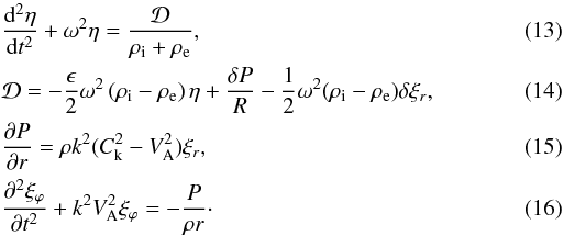 Equation (8) does not change.
We also need to impose the initial conditions. We assume that at the initial moment of time
the loop is pushed by an external pulse to oscillate with the fundamental frequency. This
implies, in particular, that the initial conditions for η are 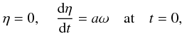 (17)where a
is a positive constant. In the homogeneous
core ξϕ = η,
so ∂ξϕ/∂t = aω
at t = 0. Outside the inhomogeneous layer
(r > R + ℓ/2) ξϕ =−η/r2.
We assume that in the inhomogeneous transitional layer
(17)where a
is a positive constant. In the homogeneous
core ξϕ = η,
so ∂ξϕ/∂t = aω
at t = 0. Outside the inhomogeneous layer
(r > R + ℓ/2) ξϕ =−η/r2.
We assume that in the inhomogeneous transitional layer 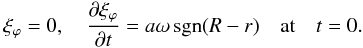 (18)Equations (13)–(16), together with the initial conditions (17) and (18), will be
used in the next section to derive the equation for η.
(18)Equations (13)–(16), together with the initial conditions (17) and (18), will be
used in the next section to derive the equation for η.
3. Derivation of the governing equation for η
In order to derive the governing equation for η, we need to
express
in terms of η. As we have already mentioned, in the homogeneous
core ξr is independent of r,
so ξr = η
for r ≤ R − ℓ/2. It
is shown in Paper I (see Eq. (17)) that P is a linear homogeneous function
of r and  (see the paragraph before Eq. (20) in Paper I). Then it follows from Eq. (15) that
 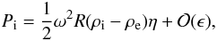 (19)where Pi = P
at r = R − ℓ/2. It
also follows from Eq. (17) of Paper I that
(19)where Pi = P
at r = R − ℓ/2. It
also follows from Eq. (17) of Paper I that  (20)Using
Eqs. (19) and (20), we can see that the first and second term
in Eq. (14) cancel each other.
(20)Using
Eqs. (19) and (20), we can see that the first and second term
in Eq. (14) cancel each other.
The next step is to
express δξr in terms
of η. For this we first need to solve Eq. (16) with respect to ξϕ.
Using Eqs. (19) and (20), we rewrite Eq. (16) in the approximate form valid in the
inhomogeneous annulus,  (21)The
solution to this equation satisfying the initial conditions (18) is
(21)The
solution to this equation satisfying the initial conditions (18) is  (22)where
 (23)In
what follows we also assume that the density profile in the inhomogeneous layer is linear,
so
(23)In
what follows we also assume that the density profile in the inhomogeneous layer is linear,
so ![Mathematical equation: \begin{eqnarray} \rho_{\rm t}(r) = \frac1\ell[\rho_{\rm i}(R+\ell/2-r) - \rho_{\rm e}(R-\ell/2 -r)]. \label{eq:3.6} \end{eqnarray}](/articles/aa/full_html/2013/07/aa20195-12/aa20195-12-eq90.png) (24)Using
Eqs. (8) and (22), we then obtain
(24)Using
Eqs. (8) and (22), we then obtain  (25)where
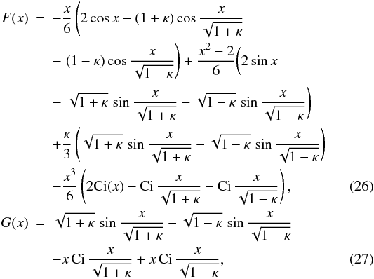 and Ci(x)
is the integral cosine defined by
and Ci(x)
is the integral cosine defined by 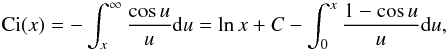 (28)with C ≈ 0.5772
being the Euler constant. Using Eq. (25), we
can express
in terms of η. Substituting the obtained result in Eq. (13), we eventually arrive at the governing
equation for η,
(28)with C ≈ 0.5772
being the Euler constant. Using Eq. (25), we
can express
in terms of η. Substituting the obtained result in Eq. (13), we eventually arrive at the governing
equation for η, 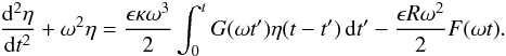 (29)This
integro-differential equation describes the evolution of the tube displacement with time. In
the next section it will be used to study resonant damping of kink oscillations.
(29)This
integro-differential equation describes the evolution of the tube displacement with time. In
the next section it will be used to study resonant damping of kink oscillations.
4. Resonant damping of kink oscillations
First we discuss the asymptotic behaviour of the solution to Eq. (29) for large t. It follows
from Eq. (
A.23) in Appendix A that
for πϵωt/8 ~ 1 the oscillation amplitude is
proportional to e−γdt,
where 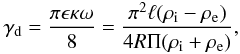 (30)and Π = 2π/ω
is the wave period. This is a familiar result (see, e.g. Goossens et al. 1992, 2002; Ruderman &
Roberts 2002). We have imposed the
restriction πϵωt/8 ~ 1 and do not consider a larger
time, ωt ≫ ϵ-1, because in accordance with
Eq. (A.23) Eq. (29) describes the exponential decay of
oscillation amplitude only for t ~ 8(πϵω)-1.
For ωt ≫ ϵ-1, the
term
(30)and Π = 2π/ω
is the wave period. This is a familiar result (see, e.g. Goossens et al. 1992, 2002; Ruderman &
Roberts 2002). We have imposed the
restriction πϵωt/8 ~ 1 and do not consider a larger
time, ωt ≫ ϵ-1, because in accordance with
Eq. (A.23) Eq. (29) describes the exponential decay of
oscillation amplitude only for t ~ 8(πϵω)-1.
For ωt ≫ ϵ-1, the
term  on the right-hand side of Eq. (A.23) is
either comparable with the exponential term or even dominant. Hence, it seems that
Eq. (29) is valid only
for πϵωt/8 ≲ 1.
on the right-hand side of Eq. (A.23) is
either comparable with the exponential term or even dominant. Hence, it seems that
Eq. (29) is valid only
for πϵωt/8 ≲ 1.
Equation (A.11) expresses the solution of Eq. (29) in terms of integral along the real axis. It can be used to study the dependence of η on time. However, we preferred to solve Eq. (29) numerically. To do this we approximated the derivative on the left-hand side of this equation by the central difference and used the trapezoid rule to calculate the integral on the right-hand side. As a complementary analysis we have also solved the problem numerically by using the original linearised MHD equations and applying the initial conditions given by Eqs. (17), (18) (see Terradas et al. 2006, for further details). This allows us to compare the performance of the two methods. The results of the numerical solution of Eq. (29) and the direct numerical modelling for various values of ϵ are shown in Fig. 1–6. In all calculations we took ζ = ρi/ρe = 3, so that κ = 1/2. Figures 1–3 show the solution of Eq. (29), together with solutions obtained by the direct numerical modelling for ϵ = 0.1, 0.2, 0.3. In what follows we define the damping time td as the time when the oscillation amplitude decreases e times in comparison with its initial value. In Figs. 1–3 the solutions are shown on the time interval approximately equal to 2td. We note that, while the solid and dashed curve in each figure practically coincide for first few periods, the amplitude of the solid curve becomes slightly smaller than that of the dashed curve for large time. We attribute this difference to the approximations made in the derivation of Eq. (29). This comparison gives further support to the conclusion that Eq. (29) is valid only for ωt ≲ ϵ-1. We also note the small difference in period as ϵ increases; this is because the direct numerical results are not based on the thin tube assumption (nor the thin boundary approximation) and the inhomogeneous distribution in the layer produces an increase in the period of oscillation.
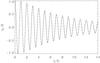 |
Fig. 1 Dependence of η on time found by the direct numerical modelling (solid line) and by solving Eq. (29) (dashed line) for ϵ = 0.1. |
Examination of Figs. 1–3 reveals that the solution can be written in the form η(t) = A(t)sin(ωt + Φ(t)). The phase shift Φ(t) is very small and we did not study it. Our attention was concentrated on the behaviour of the wave amplitude A(t), which is displayed in Figs. 4–6. In these figures the solid lines show ln (A/R) calculated using Eq. (29). The circles show the same quantity calculated using the direct numerical modelling. We see that for small t/Π the curves showing the dependence of ln (A/R) on time have a parabolic shape, while they are approximately linear for larger values of t/Π. The distance where the transition from the parabolic to linear shape occurs increases with the increase of ϵ. Hence the oscillation amplitude is described by a kind of Gaussian profile for small time and by the exponential function for larger time. This result is similar to one found by Pascoe et al. (2010, 2011, 2012) for propagating waves. The dashed line in Figs. 4–6 show ln(A/R) given by the classical theory of resonant absorption.
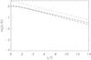 |
Fig. 4 Dependence of ln(A/R) on time for ϵ = 0.1. The solid line corresponds to the solution of Eq. (29). The circles show the result of the direct numerical modelling. The dashed line shows the linear dependence for large t. |
We calculate the damping time td defined by A(td)/R = e-1 and compare it with the damping time predicted by the classical theory of resonant absorption, tdc = 1/γd, where γd is given by Eq. (30). It follows both from the direct numerical modelling and from the solution of Eq. (29) that td/Π ≈ 8.8 for ϵ = 0.1, td/Π ≈ 4.6 for ϵ = 0.2, and td/Π ≈ 3.2 for ϵ = 0.3. Using Eq. (30) we obtain tdc/Π = 4(π2ϵκ)-1. As a result we find that td exceeds tdc by about 9% for ϵ = 0.1, about 14% for ϵ = 0.2, and about 18% for ϵ = 0.3. Hence, we conclude that the classical theory of resonant absorption underestimates the damping time and that the error grows when ϵ increases. However, the error is not very large, so the damping time given by the classical theory of resonant absorption can be taken as a reasonable approximation.
It is instructive to compare the results obtained in this paper with those obtained by Hood et al. (2013). These authors studied the resonant damping of propagating kink waves in a semi-infinite magnetic tube, where the waves are excited by a driver at the tube end. There is an obvious similarity between our results and those obtained by Hood et al. (2013). They found that the wave amplitude is approximately described by the Gaussian function at sufficiently small distance from the tube end, and we found that the oscillation amplitude is approximately described by the Gaussian function at sufficiently small time. Next, Hood et al. (2013) found that at larger distances the wave amplitude decays exponentially and that the distance where the transition from the Gaussian to the exponential amplitude profile occurs increases with the ϵ increase. We found that at larger time the oscillation amplitude decays exponentially and that the time when the transition from the Gaussian to the exponential amplitude profile occurs increases with the ϵ increase. Finally, Hood et al. (2013) found that the classical theory of resonant absorption underestimates the damping distance, while we found that it underestimates the damping time.
5. Summary and conclusions
In this paper we have studied the resonant damping of kink oscillations of a magnetic tube with the plasma density varying in the radial direction. The TTTB approximation and the approximation of cold plasmas were used. We derived the governing equation for the tube displacement (Eq. (29)).
To study the resonant damping of kink oscillations, we solved Eq. (29) numerically for various values of the ratio ϵ. This ratio compares the thickness of the inhomogeneous layer, where the plasma density varies, to the tube radius. We found that for sufficiently small time the amplitude decrease is described by a kind of Gaussian function, while it becomes exponential for larger time. The larger the ϵ, the later the transition from the Gaussian to the exponential regime occurs. The solutions to Eq. (29) were compared with the results of the direct numerical modelling, and the agreement was found to be fairly good.
We defined the damping time as the time when the oscillation amplitude decreases e times in comparison with its initial value. Then we calculated the damping time using Eq. (29) and compared it with that given by the classical theory of resonant absorption. We found that the classical theory underestimates the damping time, with the error getting larger when ϵ increases. However, this error is not very large. Even for ϵ = 0.3, which
is the largest value used in our study, the error is only about 18%. Hence, we conclude that the damping time given by the classical theory can be used as a reasonable approximation.
Online material
Appendix A: Asymptotic solution for large time
In this appendix we study the asymptotic behaviour of the solution to Eq. (29)
for ωt ~ ϵ-1. We introduce the Laplace
transform  = \int_0^t f(t) {\rm e}^{{\rm i}st} {\rm d}t . \label{eq:A1} \end{eqnarray}](/articles/aa/full_html/2013/07/aa20195-12/aa20195-12-eq131.png) (A.1)Applying
the Laplace transform to Eq. (29) and
using the theorem about the Laplace transform of convolution, we obtain
(A.1)Applying
the Laplace transform to Eq. (29) and
using the theorem about the Laplace transform of convolution, we obtain  = R\omega\frac{2 - \epsilon{\cal L}[F(t)](s/\omega)} {2(\omega^2 - s^2) - \epsilon\kappa\omega^2{\cal L}[G(t)](s/\omega)} \cdot \label{eq:A2} \end{eqnarray}](/articles/aa/full_html/2013/07/aa20195-12/aa20195-12-eq132.png) (A.2)Using
the standard table of Laplace transforms, we find
(A.2)Using
the standard table of Laplace transforms, we find  = \frac1{2s^2}\ln\frac{1 - s^2(1 - \kappa)} {1 - s^2(1 + \kappa)} \cdot \label{eq:A4} \end{eqnarray}](/articles/aa/full_html/2013/07/aa20195-12/aa20195-12-eq133.png) (A.3)We
do not give the expression
for ℒ [F(t)] (s) because it is
not used in what follows. The solution to Eq. (29) with the initial condition (17) is given by
(A.3)We
do not give the expression
for ℒ [F(t)] (s) because it is
not used in what follows. The solution to Eq. (29) with the initial condition (17) is given by \} {\rm e}^{-{\rm i}s\omega t}\,{\rm d}s} {2 - 2s^2 - \epsilon\kappa{\cal L}[G(t)](s)}, \label{eq:A5} \end{eqnarray}](/articles/aa/full_html/2013/07/aa20195-12/aa20195-12-eq135.png) (A.4)where ς
is any positive constant. When calculating the inverse Laplace transform, we have made
the substitution s = ωs′
and then dropped the prime.
(A.4)where ς
is any positive constant. When calculating the inverse Laplace transform, we have made
the substitution s = ωs′
and then dropped the prime.
Now we use Eq. (A.4) to obtain the
asymptotic expression for η(t) valid
for ωt ~ ϵ-1. The ratio of the second
term in the numerator of the integrand in Eq. (A.4) to the first one is of the order of ϵ. Hence, we can
neglect the second term in the numerator and use the approximate expression
} \label{eq:B1} \end{eqnarray}](/articles/aa/full_html/2013/07/aa20195-12/aa20195-12-eq139.png) (A.5)to
calculate the asymptotic behaviour of η(t) at large
time. The integrand in this expression has four logarithmic branch points
at s = ±s+ and
s = ±s−, where
(A.5)to
calculate the asymptotic behaviour of η(t) at large
time. The integrand in this expression has four logarithmic branch points
at s = ±s+ and
s = ±s−, where  (A.6)To
obtain a single-valued branch of the integrand, we make the cuts of the
complex s-plane along the
intervals [−s−, −s+]
and [s+, s−] .
The multivaluedness of the integrand is related to the presence of logarithm in
Eq. (A.3). We define the principal
sheet of the Riemann surface of the integrand by the condition that the imaginary part
of this logarithm is between −πi and πi. In what
follows we use the notation “ln” for this value of logarithm. All other values differ
from this value by 2πni, where n is an integer number.
(A.6)To
obtain a single-valued branch of the integrand, we make the cuts of the
complex s-plane along the
intervals [−s−, −s+]
and [s+, s−] .
The multivaluedness of the integrand is related to the presence of logarithm in
Eq. (A.3). We define the principal
sheet of the Riemann surface of the integrand by the condition that the imaginary part
of this logarithm is between −πi and πi. In what
follows we use the notation “ln” for this value of logarithm. All other values differ
from this value by 2πni, where n is an integer number.
The function  (A.7)maps
the complex s-plane with
cuts [−s−, −s+]
and [s+, s−]
on the
strip −π < ℑ(w) < π
in the complex w-plane, where ℑ indicates the imaginary part of a
quantity. We find the zeros of the denominator of the integrand in Eq. (A.5), which are determined by the equation
(A.7)maps
the complex s-plane with
cuts [−s−, −s+]
and [s+, s−]
on the
strip −π < ℑ(w) < π
in the complex w-plane, where ℑ indicates the imaginary part of a
quantity. We find the zeros of the denominator of the integrand in Eq. (A.5), which are determined by the equation
 (A.8)Let s∗
be a root of this equation. If it is not close to ±s±
then it follows that
(A.8)Let s∗
be a root of this equation. If it is not close to ±s±
then it follows that  . This implies that
either
. This implies that
either  or
or  .
In the first case we immediately see that the left-hand side of Eq. (A.8) is of the order
of ϵ2, so that the only possible solution of this kind
is s∗ = 0.
Since ℒ [G(t)] (0) = κ, it is
straightforward to see that the denominator of the integrand in Eq. (A.5) does not equal zero
when s = 0. Hence, s∗ = 0 is a spurious
root.
.
In the first case we immediately see that the left-hand side of Eq. (A.8) is of the order
of ϵ2, so that the only possible solution of this kind
is s∗ = 0.
Since ℒ [G(t)] (0) = κ, it is
straightforward to see that the denominator of the integrand in Eq. (A.5) does not equal zero
when s = 0. Hence, s∗ = 0 is a spurious
root.
Considering the second possibility, namely, ,
we look for the root to Eq. (A.8) in the
form s∗ = ±1 + ϵδ. By substituting
this expression in Eq. (A.8) we obtain
 (A.9)The
imaginary part of the left-hand side of this equation is close to −πi
when ℑ(±δ) < 0 and to πi
when ℑ(±δ) > 0. This implies that the
imaginary parts of the left- and right-hand side of Eq. (A.9) have different signs, so that this equation cannot have a
solution with ℑ(δ) ≠ 0. It also cannot have a real solution because in
that case the imaginary part of the right-hand side is zero, while the imaginary part of
the left-hand side is non-zero.
(A.9)The
imaginary part of the left-hand side of this equation is close to −πi
when ℑ(±δ) < 0 and to πi
when ℑ(±δ) > 0. This implies that the
imaginary parts of the left- and right-hand side of Eq. (A.9) have different signs, so that this equation cannot have a
solution with ℑ(δ) ≠ 0. It also cannot have a real solution because in
that case the imaginary part of the right-hand side is zero, while the imaginary part of
the left-hand side is non-zero.
Hence, Eq. (A.8) can only have
solutions close to ±s±. We look for the solution in the
form s∗ = ±s± + δ,
where δ ≪ 1. Substituting this expression in Eq. (A.8) we obtain four
roots,  and
and  ,
where
,
where ![Mathematical equation: \appendix \setcounter{section}{1} \begin{eqnarray} \bar{s}_\pm = \frac1{\sqrt{1\pm\kappa}}\left[1 \mp \frac\kappa{1\pm\kappa} \exp\left(-\frac4{\epsilon(1\pm\kappa)^2}\right)\right] \cdot \label{eq:B5} \end{eqnarray}](/articles/aa/full_html/2013/07/aa20195-12/aa20195-12-eq176.png) (A.10)Hence,
there are four poles on the real axis, at
and .
(A.10)Hence,
there are four poles on the real axis, at
and .
The integration contour in Eq. (A.5) is a straight line parallel to the real axis. Its equation in ℑ(s) = ς > 0. Since the integrand in Eq. (A.5) is an analytical function in the upper part of the complex s-plane, we can deform the integration contour arbitrarily without changing the value of the integral. The only conditions that have to be satisfied are that the new contour is completely in the union of the upper part of the complex s-plane and the real axis and that the part of the new contour that is on the real axis does not contain singularities of the integrand. It is convenient to use the new integration contour shown in Fig. A.1. This contour consists
 |
Fig. A.1 Integration contour used to obtain Eq. (A.11) is shown by the thick solid line. The dashed lines show the cuts. |
of five intervals of the real axis, ![Mathematical equation: \hbox{$(-\infty,-\bar{s}_- - \varepsilon]$}](/articles/aa/full_html/2013/07/aa20195-12/aa20195-12-eq178.png) ,
,
![Mathematical equation: \hbox{$[-\bar{s}_- + \varepsilon,-\bar{s}_+ - \varepsilon]$}](/articles/aa/full_html/2013/07/aa20195-12/aa20195-12-eq179.png) ,
,
![Mathematical equation: \hbox{$[-\bar{s}_+ + \varepsilon,\bar{s}_+ -\varepsilon]$}](/articles/aa/full_html/2013/07/aa20195-12/aa20195-12-eq180.png) ,
,
![Mathematical equation: \hbox{$[\bar{s}_+ + \varepsilon,\bar{s}_- -\varepsilon]$}](/articles/aa/full_html/2013/07/aa20195-12/aa20195-12-eq181.png) ,
and
,
and  ,
and four half-circles of radius ε centred
at
,
and four half-circles of radius ε centred
at  and
and  .
Taking ε → +0 we obtain
.
Taking ε → +0 we obtain }\nonumber\\ && - \frac{{\rm i}R}2\sum_{j=1}^4 \mbox{res}_{s=s_j}\frac{{\rm e}^{-{\rm i}s\omega t}}{2 - 2s^2 - \epsilon\kappa{\cal L}[G(t)](s)}, \end{eqnarray}](/articles/aa/full_html/2013/07/aa20195-12/aa20195-12-eq187.png) (A.11)where
(A.11)where  ,
,  ,
,  indicates the principal Cauchy part of an integral, and in the integrals along the
intervals [−s−, −s+]
and [s+, s−]
the integrand is calculated at the upper edges of the cuts.
indicates the principal Cauchy part of an integral, and in the integrals along the
intervals [−s−, −s+]
and [s+, s−]
the integrand is calculated at the upper edges of the cuts.
First of all, we note that } = A_j\exp(-C_j/\epsilon), \label{eq:B9} \end{eqnarray}](/articles/aa/full_html/2013/07/aa20195-12/aa20195-12-eq191.png) (A.12)where j = 1,2,3,4, Aj
and Cj are constants of the order of
unity, and Cj > 0.
This implies that the contribution of the last term in Eq. (A.11) is exponentially small and can be
neglected. Using the integration by parts we obtain
(A.12)where j = 1,2,3,4, Aj
and Cj are constants of the order of
unity, and Cj > 0.
This implies that the contribution of the last term in Eq. (A.11) is exponentially small and can be
neglected. Using the integration by parts we obtain } \nonumber=\\ && \frac {\rm i}{\omega t}\bigg[\frac{{\rm e}^{{\rm i}\omega ts_-}}{2 + 2s_-^2 - \epsilon\kappa{\cal L}[G(t)](s_-)} \\ && -\int_{-\infty}^{-s_-} {\rm e}^{-{\rm i}s\omega t} \frac {\rm d}{{\rm d}s}\left(\frac1{2 - 2s^2 - \epsilon\kappa{\cal L}[G(t)](s)}\right) {\rm d}s\bigg] .\nonumber \end{eqnarray}](/articles/aa/full_html/2013/07/aa20195-12/aa20195-12-eq196.png) (A.13)We
see that the contribution of the integral along the
interval (−∞, −s−] is of the order
of 1/ωt. Similarly we can show that the
contribution of the integrals along the
intervals [−s+, s+]
and [s−, ∞) are also of the order
of 1/ωt. Hence, we obtain
(A.13)We
see that the contribution of the integral along the
interval (−∞, −s−] is of the order
of 1/ωt. Similarly we can show that the
contribution of the integrals along the
intervals [−s+, s+]
and [s−, ∞) are also of the order
of 1/ωt. Hence, we obtain } \nonumber\\ && + {\cal O}(1/\omega t). \end{eqnarray}](/articles/aa/full_html/2013/07/aa20195-12/aa20195-12-eq201.png) (A.14)To
evaluate the asymptotic behaviour of the integrals in this expression, we need to make
the analytic continuation of the function w(s) on its
Riemann surface. This Riemann surface consists of an infinite set of complex planes with
cuts [−s−, −s+]
and [s+, s−]
properly attached to each other at the cuts. In what follows we use only two
non-principal sheets of the Riemann surface attached to the principal sheet at the upper
edges of the cuts. To define w(s) on the non-principal
sheet of the Riemann surface attached to the principal sheet at the upper edge of the
right cut, we consider a point s near this cut on the principal sheet.
We
write s = sr + isi,
where s+ < sr < s−
and |si| ≪ sr. Then
(A.14)To
evaluate the asymptotic behaviour of the integrals in this expression, we need to make
the analytic continuation of the function w(s) on its
Riemann surface. This Riemann surface consists of an infinite set of complex planes with
cuts [−s−, −s+]
and [s+, s−]
properly attached to each other at the cuts. In what follows we use only two
non-principal sheets of the Riemann surface attached to the principal sheet at the upper
edges of the cuts. To define w(s) on the non-principal
sheet of the Riemann surface attached to the principal sheet at the upper edge of the
right cut, we consider a point s near this cut on the principal sheet.
We
write s = sr + isi,
where s+ < sr < s−
and |si| ≪ sr. Then
 (A.15)and
we obtain
(A.15)and
we obtain  (A.16)We
assume that a point s on the principal Riemann sheet moves in such a
way that it crosses the right cut from the upper to the lower part of the complex plane,
i.e. ℑ(s) changes the sign from positive to negative. Then Eq. (A.16) implies that ℑ(w)
jumps by −2πi during this crossing. This means that to have the
continuous change of w(s) when s
moves from the upper part of the principal Riemann sheet to the lower part of the
non-principal Riemann sheet we have to define w(s) on
this non-principal sheet as
(A.16)We
assume that a point s on the principal Riemann sheet moves in such a
way that it crosses the right cut from the upper to the lower part of the complex plane,
i.e. ℑ(s) changes the sign from positive to negative. Then Eq. (A.16) implies that ℑ(w)
jumps by −2πi during this crossing. This means that to have the
continuous change of w(s) when s
moves from the upper part of the principal Riemann sheet to the lower part of the
non-principal Riemann sheet we have to define w(s) on
this non-principal sheet as  (A.17)In
a similar way we find that the analytic continuation
of w(s) on the non-principal Riemann sheet attached
to the principal sheet at the upper edge at the left cut is defined by
(A.17)In
a similar way we find that the analytic continuation
of w(s) on the non-principal Riemann sheet attached
to the principal sheet at the upper edge at the left cut is defined by  (A.18)To
calculate the integral along the
interval [s+, s−]
in Eq. (A.14), we use the contour shown
in Fig. A.2. It consists of the
interval [s+, s−]
at the upper edge of the right cut on the principal Riemann sheet, two vertical lines
from s+
to s+ − ib and
from s−
to s− − ib on the non-principal Riemann
sheet, and the horizontal line connecting the
points s+ − ib
and s− − ib, once again on the
non-principal Riemann sheet. Here b > 0. To
calculate the integral along this contour we need to find the poles of the integrand
inside this contour. These poles coincide with the zeros
(A.18)To
calculate the integral along the
interval [s+, s−]
in Eq. (A.14), we use the contour shown
in Fig. A.2. It consists of the
interval [s+, s−]
at the upper edge of the right cut on the principal Riemann sheet, two vertical lines
from s+
to s+ − ib and
from s−
to s− − ib on the non-principal Riemann
sheet, and the horizontal line connecting the
points s+ − ib
and s− − ib, once again on the
non-principal Riemann sheet. Here b > 0. To
calculate the integral along this contour we need to find the poles of the integrand
inside this contour. These poles coincide with the zeros
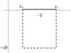 |
Fig. A.2 Integration contour used to calculate the integral along the interval [s+, s−] in Eq. (A.14). The solid line indicates the part of the contour that coincides with the upper edge of the right cut on the principal Riemann sheet. The dashed-dotted line indicates the parts of the contour on the non-principal Riemann sheet. The dashed line shows the cut. |
of Eq. (A.8). Since the area enclosed by the contour is on the non-principal Riemann sheet, we look for zeros of Eq. (A.8) on this sheet.
Although w(s) is now not given by Eq. (A.7) but by Eq. (A.17), the roots of Eq. (A.8) are still close to either 0 or 1 or to
one of the numbers ±s±. Obviously, the root close to 0
cannot be inside the contour. Simple analysis shows that there are roots close
to ±s− and ±s+, but
their real parts are equal to
and ,
respectively, so these roots are also not inside the contour. Finally, the root close
to 1 is given by  (A.19)This
root is inside the contour. Hence,
(A.19)This
root is inside the contour. Hence,
}=\nonumber\\ && -2\pi {\rm i} \mbox{res}_{s=\bar{s}} \frac{{\rm e}^{-{\rm i}s\omega t}\,{\rm d}s} {2 - 2s^2 - \epsilon\kappa{\cal L}[G(t)](s)} \cdot \end{eqnarray}](/articles/aa/full_html/2013/07/aa20195-12/aa20195-12-eq223.png) (A.20)We
estimate the integrals along the parts of the closed contour that are on the
non-principal Riemann sheet. Using the integration by parts we have
(A.20)We
estimate the integrals along the parts of the closed contour that are on the
non-principal Riemann sheet. Using the integration by parts we have }= \nonumber\\ && \int_0^b \frac{\exp[-\omega t(\sigma + {\rm i}s_-)]\,{\rm d}s}{2{\rm i} - 2{\rm i}(s_- - {\rm i} \sigma)^2 - {\rm i} \epsilon\kappa{\cal L}[G(t)](s_- - {\rm i}\sigma)} \to \frac{{\rm e}^{-{\rm i} \omega t s_-}}{\omega t} \int_0^\infty {\rm e}^{-\omega t\sigma} \nonumber\\ &&\times \frac {\rm d}{{\rm d}\sigma}\left(\frac1{2{\rm i} - 2{\rm i} (s_- - {\rm i}\sigma)^2 - {\rm i} \epsilon\kappa{\cal L}[G(t)](s_- - {\rm i}\sigma)}\right){\rm d} \sigma, \end{eqnarray}](/articles/aa/full_html/2013/07/aa20195-12/aa20195-12-eq224.png) (A.21)where
the limit is taken as b → ∞. In the same way we prove that the integral
along the vertical line connecting the
points s+ − ib
and s+ is of the order
of 1/ωt. Finally, the integral along the
horizontal line connecting the
points s− − ib
and s+ − ib tends to zero
as b → ∞. As a result we have
(A.21)where
the limit is taken as b → ∞. In the same way we prove that the integral
along the vertical line connecting the
points s+ − ib
and s+ is of the order
of 1/ωt. Finally, the integral along the
horizontal line connecting the
points s− − ib
and s+ − ib tends to zero
as b → ∞. As a result we have } \!=\! \widetilde{C} {\rm e}^{-{\rm i}\omega t} \exp\bigg(-\frac{\pi\epsilon\kappa\omega t}8\bigg) + {\cal O}(1/\omega t), \label{eq:B19} \end{eqnarray}](/articles/aa/full_html/2013/07/aa20195-12/aa20195-12-eq226.png) (A.22)}where
(A.22)}where
 is a
complex constant. In a similar way we can obtain a similar expression for the integral
along the
interval [−s−, −s+] .
is a
complex constant. In a similar way we can obtain a similar expression for the integral
along the
interval [−s−, −s+] .
It is worth explaining why we cannot prove in the same way that the integral along the interval [s+, s−] is of the order of 1/ωt.
The reason is that there is a pole at  ,
which is close to the
interval [s+, s−] .
After the integration by parts we obtain 1/ωt times
an integral. The integrand in this integral is very big, in the vicinity
of s = 1, so the whole product is not of the order
of 1/ωt.
,
which is close to the
interval [s+, s−] .
After the integration by parts we obtain 1/ωt times
an integral. The integrand in this integral is very big, in the vicinity
of s = 1, so the whole product is not of the order
of 1/ωt.
Summarising the analysis of this section, we arrive at the asymptotic expression
 (A.23)where C
is a complex constant and c.c. denotes complex conjugate.
(A.23)where C
is a complex constant and c.c. denotes complex conjugate.
Acknowledgments
M.S.R. acknowledges the support by a Royal Society Leverhulme Trust Senior Research Fellowship and by an STFC grant. J.T. acknowledges support from the Spanish Ministerio de Educación y Ciencia through a Ramón y Cajal grant and financial support from MICINN/MINECO and FEDER Funds through grant AYA2011-22846 Funding from CAIB through the “Grups Competitius” scheme and FEDER Funds is also acknowledged.
References
- Aschwanden, M. J., Fletcher, L., Schrijver, C. J., & Alexander, D. 1999, ApJ, 520, 880 [NASA ADS] [CrossRef] [Google Scholar]
- Goossens, M., Hollweg, J. V., & Sakurai, T. 1992, Sol. Phys., 138, 233 [NASA ADS] [CrossRef] [Google Scholar]
- Goossens, M., Ruderman, M. S., & Hollweg, J. V. 1995, Sol. Phys., 157, 75 [NASA ADS] [CrossRef] [Google Scholar]
- Goossens, M., Andries, J., & Aschwanden, M. J. 2002, A&A, 394, L39 [NASA ADS] [CrossRef] [EDP Sciences] [Google Scholar]
- Goossens, M., Erdélyi, R., & Ruderman, M. S. 2011, Space Sci. Rev., 158, 289 [NASA ADS] [CrossRef] [Google Scholar]
- Hollweg, J. V., & Yang, G. 1988, J. Geophys. Res., 93, 5423 [NASA ADS] [CrossRef] [Google Scholar]
- Hood, A. W., Ruderman, M. S., De Moortel, I., et al. 2013, A&A, 551, A39 [NASA ADS] [CrossRef] [EDP Sciences] [Google Scholar]
- Kappraff, J. M., & Tataronis, J. A. 1977, J. Plasma Phys., 18, 209 [NASA ADS] [CrossRef] [Google Scholar]
- Mann, I. R., Wright, A. N., & Cally, P. S. 1995, J. Geophys. Res., 100, 19441 [NASA ADS] [CrossRef] [Google Scholar]
- Mok, Y., & Einaudi, G. 1985, J. Plasma Phys., 33, 199 [NASA ADS] [CrossRef] [Google Scholar]
- Nakariakov, V. M., Ofman, L., Deluca, E. E., Roberts, B., & Davila, J. M. 1999, Science, 285, 862 [NASA ADS] [CrossRef] [PubMed] [Google Scholar]
- Pascoe, D. J., Wright, A. N., & De Moortel, I. 2010, ApJ, 711, 990 [NASA ADS] [CrossRef] [Google Scholar]
- Pascoe, D. J., Wright, A. N., & De Moortel, I. 2011, ApJ, 731, 73 [NASA ADS] [CrossRef] [Google Scholar]
- Pascoe, D. J., Hood, A. W., De Mortel, I., & Wright, A. N. 2012, ApJ, 539, A37 [Google Scholar]
- Ofman, L., & Aschwanden, M. J. 2002, ApJ, 576, L153 [NASA ADS] [CrossRef] [Google Scholar]
- Poedts, S., Goossens, M., & Kerner, W. 1990, Comput. Phys. Commun., 59, 95 [NASA ADS] [CrossRef] [Google Scholar]
- Priest, E. 1982, Solar Magneto-Hydrodynamics, Geophysics and Astrophysics Monographs (Kluwer Academic Publishers) [Google Scholar]
- Ruderman, M. S. 2011, A&A, 534, A78 [NASA ADS] [CrossRef] [EDP Sciences] [Google Scholar]
- Ruderman, M. S., & Roberts, B. 2002, ApJ, 577, 475 [NASA ADS] [CrossRef] [Google Scholar]
- Ruderman, M. S., Tirry, W., & Goossens, M. 1995, J. Plasma Phys., 54, 129 [NASA ADS] [CrossRef] [Google Scholar]
- Ruderman, M. S., Goossens, M., & Andries, J. 2010, Phys. Plasmas, 17, 082108 [NASA ADS] [CrossRef] [Google Scholar]
- Sakurai, T., Goossens, M., & Hollweg, J. V. 1991, Sol. Phys., 133, 227 [NASA ADS] [CrossRef] [Google Scholar]
- Sedláček, Z. 1971, J. Plasma Phys., 5, 239 [NASA ADS] [CrossRef] [Google Scholar]
- Soler, R., Terradas, J., & Goossens, M. 2011, ApJ, 734, 80 [NASA ADS] [CrossRef] [Google Scholar]
- Terradas, J., Oliver, R., & Ballester, J. L. 2006, ApJ, 642, 533 [NASA ADS] [CrossRef] [Google Scholar]
- Terradas, J., Goossens, M., & Verth, G. 2010, A&A, 524, A23 [NASA ADS] [CrossRef] [EDP Sciences] [Google Scholar]
- Tirry, W. J., & Goossens, M. 1996, ApJ, 471, 501 [NASA ADS] [CrossRef] [Google Scholar]
All Figures
|
Fig. 1 Dependence of η on time found by the direct numerical modelling (solid line) and by solving Eq. (29) (dashed line) for ϵ = 0.1. |
| In the text | |
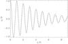 |
Fig. 2 Same as Fig. 1, but for ϵ = 0.2. |
| In the text | |
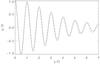 |
Fig. 3 Same as Fig. 1, but for ϵ = 0.3. |
| In the text | |
|
Fig. 4 Dependence of ln(A/R) on time for ϵ = 0.1. The solid line corresponds to the solution of Eq. (29). The circles show the result of the direct numerical modelling. The dashed line shows the linear dependence for large t. |
| In the text | |
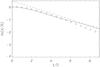 |
Fig. 5 Same as Fig. 4, but for ϵ = 0.2. |
| In the text | |
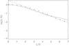 |
Fig. 6 Same as Fig. 4, but for ϵ = 0.3. |
| In the text | |
|
Fig. A.1 Integration contour used to obtain Eq. (A.11) is shown by the thick solid line. The dashed lines show the cuts. |
| In the text | |
|
Fig. A.2 Integration contour used to calculate the integral along the interval [s+, s−] in Eq. (A.14). The solid line indicates the part of the contour that coincides with the upper edge of the right cut on the principal Riemann sheet. The dashed-dotted line indicates the parts of the contour on the non-principal Riemann sheet. The dashed line shows the cut. |
| In the text | |
Current usage metrics show cumulative count of Article Views (full-text article views including HTML views, PDF and ePub downloads, according to the available data) and Abstracts Views on Vision4Press platform.
Data correspond to usage on the plateform after 2015. The current usage metrics is available 48-96 hours after online publication and is updated daily on week days.
Initial download of the metrics may take a while.