© ESO, 2012

1. Introduction

Huge cosmological surveys are currently ongoing or planned for the near future. The large statistical power of these surveys allows us to study the statistical properties of the cosmological fields well beyond the lowest, second-order statistical level. In order to employ these higher-order statistics in obtaining information about the underlying cosmology, one needs to be able to accurately predict these statistics as a function of the model parameters. Moreover, one also needs to predict the expected errors on these higher-order measures, i.e., the covariance of higher-order statistics.

Whereas there exist rather accurate fitting formulae for the power spectrum of the cosmic density field (e.g., Peacock & Dodds 1996; Smith et al. 2003), this is no longer the case for higher-order statistical properties. For example, the semi-empirical fitting formula for the bispectrum of the cosmic density field (Scoccimarro & Couchman 2001) is estimated to be accurate only at the level of several tens of percent.

In order to obtain the covariance of the power spectrum and the bispectrum, even higher-order statistical properties of the field need to be known. The power spectrum covariance depends on fourth-order statistical properties, i.e., the trispectrum, which is even harder to predict. In principle, one needs to understand the sixth-order properties of the field in order to determine the covariance of the bispectrum.

However, depending on the statistical field under consideration, certain simplifications may apply. In particular, if the density field is sufficiently close to a Gaussian field, the higher-order terms in the covariance of the power spectrum and the bispectrum may become subdominant, in which case they can be obtained solely from the power spectrum itself.

In this paper we study the covariance of the bispectrum for two-dimensional random fields. Whereas our prime interest is focused on the convergence field of cosmic shear (as a prime example of a two-dimensional cosmological field) (for a review of gravitational lensing, see Schneider 2006), our results are not restricted to this particular application.

Third-order cosmic shear statistics is known to provide very valuable information, complementary to that from the cosmic shear power spectrum (e.g., Takada & Jain 2004; Kilbinger & Schneider 2005; Huterer et al. 2006), which is confirmed by the first measurements of third-order cosmic shear in previous surveys (Bernardeau et al. 2002; Pen et al. 2003; Jarvis et al. 2004; Semboloni et al. 2011). Ongoing and future surveys, such as the Canada-France-Hawaii-Telescope Legacy Survey (CFHTLS), the KIlo-Degree Survey (KIDS), the Dark Energy Survey (DES) and EUCLID, will measure the third-order cosmic shear signal with very high accuracy. However, estimating the statistical power of these surveys, and obtaining realistic confidence estimates for model parameters, remains a challenge that hinges on our ability to estimate the bispectrum covariance.

Hu (2000) estimated this covariance by analogy to the bispectrum covariance of the cosmic microwave background. As discussed in Joachimi et al. (2009, hereafter JSS), this approach has a number of drawbacks that result from the use of spherical harmonics in the analysis. Instead, JSS derived a general expression for the bispectrum covariance on a finite region in the flat-sky limit, which can be separated into four terms. The first term contains the contribution of the power spectrum to the bispectrum covariance, and is the only term relevant for Gaussian random fields. The other three terms contain the contributions of the bispectrum, the trispectrum and the pentaspectrum. Dropping these higher-order terms in the expression is usually termed the Gaussian approximation of the bispectrum covariance. If the other terms were small for realistic cosmic fields, this would tremendously simplify the estimation of confidence regions from third-order statistics. At first glance this seems to be invalid as the present density field appears to be highly non-Gaussian, especially on small scales. Nevertheless, this Gaussian approximation has been employed in nearly all studies of parameter forecasts from third-order cosmic shear (e.g., Takada & Jain 2004; Huterer et al. 2006; Shi et al. 2010).

In this paper, we investigate the validity of the Gaussian approximation, using simulated random fields with different degrees of non-Gaussianity. Specifically, we employ log-normal random fields which we characterise by the non-Gaussianity parameter α. As argued in the seminal paper by Coles & Jones (1991), matter density fields are well described by log-normal statistics, making these statistics relevant in a cosmological context. Indeed, as Kayo et al. (2001) have shown, the distribution of the density fluctuations in the universe can rather well be described by a log-normal distribution. Moreover, Taruya et al. (2002) and Hilbert et al. (2011) have shown that the same holds true for the cosmic shear convergence field, which serves as justification for using these particular non-Gaussian fields for our study. Furthermore, Hilbert et al. (2011) employed the log-normal ansatz to calculate the covariance of the power spectrum of cosmic shear fields; they showed that this model provides fairly accurate results, when compared to ray-tracing simulations. However, we caution that the log-normal approach has yet not been shown to give a realistic approximation for higher-order correlation functions and that the log-normal is not completely determined by its moments (Coles & Jones 1991; Carron & Neyrinck 2012). To circumvent the assumption of a probability distribution for todays cosmic fields, one would need N-body simulations, which are – given the high number of realisations required for our purpose – currently not available to us. Moreover, the log-normal approach allows us to tune the degree of non-Gaussianity α very easily, which is a necessity to answer the question: to which degree of non-Gaussianity is it justified to use the Gaussian approximation for the bispectrum covariance?

This paper is organised as follows: Sect. 2 reviews the most important properties of the analytical formula for the bispectrum covariance derived by JSS and the corresponding Gaussian approximation, as well as an ansatz to determine the scope of validity of the latter applied to non-Gaussian fields. In Sect. 3 the primary quantities in the theoretical framework of log-normal random fields are introduced, and the method we used to numerically generate the random fields. The results will be presented, analysed and discussed in Sect. 4. Finally, Sect. 5 provides conclusions.

2. The bispectrum covariance: analytical formula and Gaussian approximation

In general, the bispectrum of a two-dimensional homogeneous and isotropic random field in Fourier space f(ℓ) with zero mean is defined by $⟨\mathit{f}\mathrm{\left(}{\ell }\mathrm{1}\mathrm{\right)}\mathit{f}\mathrm{\left(}{\ell }\mathrm{2}\mathrm{\right)}\mathit{f}\mathrm{\left(}{\ell }\mathrm{3}\mathrm{\right)}⟩\mathrm{=}\mathrm{\left(}\mathrm{2}\mathit{\pi }{\mathrm{)}}^{\mathrm{2}}{\mathit{\delta }}_{\mathrm{D}}^{\mathrm{\left(}\mathrm{2}\mathrm{\right)}}\mathrm{\right(}{\ell }\mathrm{1}\mathrm{+}{\ell }\mathrm{2}\mathrm{+}{\ell }\mathrm{3}\mathrm{\left)}\mathit{B}\mathrm{\right(}{\mathit{\ell }}_{\mathrm{1}}\mathit{,}{\mathit{\ell }}_{\mathrm{2}}\mathit{,}{\mathit{\ell }}_{\mathrm{3}}\mathrm{)}\mathit{,}$(1)and consequently depends on the length ℓ_i = |ℓ_i| of the three angular frequency vectors ℓ₁,ℓ₂,ℓ₃. It is characterised by the fact that the two-dimensional Dirac delta-distribution ${\mathit{\delta }}_{\mathrm{D}}^{\mathrm{\left(}\mathrm{2}\mathrm{\right)}}\mathrm{\left(}{\ell }\mathrm{\right)}$ restricts the three angular frequency vectors to form a triangle. Accordingly, JSS introduced the following bispectrum estimator for a random field of size Ω, $\begin{array}{ccc}\mathit{B̂}\mathrm{\left(}\mathit{\ell ̅}\mathrm{1}\mathit{,}\mathit{\ell ̅}\mathrm{2}\mathit{,}\mathit{\ell ̅}\mathrm{3}\mathrm{\right)}& \mathrm{:}\mathrm{=}& \frac{\mathrm{(}\mathrm{2}\mathit{\pi }{\mathrm{)}}^{\mathrm{2}}}{\mathrm{\Omega }}{\mathrm{\Lambda }}^{-1}\mathrm{(}\mathit{\ell ̅}\mathrm{1}\mathit{,}\mathit{\ell ̅}\mathrm{2}\mathit{,}\mathit{\ell ̅}{\mathrm{3}}^{\mathrm{)}}\\ & & \end{array}$(2)so that the bispectrum can be calculated by averaging configurations over annuli. The mean length of a triangle side, corresponding to the mean radius of an annulus, is denoted by $\overline{{\mathit{\ell }}_{\mathit{i}}}$ and the corresponding area of an annulus is given by ${\mathit{A}}_{\mathit{R}}\mathrm{\left(}\overline{{\mathit{\ell }}_{\mathit{i}}}\mathrm{\right)}\mathrm{=}\mathrm{2}\mathit{\pi }\overline{{\mathit{\ell }}_{\mathit{i}}}\mathrm{\Delta }{\mathit{\ell }}_{\mathit{i}}$, with Δℓ_i being the respective bin size. The parameter ${\mathrm{\Lambda }}^{-1}\mathrm{\left(}\overline{{\mathit{\ell }}_{\mathrm{1}}}\mathit{,}\overline{{\mathit{\ell }}_{\mathrm{2}}}\mathit{,}\overline{{\mathit{\ell }}_{\mathrm{3}}}\mathrm{\right)}\mathrm{=}\frac{\mathrm{1}}{\mathrm{4}}\sqrt{\mathrm{2}\mathit{\ell ̅}\begin{array}{}\mathrm{2}\\ \mathrm{1}\end{array}\mathit{\ell ̅}\begin{array}{}\mathrm{2}\\ \mathrm{2}\end{array}\mathrm{+}\mathrm{2}\mathit{\ell ̅}\begin{array}{}\mathrm{2}\\ \mathrm{1}\end{array}\mathit{\ell ̅}\begin{array}{}\mathrm{2}\\ \mathrm{3}\end{array}\mathrm{+}\mathrm{2}\mathit{\ell ̅}\begin{array}{}\mathrm{2}\\ \mathrm{2}\end{array}\mathit{\ell ̅}\begin{array}{}\mathrm{2}\\ \mathrm{3}\end{array}\mathrm{-}\mathit{\ell ̅}\begin{array}{}\mathrm{4}\\ \mathrm{1}\end{array}\mathrm{-}\mathit{\ell ̅}\begin{array}{}\mathrm{4}\\ \mathrm{2}\end{array}\mathrm{-}\mathit{\ell ̅}\begin{array}{}\mathrm{4}\\ \mathrm{3}\end{array}}\hspace{0.17em}$(3)reflects the area of the triangle which is spanned by the three wave vectors. JSS showed that the estimator (2) is unbiased in the limit of small annuli width Δℓ_i.

JSS derived an analytical expression for the covariance of the bispectrum estimator defined in Eq. (2), $\begin{array}{ccc}\mathrm{Cov}\left(\mathit{B̂}\mathrm{\left(}\mathit{\ell ̅}\mathrm{1}\mathit{,}\mathit{\ell ̅}\mathrm{2}\mathit{,}\mathit{\ell ̅}\mathrm{3}\mathrm{\right)}\mathit{,}\hspace{0.17em}\mathit{B̂}\mathrm{\left(}\mathit{\ell ̅}\mathrm{4}\mathit{,}\mathit{\ell ̅}\mathrm{5}\mathit{,}\mathit{\ell ̅}\mathrm{6}\mathrm{\right)}\right)& \mathrm{=}& \mathit{\gamma P}\mathrm{\left(}\mathit{\ell ̅}\mathrm{1}\mathrm{\right)}\mathit{P}\mathrm{\left(}\mathit{\ell ̅}\mathrm{2}\mathrm{\right)}\mathit{P}\mathrm{\left(}\mathit{\ell ̅}\mathrm{3}\mathrm{\right)}\\ & \mathrm{+}& \end{array}$(4)This expression consists of four different terms. The first term is proportional to the third power of the power spectrum, with an amplitude given by the geometrical factor $\mathit{\gamma }\mathrm{:}\mathrm{=}\frac{\mathrm{(}\mathrm{2}\mathit{\pi }{\mathrm{)}}^{\mathrm{3}}}{\mathrm{\Omega }\mathit{\ell ̅}\mathrm{1}\mathit{\ell ̅}\mathrm{2}\mathit{\ell ̅}\mathrm{3}\mathrm{\Delta }{\mathit{\ell }}_{\mathrm{1}}\mathrm{\Delta }{\mathit{\ell }}_{\mathrm{2}}\mathrm{\Delta }{\mathit{\ell }}_{\mathrm{3}}}{\mathrm{\Lambda }}^{-1}\mathrm{(}\mathit{\ell ̅}\mathrm{1}\mathit{,}\mathit{\ell ̅}\mathrm{2}\mathit{,}\mathit{\ell ̅}{\mathrm{3}}^{\mathrm{)}}{\mathit{D}}_{\mathit{\ell ̅}\mathrm{1}\mathit{,}\mathit{\ell ̅}\mathrm{2}\mathit{,}\mathit{\ell ̅}\mathrm{3}\mathit{,}\mathit{\ell ̅}\mathrm{4}\mathit{,}\mathit{\ell ̅}\mathrm{5}\mathit{,}\mathit{\ell ̅}\mathrm{6}}\mathit{,}$(5)with the short hand notation $\begin{array}{ccc}{\mathit{D}}_{\mathit{\ell ̅}\mathrm{1}\mathit{,}\mathit{\ell ̅}\mathrm{2}\mathit{,}\mathit{\ell ̅}\mathrm{3}\mathit{,}\mathit{\ell ̅}\mathrm{4}\mathit{,}\mathit{\ell ̅}\mathrm{5}\mathit{,}\mathit{\ell ̅}\mathrm{6}}& \mathrm{=}& {\mathit{\delta }}_{\mathit{\ell ̅}\mathrm{1}\mathit{\ell ̅}\mathrm{4}}{\mathit{\delta }}_{\mathit{\ell ̅}\mathrm{2}\mathit{\ell ̅}\mathrm{5}}{\mathit{\delta }}_{\mathit{\ell ̅}\mathrm{3}\mathit{\ell ̅}\mathrm{6}}\mathrm{+}{\mathit{\delta }}_{\mathit{\ell ̅}\mathrm{1}\mathit{\ell ̅}\mathrm{5}}{\mathit{\delta }}_{\mathit{\ell ̅}\mathrm{2}\mathit{\ell ̅}\mathrm{4}}{\mathit{\delta }}_{\mathit{\ell ̅}\mathrm{3}\mathit{\ell ̅}\mathrm{6}}\\ & \mathrm{+}& {\mathit{\delta }}_{\mathit{\ell ̅}\mathrm{1}\mathit{\ell ̅}\mathrm{4}}{\mathit{\delta }}_{\mathit{\ell ̅}\mathrm{2}\mathit{\ell ̅}\mathrm{6}}{\mathit{\delta }}_{{\mathit{\ell }}_{\mathrm{3}}{\mathit{\ell }}_{\mathrm{5}}}\mathrm{+}{\mathit{\delta }}_{\mathit{\ell ̅}\mathrm{1}\mathit{\ell ̅}\mathrm{5}}{\mathit{\delta }}_{\mathit{\ell ̅}\mathrm{2}\mathit{\ell ̅}\mathrm{6}}{\mathit{\delta }}_{\mathit{\ell ̅}\mathrm{3}\mathit{\ell ̅}\mathrm{4}}\\ & \mathrm{+}& {\mathit{\delta }}_{\mathit{\ell ̅}\mathrm{1}\mathit{\ell ̅}\mathrm{6}}{\mathit{\delta }}_{\mathit{\ell ̅}\mathrm{2}\mathit{\ell ̅}\mathrm{4}}{\mathit{\delta }}_{\mathit{\ell ̅}\mathrm{3}\mathit{\ell ̅}\mathrm{5}}\mathrm{+}{\mathit{\delta }}_{\mathit{\ell ̅}\mathrm{1}\mathit{\ell ̅}\mathrm{6}}{\mathit{\delta }}_{\mathit{\ell ̅}\mathrm{2}\mathit{\ell ̅}\mathrm{5}}{\mathit{\delta }}_{\mathit{\ell ̅}\mathrm{3}\mathit{\ell ̅}\mathrm{4}}\mathit{,}\end{array}$(6)and δ_xy = 1 if x = y, and zero otherwise. In the case of a Gaussian field, this would be the sole contribution to the covariance; therefore, the approximation of the bispectrum covariance by this first term only is called Gaussian approximation in the following. The other three terms account for the contribution of higher-order spectra to the bispectrum covariance: the second term is an integral over the product of bispectra, the third term an integral over the product of the trispectrum and the power spectrum, and finally the fourth term an integral over the pentaspectrum.

Due to the complexity of Eq. (4) and the fact that higher-order spectra are usually much more difficult to obtain, either analytically or from simulations, usually only the Gaussian approximation is used for statistical analyses of cosmological fields, despite the fact that these fields are not purely Gaussian (see Sect. 1). Thus the question arises to which degree of non-Gaussianity of the underlying field it is justified to use the Gaussian approximation for computing the bispectrum covariance. We have addressed the problem by the following approach: applied to a purely Gaussian random field, the Gaussian approximation should hold per definition, ${\mathrm{Cov}}_{\mathrm{G}}\left(\mathit{B̂}\mathrm{\left(}\mathit{\ell ̅}\mathrm{1}\mathit{,}\mathit{\ell ̅}\mathrm{2}\mathit{,}\mathit{\ell ̅}\mathrm{3}\mathrm{\right)}\mathit{,}\hspace{0.17em}\mathit{B̂}\mathrm{\left(}\mathit{\ell ̅}\mathrm{4}\mathit{,}\mathit{\ell ̅}\mathrm{5}\mathit{,}\mathit{\ell ̅}\mathrm{6}\mathrm{\right)}\right)\mathrm{=}\mathit{\gamma }{\mathit{P}}_{\mathrm{G}}\mathrm{\left(}\mathit{\ell ̅}\mathrm{1}\mathrm{\right)}{\mathit{P}}_{\mathrm{G}}\mathrm{\left(}\mathit{\ell ̅}\mathrm{2}\mathrm{\right)}{\mathit{P}}_{\mathrm{G}}\mathrm{\left(}\mathit{\ell ̅}\mathrm{3}\mathrm{\right)}\mathit{,}$(7)as will nevertheless be investigated numerically in Sect. 4.3.1. However, for a non-Gaussian random field, the Gaussian approximation might hold to a certain degree of non-Gaussianity α (which will be specified in Sect. 3.1) as well, ${\mathrm{Cov}}_{\mathit{\alpha }}\left(\mathit{B̂}\mathrm{\left(}\mathit{\ell ̅}\mathrm{1}\mathit{,}\mathit{\ell ̅}\mathrm{2}\mathit{,}\mathit{\ell ̅}\mathrm{3}\mathrm{\right)}\mathit{,}\hspace{0.17em}\mathit{B̂}\mathrm{\left(}\mathit{\ell ̅}\mathrm{4}\mathit{,}\mathit{\ell ̅}\mathrm{5}\mathit{,}\mathit{\ell ̅}\mathrm{6}\mathrm{\right)}\right)\mathrm{\approx }\mathit{\gamma }{\mathit{P}}_{\mathit{\alpha }}\mathrm{\left(}\mathit{\ell ̅}\mathrm{1}\mathrm{\right)}{\mathit{P}}_{\mathit{\alpha }}\mathrm{\left(}\mathit{\ell ̅}\mathrm{2}\mathrm{\right)}{\mathit{P}}_{\mathit{\alpha }}\mathrm{\left(}\mathit{\ell ̅}\mathrm{3}\mathrm{\right)}\mathit{.}$(8)In order to assess the range of validity of the Gaussian approximation for non-Gaussian random fields, we can compare a Gaussian random field with a non-Gaussian one, characterised by the degree of non-Gaussianity α, both having the same field geometry to assure the same geometrical factor γ for both fields. The quality of the Gaussian approximation can then be quantified, on the one hand, by a parameter ς, which is defined by $\begin{array}{ccc}\mathit{\varsigma }\mathrm{\left(}\mathit{\alpha }\mathrm{\right)}& \mathrm{=}& \frac{{\mathrm{Cov}}_{\mathit{\alpha }}\left(\mathit{B̂}\mathrm{\left(}\mathit{\ell ̅}\mathrm{1}\mathit{,}\mathit{\ell ̅}\mathrm{2}\mathit{,}\mathit{\ell ̅}\mathrm{3}\mathrm{\right)}\mathit{,}\hspace{0.17em}\mathit{B̂}\mathrm{\left(}\mathit{\ell ̅}\mathrm{1}\mathit{,}\mathit{\ell ̅}\mathrm{2}\mathit{,}\mathit{\ell ̅}\mathrm{3}\mathrm{\right)}\right)}{{\mathit{P}}_{\mathit{\alpha }}\mathrm{\left(}\mathit{\ell ̅}\mathrm{1}\mathrm{\right)}{\mathit{P}}_{\mathit{\alpha }}\mathrm{\left(}\mathit{\ell ̅}\mathrm{2}\mathrm{\right)}{\mathit{P}}_{\mathit{\alpha }}\mathrm{\left(}\mathit{\ell ̅}\mathrm{3}\mathrm{\right)}}\\ & \mathrm{\times }& \end{array}$(9)The first term on the right side corresponds to the geometrical factor γ defined in Eq. (8), the second term to γ^-1 defined in Eq. (7). As long as these two factors give the same result, ς(α) ≈ 1 and the Gaussian approximation provides a reasonable description of the diagonal part of the bispectrum covariance. On the other hand, one needs to check whether the true covariance matrix is (close to) diagonal, as predicted in the Gaussian approximation.

3. Methods

3.1. Log-normal random fields

To estimate the parameter ς(α), we consider a particular case of a non-Gaussian field, namely a log-normal field. This is motivated by its relative simplicity, as well as the fact that the density fluctuations in cosmological models can reasonably well be approximated by a log-normal distribution (see Sect. 1). The transformation of a two-dimensional homogeneous and isotropic Gaussian random field g(x) with zero mean and unit variance to a homogeneous and isotropic two-dimensional log-normal random field L(x) is given by $\mathit{L}\mathrm{\left(}{x}\mathrm{\right)}\mathrm{=}\frac{\mathit{A}}{\mathit{c}}\hspace{0.17em}\mathrm{(}{\mathrm{e}}^{\mathit{\alpha }\hspace{0.17em}\mathit{g}\mathrm{\left(}{x}\mathrm{\right)}}\mathrm{-}{\mathit{c}}^{\mathrm{)}}\mathit{.}$(10)The parameter α controls the deviation of the log-normal field from the initial Gaussian field and thus the degree of non-Gaussianity of the former. The parameter c and A are chosen as such that the log-normal field has zero mean and unit variance, $\begin{array}{ccc}{\mathit{\mu }}_{\mathit{\alpha }}& \mathrm{=}& ⟨\mathit{L}\mathrm{\left(}{x}\mathrm{\right)}⟩\mathrm{=}{\mathrm{\int }}_{\mathrm{-}\mathrm{\infty }}^{\mathrm{\infty }}\mathrm{d}\mathit{g}\mathrm{\left(}{x}\mathrm{\right)} \mathit{L}\mathrm{\left(}{x}\mathrm{\right)} \mathit{p}\mathrm{\left(}\mathit{g}\mathrm{\right(}{x}\mathrm{\left)}\mathrm{\right)}\mathrm{=}\frac{\mathit{A}}{\mathit{c}}\left({\mathrm{e}}^{{\mathit{\alpha }}^{\mathrm{2}}\mathit{/}\mathrm{2}}\mathrm{-}\mathit{c}\right)\mathrm{=}\mathrm{0}\\ & \mathrm{\Rightarrow }& \mathit{c}\mathrm{=}{\mathrm{e}}^{{\mathit{\alpha }}^{\mathrm{2}}\mathit{/}\mathrm{2}}\mathit{,}\\ {\mathit{\sigma }}_{\mathit{\alpha }}^{\mathrm{2}}& \mathrm{=}& \mathrm{⟨}{\mathit{L}}^{\mathrm{2}}\mathrm{(}{x}{\mathrm{)}}^{\mathrm{⟩}}\mathrm{=}{\mathrm{\int }}_{\mathrm{-}\mathrm{\infty }}^{\mathrm{\infty }}\mathrm{d}\mathit{g}\mathrm{\left(}{x}\mathrm{\right)} {\mathit{L}}^{\mathrm{2}}\mathrm{\left(}{x}\mathrm{\right)}\hspace{0.17em}\mathit{p}\mathrm{\left(}\mathit{g}\mathrm{\right(}{x}\mathrm{\left)}\mathrm{\right)}\mathrm{=}{\mathit{A}}^{\mathrm{2}}\mathrm{(}{\mathit{c}}^{\mathrm{2}}\mathrm{-}\mathrm{1}\mathrm{)}\mathrm{=}\mathrm{1}\\ & \mathrm{\Rightarrow }& \end{array}$It should be emphasised, that according to Eq. (9) the measure of ς(α) depends only on the shape of the power spectrum and the degree of non-Gaussianity α, but is independent of the normalisation of the random fields so that we choose unit variance for convenience.

Obviously, c and A depend only on the deviation parameter α so that Eq. (10) can be reduced in its dependence on α, $\mathit{L}\mathrm{\left(}{x}\mathrm{\right)}\mathrm{=}\frac{\mathrm{1}}{{\mathrm{e}}^{{\mathit{\alpha }}^{\mathrm{2}}\mathit{/}\mathrm{2}}\sqrt{{\mathrm{e}}^{{\mathit{\alpha }}^{\mathrm{2}}}\mathrm{-}\mathrm{1}}}\hspace{0.17em}\left({\mathrm{e}}^{\mathit{\alpha }\hspace{0.17em}\mathit{g}\mathrm{\left(}{x}\mathrm{\right)}}\mathrm{-}{\mathrm{e}}^{{\mathit{\alpha }}^{\mathrm{2}}\mathit{/}\mathrm{2}}\right)\mathit{.}$(13)The probability density of the Gaussian random field g is a Gaussian with zero mean and unit variance, and the one of the log-normal random field L can be obtained from the Gaussian by the relation $\mathit{p}\left(\mathit{g}\right)\mathrm{d}\mathit{g}\mathrm{=}{\mathit{p}}_{\mathit{\alpha }}{}^{\mathrm{\right(}}\mathit{L}^{\mathrm{\left)}}\mathrm{d}\mathit{L}$, yielding ${\mathit{p}}_{\mathit{\alpha }}\mathrm{(}{\mathit{L}}^{\mathrm{)}}\mathrm{=}\frac{\mathrm{1}}{\sqrt{\mathrm{2}\mathit{\pi }}\mathit{\alpha }\mathrm{(}\mathit{L}\mathrm{+}\mathit{A}\mathrm{)}}\hspace{0.17em}\exp \left(\mathrm{-}\frac{{\mathrm{[}\ln \mathrm{(}\frac{\mathit{L}}{\mathit{A}}\mathrm{+}{\mathrm{1}}^{\mathrm{)}}\mathrm{+}{\frac{{\mathit{\alpha }}^{\mathrm{2}}}{\mathrm{2}}}^{\mathrm{]}}}^{\mathrm{2}}}{\mathrm{2}{\mathit{\alpha }}^{\mathrm{2}}}\right)\mathrm{·}$(14)The impact of the parameter α is visualised in Fig. 1, which compares the Gaussian probability distribution with the log-normal probability distribution for different values of α. p_α(L) peaks at negative L (for α > 0) and shows an extended tail for positive L. With increasing α, these features become more pronounced. Furthermore, the probability distribution vanishes for L < L_min =  −A, as can be easily seen from Eq. (10).

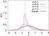Fig. 1 Gaussian and log-normal distribution with zero mean and unit variance, the latter for different α. The larger α is, the stronger the log-normal distribution deviates from the Gaussian.

3.2. Numerical generation of the random fields

In order to evaluate the parameter ς(α), we need to calculate the bispectrum covariance of the Gaussian and the log-normal field, as well as the power spectra. This has been done by numerical simulations: using repeated realisations of the random fields, we can determine their power spectra and bispectra, as well as the covariance of the bispectra from the sample variance among these different realisations. More specifically, we generated realisations of a Gaussian random field with a predefined power spectrum (see below) which uniquely determines its properties. For each realisation of the Gaussian field, we obtained one realisation of a log-normal field applying the transformation (10) to every pixel, for each chosen value of α. In this way, the geometries of the Gaussian and log-normal fields are the same, and the phases of their realisations are the same, which guarantees to minimize sample variance in the comparison carried out in Eq. (9).

A two-dimensional Gaussian random field can be generated easiest in Fourier space using the standard procedure, i.e. assuming periodicity and assigning Fourier coefficients with mean squared amplitude $\mathrm{⟨}\mathrm{|}{\mathit{g}}_{{\ell }}{\mathrm{|}}^{\mathrm{2}}\mathrm{⟩}\mathrm{=}{\left(\frac{\mathrm{\Delta }\mathit{\ell }}{\mathrm{2}\mathit{\pi }}\right)}^{\mathrm{2}}\mathit{P}\mathrm{(}\mathrm{\left|}{\ell }\mathrm{\right|}\mathrm{)}\mathrm{=}{\mathit{\sigma }}_{\mathrm{G}}^{\mathrm{2}}\mathrm{(}\mathrm{\left|}{\ell }\mathrm{\right|}\mathrm{)}\mathit{.}$(15)The variance ${\mathit{\sigma }}_{\mathrm{G}}^{\mathrm{2}}\mathrm{\left(}\mathrm{\right|}{\ell }\mathrm{\left|}\mathrm{\right)}$ of the Gaussian random field $\begin{array}{}{}_{\mathrm{˜}}\\ \mathit{g}\end{array}\mathrm{\left(}{\ell }\mathrm{\right)}$ is uniquely determined by the choice of an input power spectrum P(|ℓ|) and the choice of a smallest wave number Δℓ, or equivalently, the field size Ω. It is needed as input for a Gaussian random number generator (see Galassi et al. 2009), which draws separately the real and imaginary parts of g_ℓ for each wave vector ℓ from a Gaussian distribution with standard deviation ${\mathit{\sigma }}_{\mathrm{G}}\mathrm{\left(}\mathrm{\right|}{\ell }\mathrm{\left|}\mathrm{\right)}\mathrm{\propto }\sqrt{\mathit{P}\mathrm{\left(}\mathrm{\right|}{\ell }\mathrm{\left|}\mathrm{\right)}}$. For our purpose, we choose an input power spectrum with a shape resembling the one of the projected density field (Schneider et al. 1998) $\mathit{P}\mathrm{\left(}\mathit{\ell }\mathrm{\right)}\mathrm{\propto }\mathit{\ell }\mathrm{(}\mathit{\ell }\mathrm{+}{\mathit{\ell }}_{\mathrm{0}}{\mathrm{)}}^{-4}\mathit{,}$(16)with a normalisation that leads to unit variance of g on pixel scale, and we put ℓ₀ = 1000. The size of the field is fixed to Ω = 10° × 10°, leading to a smallest wave number of Δℓ ≈ 36. The field is discretised onto N² = 1024² grid points.

As the log-normal field is obtained from the corresponding Gaussian field by a transformation in real space (see Eq. (10)), the Gaussian field is transformed from Fourier space to real space using the fast Fourier transform algorithm FFTW (see Frigo & Johnson 2005). After the log-normal field is calculated according to Eq. (10), it is then transformed back to Fourier space.

To achieve a good signal-to-noise for the comparison of the bispectrum covariance matrix of the Gaussian with those of the log-normal random fields, it is crucial to generate a large number N_r of realisations of the corresponding field; we choose N_r = 1000. For each field the power spectrum and the bispectrum are computed for each of these N_r realisations and then the average over these N_r power spectra and bispectra is calculated, as well as the variance of the bispectra, which yields an estimate of the bispectrum covariance.

4. Results

4.1. Power spectrum

To determine the range of validity of the Gaussian approximation according to Eq. (9), the measurement of the power spectrum of the Gaussian and of the log-normal fields is necessary. The power spectrum is computed for every realisation of each field as the average of the Fourier coefficients |g_ℓ|² and |L_ℓ|², respectively, over the polar angle of ℓ.

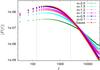Fig. 2 The mean power spectrum, averaged over 1000 realisations, of the Gaussian random field and the mean log-normal power spectrum for different degrees of non-Gaussianity α. The error bars are the standard deviation of the 1000 power spectra divided by $\sqrt{\mathrm{1000}}$.

Figure 2 shows the mean power spectrum obtained by averaging over the 1000 power spectra for each field in the range ℓ ≈ 36−26 000. To determine the bispectrum covariance, the power spectrum and bispectrum are measured in bins equidistant with Δℓ = 110 in the range highlighted in Fig. 2 (ℓ = 145−2455). In the following, we restrict all measurements to the range ℓ = 145−2455, since for substantially larger ℓ, the computing time for the bispectrum becomes quite long.

The power spectra of the Gaussian and the log-normal random field do not differ noticeably for α = 0.1; in fact, these two cannot be distinguished in Fig. 2. However, for α ≥ 0.5, the power spectrum of the log-normal field starts to differ from that of the Gaussian. Given that the log-normal transformation has positive curvature, it increases the amplitude and decreases the width of density peaks. This leads to an increase of power on small scale, as is clearly seen in Fig. 2. Since the variances of all fields are the same on the pixel scale, this increase of power for large ℓ must be compensated by a corresponding decrease of the power for large scales.

4.2. Bispectrum

According to Eq. (1), one way to compute the bispectrum of a random field is to calculate the 3-point correlator in Fourier space and to normalise it afterwards by the corresponding prefactor. We employed such a code, which generates at the beginning of the computational process a list of all Fourier coefficients contained in the different bins defined in Sect. 4.1. For every bin, the code loops over all combinations of the wave vectors ℓ₁, ℓ₂ and ℓ₃ and checks whether the triangle condition is satisfied, i.e., ℓ₁ + ℓ₂ + ℓ₃ = 0. The wave vectors are further constrained to form triangles close to the targeted shape and size, with an allowed deviation of Δℓ_i = 55.

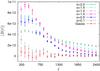Fig. 3 The mean bispectrum per bin for equilateral triangles, averaged over 1000 realisations, of the Gaussian random field and several log-normal fields with different values of the non-Gaussianity parameter α. The error bars are the standard deviation of the 1000 power spectra divided by $\sqrt{\mathrm{1000}}$.

We first restrict our consideration to equilateral triangles, i.e., that all are equal. The mean bispectrum of the 1000 realisations of the Gaussian and log-normal random fields for different values of α is shown in Fig. 3. As expected, the bispectrum of the Gaussian field is compatible with zero within the statistical accuracy of our simulations. The size of the error bars increases towards smaller ℓ due to the smaller number of modes (or available triangles) per ℓ-bin. For the log-normal fields, the bispectrum deviates significantly from zero even for α = 0.1. For small values of α the amplitude of the bispectrum increases with α at all values of ℓ considered. As seen in Fig. 2, for α ≲ 0.5, the power spectra of the log-normal fields are very similar, and therefore the increase of the bispectrum with α shows an increasing degree of non-Gaussianity. For larger values of α, the bispectrum no longer behaves monotonically with α at all ℓ, which is related to the dependence of the power spectrum on α. To leading order, the third-order statistics of a log-normal field is the product of an α-dependent factor describing the degree of non-Gaussianity, and the square of second-order statistics. Hence, the decrease of the bispectrum with α for larger values of α and smaller ℓ reflects the decrease of the power spectrum with α for these ℓ, which results from our normalisation condition. For large ℓ, the bispectrum monotonically increases with α.

4.2.1. The reduced bispectrum – estimating the degree of non-Gaussianity

In order to remove the leading, quadratic dependence of the bispectrum on the power spectrum, we consider the reduced bispectrum, defined as

$\mathit{B}\mathrm{\left(}{\mathit{\ell }}_{\mathrm{1}}\mathit{,}{\mathit{\ell }}_{\mathrm{2}}\mathit{,}{\mathit{\ell }}_{\mathrm{3}}\mathrm{\right)}\mathrm{\left[}\mathit{P}\mathrm{\right(}{\mathit{\ell }}_{\mathrm{1}}\mathrm{\left)}\mathit{P}\mathrm{\right(}{\mathit{\ell }}_{\mathrm{2}}\mathrm{)}\mathrm{+}\mathit{P}\mathrm{(}{\mathit{\ell }}_{\mathrm{1}}\mathrm{\left)}\mathit{P}\mathrm{\right(}{\mathit{\ell }}_{\mathrm{3}}\mathrm{)}\mathrm{+}\mathit{P}\mathrm{(}{\mathit{\ell }}_{\mathrm{2}}\mathrm{\left)}\mathit{P}\mathrm{\right(}{\mathit{\ell }}_{\mathrm{3}}\mathrm{)}{\mathrm{]}}^{-1}\mathit{,}$which for equilateral triangles reduces to B(ℓ)/3P²(ℓ). This reduced bispectrum is shown for different α in Fig. 4. As expected, its amplitude grows with increasing α; for α = 1.5 it is approximately five times larger than for α = 0.1. Additionally, the reduced bispectrum increases with ℓ, indicating a larger degree of non-Gaussianity on smaller scales.

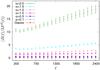Fig. 4 The reduced bispectrum B(ℓ)/3P2(ℓ) for a Gaussian and several log-normal random fields with different α. The error bars are calculated by Gaussian error propagation.

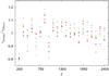Fig. 5 The relation between the theoretically calculated geometrical factor and the numerically computed geometrical factor γnum/γtheo for seven sets of 1000 realisations of a Gaussian random field. For clarity the error bars are not plotted.

4.3. Bispectrum covariance

4.3.1. Accuracy for the Gaussian case

Before testing the range of validity of the Gaussian approximation for the bispectrum covariance of non-Gaussian fields, it is reasonable to first probe the accuracy of the Gaussian approximation for a purely Gaussian random field. For this, we calculate the ratio of the numerically determined bispectrum covariance and third-order products of the power spectrum, to obtain the geometrical factor γ_num from the simulations, which is then compared to the expected value γ_theo given by Eq. (5). The value of γ_num has been determined for seven sets of 1000 realisations individually; the ratio γ_num/γ_theo for these seven sets is shown in Fig. 5. The ratio fluctuates around one, with higher fluctuations for smaller wave numbers ℓ, which is due to the fact that the results on large scales are obtained by averaging over fewer triangles than on small scales. Only at the smallest value of ℓ considered do we see a significant deviation of this ratio from unity. This deviation is not surprising, given the various approximations that were made for deriving Eq. (4), the most important of which is that the spatial scale is much smaller than the size of the field, so that edge effects can be neglected. For ℓ = 200, corresponding to about 1deg, this assumption is no longer fully justified. However, for larger values of ℓ we conclude that the analytical expression for the geometrical factor is accurate.

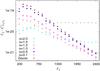Fig. 6 The diagonal elements (ℓ1 = ℓ2) of the Gaussian covariance matrix compared to the diagonal elements of the log-normal covariance matrix for different degrees of non-Gaussianity α. For clarity, the diagonal elements are multiplied by the factor ℓ1, and the error bars are not plotted.

4.3.2. Diagonal elements

The Gaussian approximation for the bispectrum covariance says that for equilateral triangles, ${\mathit{C}}_{\mathit{\ell ̅}\mathrm{1}\mathit{\ell ̅}\mathrm{2}}\mathrm{\equiv }\mathrm{Cov}\left(\mathit{B̂}\mathrm{\left(}\mathit{\ell ̅}\mathrm{1}\mathit{,}\mathit{\ell ̅}\mathrm{1}\mathit{,}\mathit{\ell ̅}\mathrm{1}\mathrm{\right)}\mathit{,}\hspace{0.17em}\mathit{B̂}\mathrm{\left(}\mathit{\ell ̅}\mathrm{2}\mathit{,}\mathit{\ell ̅}\mathrm{2}\mathit{,}\mathit{\ell ̅}\mathrm{2}\mathrm{\right)}\right)\mathrm{=}\mathit{\gamma }{\mathit{P}}^{\mathrm{3}}\mathrm{\left(}\mathit{\ell ̅}\mathrm{1}\mathrm{\right)}{\mathit{\delta }}_{\mathit{\ell ̅}\mathrm{1}\mathit{\ell ̅}\mathrm{2}}\mathit{,}$(17)i.e., that the off-diagonal elements of C_ℓ1ℓ2 are zero, and that the diagonal elements follow the Gaussian behaviour. Here, we first study the latter, and show the diagonal elements in Fig. 6. For α ≲ 0.5, the diagonal elements for the log-normal case show no significant difference from the Gaussian case, whereas for α ≳ 0.5 the amplitude of the diagonal elements of the log-normal covariance matrix decreases in comparison to the Gaussian covariance matrix, reflecting the decrease of the power spectrum with α across the ℓ range considered. For large values of α, C_ℓℓ increases again, due to the larger degree of non-Gaussianity, where the higher-order terms of Eq. (4), unaccounted for in the Gaussian approximation, start dominating the behaviour of the covariance matrix.

To remove the dependence of the covariance from the power spectrum, we consider the aberration parameter ς(α) defined in Eq. (9). This is shown in Fig. 7 for several relatively large values of α. For this figure, we study the aberration parameter down to roughly eight times the pixel scale. This figure indicates that ς is of order unity for α ≲ 1.2, but strongly increases for larger values of α, indicating a clear breakdown of the Gaussian approximation. To study in more detail the transition to this breakdown, we show in Fig. 8 the behaviour of ς with ℓ for several smaller values of α. This figure indicates that for α = 0.5, ς ≈ 1 within the statistical accuracy, and that ς ≈ 1.1 for α = 1.0. For α = 1.2, the deviations are already several tens of percent, and clearly increase towards larger ℓ. Hence we conclude that the diagonal elements of the covariance are well described by the Gaussian approximation for α ≲ 0.5, on the scales probed, and that the deviation from the Gaussian approximation are confined to less than 10% for α ≲ 1.

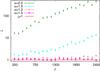Fig. 7 Aberration parameter ς for large degrees of non-Gaussianity α. The error bars are computed by Gaussian error propagation using $\mathrm{\Delta }\mathrm{Cov}\mathrm{=}{\mathit{C}}_{\mathit{ij}}\sqrt{\mathrm{2}\mathit{/}\mathrm{(}\mathrm{1000}\mathrm{-}\mathrm{1}\mathrm{)}}$.

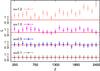Fig. 8 Aberration parameter ς for small degrees of non-Gaussianity α.

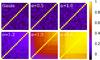Fig. 9 Gaussian and log-normal correlation matrices for different α. The wave numbers ℓ1 and ℓ2 rise for each panel from the left lower corner to the right upper corner.

4.3.3. Off-diagonal elements

The validity of the Gaussian approximation furthermore requires the vanishing of the off-diagonal elements of the covariance matrices. We define the correlation coefficient ${\mathrm{r}}_{{\mathit{\ell }}_{\mathrm{1}}{\mathit{\ell }}_{\mathrm{2}}}\mathrm{=}{\mathit{C}}_{{\mathit{\ell }}_{\mathrm{1}}{\mathit{\ell }}_{\mathrm{2}}}\mathit{/}\sqrt{{\mathit{C}}_{{\mathit{\ell }}_{\mathrm{1}}{\mathit{\ell }}_{\mathrm{1}}}{\mathit{C}}_{{\mathit{\ell }}_{\mathrm{2}}{\mathit{\ell }}_{\mathrm{2}}}}\mathit{,}$(18)which by definition is unity for the diagonal elements, and plot this in Fig. 9 for different values of α. As expected, the off-diagonal elements are compatible with zero for the Gaussian case, and are also very small for the log-normal fields with α ≲ 1. For larger values of α, the off-diagonal elements of the correlation coefficient become significantly non-zero, clearly indicating the breakdown of the Gaussian approximation. The amplitude of the off-diagonal elements increases with ℓ₁ and ℓ₂, i.e., for smaller scales where the non-Gaussianity of the fields is stronger. To show this behaviour in more detail, Fig. 10 shows the correlation coefficient r_ℓ1ℓ2 as a function of the wave number ℓ₁ for various values of ℓ₂. For α = 1.0 the off-diagonal elements are still almost zero, but increase for α > 1.0 with large ℓ₁ and ℓ₂.

Combining the results from studying the diagonal and non-diagonal elements of the bispectrum covariance for equilateral triangles, we conclude that the Gaussian approximation provides, on the scales considered (down to eight times the pixel scale), an accurate description of the bispectrum covariance for degrees of non-Gaussianity corresponding to α ≲ 0.5, and a very reasonable approximation even for α ≲ 1. For larger degrees of non-Gaussianity, the Gaussian approximation starts to break down, and higher-order terms become important for calculating the bispectrum covariance. In general, the Gaussian approximation works better for large scales than for small scales, as non-Gaussianity contributes more on small scales and therefore the Gaussian approximation should be worse for this case.

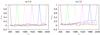
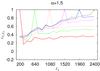Fig. 10 The correlation coefficient rℓ1ℓ2 of the log-normal covariance matrix as a function of the wave vector ℓ1 for various values of ℓ2 for different α. The value of ℓ2 corresponding to each curve can be read off from the point where the curve attains the value 1.

4.3.4. Degree of non-Gaussianity for cosmic shear fields

In order to relate our results to future studies of third-order statistics of cosmic shear fields, we need to obtain an estimate of the degree of non-Gaussianity, here parametrised in terms of α, of realistic shear (or convergence) fields. As shown by Taruya et al. (2002) and Hilbert et al. (2011), the cosmic shear convergence distribution is rather well described by a log-normal; from their results we can estimate characteristic values of α.

A comparison of the probability distributions used in Taruya et al. (2002) and in Hilbert et al. (2011) with the one used for our investigations (see Eq. (14)) shows that the probability distributions are equivalent, except that we have fixed A to get unit variance for the log-normal field. The convergence field κ of Taruya et al. (2002) and Hilbert et al. (2011) corresponds to the log-normal field L used in this paper. Furthermore, the parameter |κ_min| or κ₀ corresponds to the parameter A, which was introduced in Sect. 3.1. Finally, their quantity σ is equivalent to the non-Gaussianity parameter α. Thus, the degree of non-Gaussianity α of the convergence field κ can directly be estimated from the σ computed by Taruya et al. (2002) and Hilbert et al. (2011).

For a source redshift of z = 1, a smoothing angle of $\mathit{\theta }\mathrm{=}\mathrm{4}\stackrel{\mathrm{\prime }}{.}\mathrm{0}$ and a LCDM-model one can compute from Taruya et al. (2002) that the degree of non-Gaussianity of the convergence field κ corresponds to α ≈ 0.437. The result we obtain from Hilbert et al. (2011) is α ≈ 0.658 for unsmoothed fields. Here the smoothing is implicitly determined by the parameters in the cosmological simulation, roughly to  ~3′′.5. Evidently, the value of α is not a strong function of smoothing scale here. In either case, the non-Gaussianity of cosmic shear convergence fields are estimated to correspond to α < 1, from which we conclude that the Gaussian approximation for the covariance bispectrum is likely to be applicable in cosmic shear studies, at least down to angular scales of  ~30′′.

4.4. Non-equilateral triangles

The results shown so far are based on calculations of the bispectrum for equilateral triangles, to have just a single parameter. However, to get a more complete view on the range of applicability of the Gaussian approximation, the bispectrum must in principle be calculated for all possible triangle shapes. Here, we will consider two more shapes of triangles; for the first case, which we term “truncated triangles”, we set ℓ₁ = ℓ₂ = ℓ, ℓ₃ = ℓ/3, whereas in the second case, denoted “sharp triangles”, we set ℓ₁ = ℓ₂ = ℓ, ℓ₃ = 1.5ℓ. For both cases, we calculate the covariance of the bispectrum, as was done in the equilateral case before.

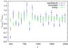Fig. 11 The relation between the theoretically calculated geometrical factor and the numerically computed geometrical factor γnum/γtheo for one Gaussian random field (with 1000 realisations) for different triangle shapes, all of which have ℓ1 = ℓ2 = ℓ: equilateral (ℓ3 = ℓ), truncated (ℓ3 = ℓ/3) and sharp (ℓ3 = 1.5ℓ) triangles. Error bars are computed by Gaussian error propagation.

In Fig. 11, we first check the accuracy of the analytical estimate for the Gaussian case, i.e., the ratio γ_num/γ_theo is shown for equilateral triangles (black), truncated triangles (blue) and sharp triangles (green). As seen before, the Gaussian approximation provides a good description of the bispectrum covariance in the case of Gaussian fields. There is a larger scatter around 1 for truncated triangles, and a smaller scatter for sharp triangles, than for equilateral triangles. This is due to the fact that truncated triangles probe the field properties on larger angular scales than equilateral triangles; the opposite is true for sharp triangles. Accordingly there are fewer (more) triangles to average over for truncated (sharp) triangles than for equilateral ones.

For a log-normal field with α = 0.5, we plot the aberration parameter ς in Fig. 12 for the three different kinds of triangles. As can be seen, there is no significant difference for truncated and sharp triangles to the results obtained for equilateral triangles. This simple example thus indicates that the Gaussian approximation for the bispectrum covariance also holds for other triangle shapes. We therefore conclude that the Gaussian approximation can be applied for log-normal fields with a degree of non-Gaussianity α ≤ 0.5. In combination with what was said above, this implies that for applications to cosmic shear, the Gaussian approximation for the bispectrum covariance is sufficiently accurate for the range of scales studied.

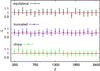Fig. 12 The aberration parameter ς(α = 0.5) for equilateral, truncated and sharp triangles.

5. Summary and conclusion

In this paper we studied the range of applicability of the Gaussian approximation for the bispectrum covariance, as derived by Joachimi et al. (2009), for non-Gaussian fields. We chose log-normal random fields as representative for non-Gaussian fields motivated by the fact that the one-dimensional probability density function of the density fluctuations and the one-dimensional probability density function of the cosmic shear convergence field as well as the covariance of the power spectrum of cosmic shear fields are well described by the log-normal ansatz. However, it has not been shown so far how well higher-order statisics of cosmic fields are described by this ansatz. Furthermore, the log-normal is not completely determined by its moments. Thus the log-normal approach can only be seen as a first step to describe the present non-Gaussian Universe.

Our study is based on numerical simulations of Gaussian and log-normal fields with different degrees α of non-Gaussianity. Using 1000 realisations of these fields, their bispectrum was calculated, and the bispectrum covariance was estimated from the sample variance.

In our simulations, α is a non-Gaussianity parameter of the transformation (10). This formula is applied to the pixel values in realisations of Gaussian fields on a grid. For convenience, the pixel value variance was chosen to be unity in the Gaussian and in the log-normal case. We could as well have chosen the pixel variance in the Gaussian and non-Gaussian field to be σ² without changing the essential results of this paper because this would have just modified A in Eq. (12). This would have rescaled the entire field by a mere constant factor, leaving the skewness (Appendix) untouched.

The following conclusions are drawn for angular scales down to approximately eight times the pixel scale. We have shown that the bispectrum covariance remains almost diagonal, as long as α ≲ 1. Furthermore, the deviation of the diagonal elements from those predicted by the Gaussian approximation are negligible for α ≲ 0.5, and below 10% for α ≲ 1. From simulations of convergence fields in weak lensing shown in Taruya et al. (2002) and Hilbert et al. (2011), we found that realistic values of α are not larger than  ~0.7 on angular scales of about 4′′; hence, the Gaussian approximation is expected to yield an accurate description of the bispectrum covariance – which is fortunate, given the complexity of the full expression of this covariance.

Whereas the results depend on the assumed statistical properties of the non-Gaussian field – here assumed to be log-normal – as well as on the shape of the power spectrum, which we chose somewhat arbitrarily but resembling the shape of the projected density field, we expect that the accuracy of the Gaussian approximation for the bispectrum covariance depends predominantly on the degree of non-Gaussianity (here parametrised by α, but we could equivalently use the skewness of the field – see Appendix).

Acknowledgments

We thank Benjamin Joachimi, Jan Hartlap, Xun Shi and Stefan Hilbert for many fruitful discussions and their help in this project. This work was supported by the Deutsche Forschungsgemeinschaft in the framework of the Collaborative Research Center TR33 “The Dark Universe”.

References

Appendix A: Skewness of the log-normal field

Besides the mean and the variance, higher-order moments of the log-normal random field L can be calculated easily, for example the third-order moment 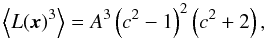$\mathrm{⟨}\mathit{L}\mathrm{(}{x}{\mathrm{)}}^{\mathrm{3}}\mathrm{⟩}\mathrm{=}{\mathit{A}}^{\mathrm{3}}{\mathrm{(}{\mathit{c}}^{\mathrm{2}}\mathrm{-}{\mathrm{1}}^{\mathrm{)}}}^{\mathrm{2}}\mathrm{(}{\mathit{c}}^{\mathrm{2}}\mathrm{+}{\mathrm{2}}^{\mathrm{)}}\mathit{,}$(A.1)which is of special interest as it is related to the skewness parameter Γ⁽³⁾ by: 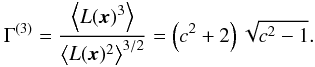${\mathrm{\Gamma }}^{\mathrm{\left(}\mathrm{3}\mathrm{\right)}}\mathrm{=}\frac{\mathrm{⟨}\mathit{L}\mathrm{(}{x}{\mathrm{)}}^{\mathrm{3}}\mathrm{⟩}}{{⟨\mathit{L}\mathrm{(}{x}{\mathrm{)}}^{\mathrm{2}}⟩}^{\mathrm{3}\mathit{/}\mathrm{2}}}\mathrm{=}\mathrm{(}{\mathit{c}}^{\mathrm{2}}\mathrm{+}{\mathrm{2}}^{\mathrm{)}}\sqrt{{\mathit{c}}^{\mathrm{2}}\mathrm{-}\mathrm{1}}\mathit{.}$(A.2)As the skewness depends ultimately only on α, the latter can be regarded as to set the skewness of the log-normal field L(x), which can also be visualised by the Taylor expansion of Eq. (A.2), 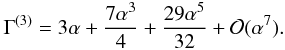${\mathrm{\Gamma }}^{\mathrm{\left(}\mathrm{3}\mathrm{\right)}}\mathrm{=}\mathrm{3}\mathit{\alpha }\mathrm{+}\frac{\mathrm{7}{\mathit{\alpha }}^{\mathrm{3}}}{\mathrm{4}}\mathrm{+}\frac{\mathrm{29}{\mathit{\alpha }}^{\mathrm{5}}}{\mathrm{32}}\mathrm{+}\mathrm{𝒪}\mathrm{\left(}{\mathit{\alpha }}^{\mathrm{7}}\mathrm{\right)}\mathit{.}$(A.3)

All Figures

	Fig. 1 Gaussian and log-normal distribution with zero mean and unit variance, the latter for different α. The larger α is, the stronger the log-normal distribution deviates from the Gaussian.
In the text

	Fig. 2 The mean power spectrum, averaged over 1000 realisations, of the Gaussian random field and the mean log-normal power spectrum for different degrees of non-Gaussianity α. The error bars are the standard deviation of the 1000 power spectra divided by $\sqrt{\mathrm{1000}}$.
In the text

	Fig. 3 The mean bispectrum per bin for equilateral triangles, averaged over 1000 realisations, of the Gaussian random field and several log-normal fields with different values of the non-Gaussianity parameter α. The error bars are the standard deviation of the 1000 power spectra divided by $\sqrt{\mathrm{1000}}$.
In the text

	Fig. 4 The reduced bispectrum B(ℓ)/3P2(ℓ) for a Gaussian and several log-normal random fields with different α. The error bars are calculated by Gaussian error propagation.
In the text

	Fig. 5 The relation between the theoretically calculated geometrical factor and the numerically computed geometrical factor γnum/γtheo for seven sets of 1000 realisations of a Gaussian random field. For clarity the error bars are not plotted.
In the text

	Fig. 6 The diagonal elements (ℓ1 = ℓ2) of the Gaussian covariance matrix compared to the diagonal elements of the log-normal covariance matrix for different degrees of non-Gaussianity α. For clarity, the diagonal elements are multiplied by the factor ℓ1, and the error bars are not plotted.
In the text

	Fig. 7 Aberration parameter ς for large degrees of non-Gaussianity α. The error bars are computed by Gaussian error propagation using $\mathrm{\Delta }\mathrm{Cov}\mathrm{=}{\mathit{C}}_{\mathit{ij}}\sqrt{\mathrm{2}\mathit{/}\mathrm{(}\mathrm{1000}\mathrm{-}\mathrm{1}\mathrm{)}}$.
In the text

	Fig. 8 Aberration parameter ς for small degrees of non-Gaussianity α.
In the text

	Fig. 9 Gaussian and log-normal correlation matrices for different α. The wave numbers ℓ1 and ℓ2 rise for each panel from the left lower corner to the right upper corner.
In the text

In the text

	Fig. 10 The correlation coefficient rℓ1ℓ2 of the log-normal covariance matrix as a function of the wave vector ℓ1 for various values of ℓ2 for different α. The value of ℓ2 corresponding to each curve can be read off from the point where the curve attains the value 1.
In the text

	Fig. 11 The relation between the theoretically calculated geometrical factor and the numerically computed geometrical factor γnum/γtheo for one Gaussian random field (with 1000 realisations) for different triangle shapes, all of which have ℓ1 = ℓ2 = ℓ: equilateral (ℓ3 = ℓ), truncated (ℓ3 = ℓ/3) and sharp (ℓ3 = 1.5ℓ) triangles. Error bars are computed by Gaussian error propagation.
In the text

	Fig. 12 The aberration parameter ς(α = 0.5) for equilateral, truncated and sharp triangles.
In the text

References

- Bernardeau, F., Mellier, Y., & van Waerbeke, L. 2002, A&A, 389, L28 [Google Scholar]
- Carron, J., & Neyrinck, M. C. 2012, ApJ, accepted [arXiv:1201.1444] [Google Scholar]
- Coles, P., & Jones, B. 1991, MNRAS, 248, 1 [NASA ADS] [CrossRef] [Google Scholar]
- Frigo, M., & Johnson, S. G. 2005, Proc. IEEE 93, special issue on Program Generation, Optimization, and Platform Adaptation, 216 [Google Scholar]
- Galassi, M., Davies, J., Theiler, J., et al. 2009, GNU Scientific Library Reference Manual, third edition (Network Theory Ltd.) [Google Scholar]
- Hilbert, S., Hartlap, J., & Schneider, P. 2011, A&A, 536, A85 [NASA ADS] [CrossRef] [EDP Sciences] [Google Scholar]
- Hu, W. 2000, Phys. Rev. D, 62, 043007 [NASA ADS] [CrossRef] [Google Scholar]
- Huterer, D., Takada, M., Bernstein, G., & Jain, B. 2006, MNRAS, 366, 101 [NASA ADS] [CrossRef] [Google Scholar]
- Jarvis, M., Bernstein, G., & Jain, B. 2004, MNRAS, 352, 338 [NASA ADS] [CrossRef] [Google Scholar]
- Joachimi, B., Shi, X., & Schneider, P. 2009, A&A, 508, 1193 [NASA ADS] [CrossRef] [EDP Sciences] [Google Scholar]
- Kayo, I., Taruya, A., & Suto, Y. 2001, ApJ, 561, 22 [NASA ADS] [CrossRef] [Google Scholar]
- Kilbinger, M., & Schneider, P. 2005, A&A, 442, 69 [NASA ADS] [CrossRef] [EDP Sciences] [Google Scholar]
- Peacock, J. A., & Dodds, S. J. 1996, MNRAS, 280, L19 [NASA ADS] [CrossRef] [Google Scholar]
- Pen, U.-L., Zhang, T., van Waerbeke, L., et al. 2003, ApJ, 592, 664 [NASA ADS] [CrossRef] [Google Scholar]
- Schneider, P. 2006, in Saas-Fee Advanced Course 33: Gravitational Lensing: Strong, Weak and Micro, ed. G. Meylan, P. Jetzer, P. North, P. Schneider, C. S. Kochanek, & J. Wambsganss, 1 [Google Scholar]
- Schneider, P., van Waerbeke, L., Jain, B., & Kruse, G. 1998, MNRAS, 296, 873 [NASA ADS] [CrossRef] [Google Scholar]
- Scoccimarro, R., & Couchman, H. M. P. 2001, MNRAS, 325, 1312 [NASA ADS] [CrossRef] [Google Scholar]
- Semboloni, E., Schrabback, T., van Waerbeke, L., et al. 2011, MNRAS, 410, 143 [NASA ADS] [CrossRef] [Google Scholar]
- Shi, X., Joachimi, B., & Schneider, P. 2010, A&A, 523, A60 [NASA ADS] [CrossRef] [EDP Sciences] [Google Scholar]
- Smith, R. E., Peacock, J. A., Jenkins, A., et al. 2003, MNRAS, 341, 1311 [NASA ADS] [CrossRef] [Google Scholar]
- Takada, M., & Jain, B. 2004, MNRAS, 348, 897 [NASA ADS] [CrossRef] [Google Scholar]
- Taruya, A., Takada, M., Hamana, T., Kayo, I., & Futamase, T. 2002, ApJ, 571, 638 [NASA ADS] [CrossRef] [Google Scholar]