| Issue |
A&A
Volume 543, July 2012
|
|
|---|---|---|
| Article Number | A42 | |
| Number of page(s) | 9 | |
| Section | Astronomical instrumentation | |
| DOI | https://doi.org/10.1051/0004-6361/201117554 | |
| Published online | 25 June 2012 | |
Strategies for the deconvolution of hypertelescope images
1 Université de Nice Sophia-Antipolis, Centre National de la Recherche Scientifique, Observatoire de la Côte d’Azur, UMR 7293 Lagrange, Parc Valrose, 06108 Nice, France
e-mail: This email address is being protected from spambots. You need JavaScript enabled to view it.
2 Princeton University, Mechanical & Aerospace Engineering, Olden street, Princeton, 08544 NJ, USA
e-mail: This email address is being protected from spambots. You need JavaScript enabled to view it.
This email address is being protected from spambots. You need JavaScript enabled to view it.
This email address is being protected from spambots. You need JavaScript enabled to view it.
Received: 24 June 2011
Accepted: 24 April 2012
Abstract
Aims. We study the possibility of deconvolving hypertelescope images and propose a procedure that can be used provided that the densification factor is small enough to make the process reversible.
Methods. We present the simulation of hypertelescope images for an array of cophased densified apertures. We distinguish between two types of aperture densification, one called FAD (full aperture densification) corresponding to Labeyrie’s original technique, and the other FSD (full spectrum densification) corresponding to a densification factor twice as low. Images are compared to the Fizeau mode. A single image of the observed object is obtained in the hypertelescope modes, while in the Fizeau mode the response produces an ensemble of replicas of the object. Simulations are performed for noiseless images and in a photodetection regime. Assuming first that the point spread function (PSF) does not change much over the object extent, we use two classical techniques to deconvolve the images, namely the Richardson-Lucy and image space reconstruction algorithms.
Results. Both algorithms fail to achieve satisfying results. We interpret this as meaning that it is inappropriate to deconvolve a relation that is not a convolution, even if the variation in the PSF is very small across the object extent. We propose instead the application of a redilution to the densified image prior to its deconvolution, i.e. to recover an image similar to the Fizeau observation. This inverse operation is possible only when the rate of densification is no more than in the FSD case. This being done, the deconvolution algorithms become efficient. The deconvolution brings together the replicas into a single high-quality image of the object. This is heuristically explained as an inpainting of the Fourier plane. This procedure makes it possible to obtain improved images while retaining the benefits of hypertelescopes for image acquisition consisting of detectors with a small number of pixels.
Key words: instrumentation: high angular resolution / instrumentation: interferometers / techniques: high angular resolution / techniques: interferometric
© ESO, 2012
1. Introduction
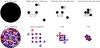 |
Fig. 1 Top: from left to right: a monolithic giant aperture (the so-called meta-telescope), a diluted array of four telescopes in Fizeau mode and in the two hypertelescope modes FSD and FAD. Bottom: phase of the image transform for the test object, which clearly illustrates it visible the aliasing effect in the FAD mode. This aliasing makes it impossible to recover the Fizeau spectrum in the FAD mode, while the inverse operation remains possible in the FSD mode. |
Since the pioneering observations of Michelson (1920), optical interferometers have been used to obtain high angular information about stellar structures. This advancement has taken a long time from the early measurement of Betelgeuse’s diameter by Michelson & Pease (1921), to the use of two coherent telescopes (Labeyrie 1975; Mourard et al. 1994) and the development of stellar interferometers such as CHARA (ten Brummelaar et al. 2005; Mourard et al. 2009) and VLTI (Ohnaka et al. 2011).
The achievements of optical interferometers cannot yet be compared with the imaging capabilities of radiotelescopes, although this may be possible in the foreseeable future. For ground-based instruments, the observations suffer from the imperfect correction of the effect for atmospheric turbulence, but progress in adaptive optics, combined with the use of phase closure techniques, can solve most of this problem.
The array configuration, as well as the number and sizes of the telescopes, is a key issue in interferometric imaging (Kopilovich & Sodin 2001). The point spread function (PSF) is not a compact spot such as the Airy disk, and can have a structure that is apparently chaotic. The resulting image is the so-called dirty image, and a post-processing is mandatory to recover a usable image.
Labeyrie (1996) proposed to overcome this problem using a densification of the aperture, so that the final aperture seen at the array final focus resembled as much as possible a monolithic aperture. The result is a snapshot image that can be directly used for astrophysical studies. He defined hypertelescope to be the association of diluted apertures and densification. We use this term in the present paper without specifying either the configuration of the apertures or the degree of densification.
In the present paper, we will study the possibility of an improvement of these snapshot images by means of deconvolution. Since the concept of an hypertelescope involves direct imaging, we do not consider in the present study the super-synthesis possibility, and the simulations that we present here are limited to the specific case in which a single configuration of many diluted apertures can make an image scientifically exploitable. Moreover, we restrict our analysis to the perfect case of a coherent array of telescopes in space (i.e. no atmospheric turbulence) for which a point spread function (PSF) is available. We have therefore the conditions for which classic deconvolution algorithms such as the Richardson-Lucy algorithm (RLA) or the iterative space reconstruction algorithm (ISRA) can be used directly, without having to consider more specific algorithms such as those used in Thiebaut & Giovannelli (2010).
The paper is organized as follows. The principle of the simulation of hypertelescope images is described in Sect. 2, where it is illustrated for a diluted array of 25 non-redundant apertures observing an extended object. Noisy observations are simulated assuming Poisson noise. Assuming a convolution relationship to the hypertelescope image, two deconvolution techniques, namely RLA and ISRA, are applied to the simulated images in Sect. 3. The results are disappointing, but the deconvolution procedure is then applied more successfully to images obtained after rediluting the MTF, when the rate of densification is not too strong and allows this inverse operation. A discussion is given in the last section.
2. Simulation of hypertelescope images
2.1. Principle of the hypertelescopes
In the particular case where the array takes the form of a two-dimensional highly diluted grid, the raw focal plane image in the basic Fizeau configuration shows a large number of replicas of the object, and the use of an hypertelescope makes it possible to bring together every replica in a single image. This has the advantage of requiring detectors with smaller numbers of pixels. Moreover, the photons are not randomly dispersed over the multiple replicas of the astrophysical image of interest, as in the case of the Fizeau mode.
The hypertelescope concept proposed by Labeyrie (1996) consists in an operation of densification of the telescope array that brings the apertures closer to each other, using for example the periscopic principle of Michelson. In this operation, the pattern of sub-pupil centers must remain identical in the entrance and exit pupils, to an homothetic transformation. An equivalent result can be obtained by applying a magnification of the elementary apertures by means of inverted Galilean telescopes. In the following, we consider the periscope assembly because it is more suitable for a numerical simulation. A change of scale in the system allows us to switch from the periscopic mode to the Galilean one, although this requires an interpolation of the data.
Apertures may differ from one another, but for simplicity we consider here K identical elementary circular apertures of diameter D and transmissions P0(r), centered at positions rk = (xk,yk). For an incoming wave Ψ0(r), the telescope, assumed to be perfect, transmits a wave Ψ(r) that is restricted to the K apertures and can be written as 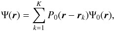 (1)where the mathematical condition on the rk is the non-overlapping of apertures. For hypertelescopes, we can follow the approach of Tallon & Tallon-Bosc (1992) and consider that the wave is modified so that the wavefront that arrives on the elementary aperture located at the position rk is translated as a whole to a new position
  , with the same condition of non-overlapping apertures. The wave corresponding to the densified aperture seen from the final focus appears as the function Ψ′(r) of the form
 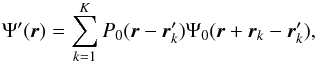 (2)where
  are the new positions of the centers of the apertures and the set of positions form an homothetic smaller image of the rk. It is important to emphasize that the waves in the apertures
  are those collected by the direct aperture P0(r − rk).
The densification factor defined by Labeyrie (1996) is the ratio γ = d/d′ between the distances of the centers before and after this operation. Different factors can be used. If all apertures are identical circular apertures of diameter D, and if the minimal distance between their centers is d, then γM = d/D is the maximal value of γ, which corresponds to d′ = D. This thus means that the densification ensures that some of the apertures are next to each other. We refer to this mode as full aperture densification (FAD).
As discussed by Aime (2008) and recalled in the present paper, the FAD mode produces an overlapping of different spatial frequencies in the final densified image spectrum and the effect is similar to aliasing. This led us to consider another mode of densification that maximizes the factor of densification while preventing any overlapping of the spatial frequencies in the densified image spectrum. We denote this as full spectrum densification (FSD), which corresponds to γ = γM/2. These densifications, which are described in greater detail in the next paragraph, are illustrated in Fig. 1 for a non-redundant array of four apertures.
The formulation of the image formation process with a hypertelescope in the Michelson mode has been studied in several publications after being initially proposed by Labeyrie (1996). As a result of the transformation, the PSF depends on the position of the point source on the sky, as described by Labeyrie (2007), Lardière et al. (2007), Patru et al. (2008), and Patru et al. (2009). From a numerical point of view, this makes it difficult to simulate the final image because the relation of the convolution relationship between the object and the image must be replaced by a Fredholm equation of the first kind in which the kernel is no longer space-invariant.
The numerical implementation of the two-dimensional Fredholm equation is somewhat heavy. Thankfully, there is a more effective way of simulating hypertelescope images. The procedure was described by Aime (2008), and it makes use of the approach of Tallon & Tallon-Bosc (1992). These latter authors developed a complete analysis of densification in their study of the object-image relationship in Michelson stellar interferometry. Their main result is that in the Michelson configuration the part of the Fourier plane transmitted by a pair of telescopes around the frequency ukl = (rk − rl)/λ is shifted as a whole to a lower frequency  , without any modification of the frequency transmission in neither modulus or phase. Since with a hypertelescope, the transformation of the centers of transmission domains is homothetic, for all k and l, we have
  .
.
Using this property, the procedure to simulate an hypertelescope image may be seen as a simple modification of the linear filtering process used to simulate an image with a diluted aperture array. In the Fizeau mode, the image I(α) observed in the focal plane of an ideal cophased array is simulated by taking the inverse Fourier transform ![Mathematical equation: \begin{equation} \label{EqNew3} I(\boldsymbol \alpha)=\mathcal{F}^{-1}\left[ \hat{I}(\boldsymbol u)\right]=\mathcal{F}^{-1}\left[ T(\boldsymbol u) \hat{O}(\boldsymbol u)\right]. \end{equation}](/articles/aa/full_html/2012/07/aa17554-11/aa17554-11-eq27.png) (3)In that relation, Ô(u) is the two-dimensional Fourier transform of the geometrically perfect image of the object O(α), and T(u) is the optical transfer function of the aperture array
(3)In that relation, Ô(u) is the two-dimensional Fourier transform of the geometrically perfect image of the object O(α), and T(u) is the optical transfer function of the aperture array 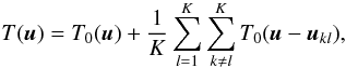 (4)where T0(u) is the MTF of an elementary aperture and the ukl are the position differences between the rk, expressed in units of wavelength, as already indicated.
The simulation of images obtained with a perfect hypertelescope is easily performed by modifying Î(u) of the Fizeau mode into a new value Î′(u) that corresponds to the densified mode. Rewriting Eq. (12) of Tallon & Tallon-Bosc (1992),  can be written as
 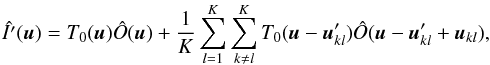 (5)The term
  represents a translation in the frequency plane. We note that making
  , we have
  and recover the filtering relationship given in the former equations. The hypertelescope image I′(α) is obtained as the inverse Fourier transform
 ![Mathematical equation: \begin{equation} \label{EqNew6} I'(\boldsymbol \alpha)=\mathcal{F}^{-1}[\hat{I'}(\boldsymbol u)]. \end{equation}](/articles/aa/full_html/2012/07/aa17554-11/aa17554-11-eq42.png) (6)An illustration of the operation that transforms Î(u) into
(6)An illustration of the operation that transforms Î(u) into  is given in Fig. 1. The array of 4 telescopes provides a sampling of 13 zones in the image transform plane, which are called initial sampling in the figure. The figure illustrates the two modes of densification FAD and FSD already presented. The four top figures show the pupil configurations in both the initial pupil plane and re-imaged pupil planes. The four bottom figures indicate how the spatial frequencies are sampled and manipulated, and the illustration is given for the phase of the transform, and an astronomical test object.
We now examine in more detail the two cases of FAD and FSD. In the Fourier plane, the MTF is given by the aperture autocorrelation function. Apertures separated by a distance of d give frequency transmissions at 0 and ± d/λ. The MTF T0(u) of elementary apertures spreads over a frequency area of diameter 2D/λ. In the FAD mode, making d′ = D will produce a strong overlapping in the MTF, as illustrated in Fig. 1. In contrast, the FSD is the strongest possible densification that preserves the spectrum from overlapping (because d′ = 2D). This can also be analyzed using Eq. (5). The support of T0(u) is a circle of diameter 2D/λ. To avoid any overlap between different  , it is mandatory that distances between different
  be larger than D/λ.
In conclusion to this section, we wish to emphasize that a densification rate no stronger than in the FSD mode is mandatory if the initial Fizeau mode is to be recovered. This inverse operation is impossible in the fully densified FAD mode that was originally proposed by Labeyrie (1996), and we will demonstrate in the following sections that this prevents any improvement in the hypertelescope image quality.
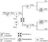 |
Fig. 2 Block-diagram of the numerical simulation giving the interferometric and hypertelescope images at high light level (I(α) and I′(α)) and in photodetection mode (Ip(α) and |

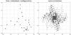 |
Fig. 3 Example of positions for a configuration of 25 point-like non-redundant apertures (left), with its corresponding autocorrelation function (right). |
2.2. Numerical simulations of the images
Figure 2 shows a block diagram of the simulations performed to obtain the images observed at the focus of a cophased stellar interferometer and a cophased hypertelescope. The inputs are the astronomical object O(α) and the aperture array 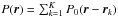 , leading to the MTF T(u) by means of the autocorrelation function of the aperture, in units of wavelength. The product T(u)Ô(u) gives the image transform Î(u), which is the common point after which the two simulations differ. Taking the inverse Fourier transform of Î(u) directly infers the (dirty) image I(α) that can be observed at the focus of a perfect turbulence-free stellar interferometer. The densified image I′(α) is obtained through the transformations described by Eqs. (5) and (6).
To simulate realistic images obtained by a diluted array of telescopes, it is necessary to have a sufficiently large number of pixels to correctly sample each individual telescope.
Numerically, this involves a sampling over of the Fourier plane. A simple way of achieving this is to use zero padding of the discrete image O(α). This facilitates the frequency translations described in Eq. (5), from Î(u) to in the diagram of Fig. 2.
While several parameters (number of telescopes, apertures sizes, and configuration) have a direct impact on the quality of the final image, it is unnecessary to optimize these parameters to check if a deconvolution technique can improve the hypertelescope image. Thus, any non-redundant configuration may be used for this demonstration. The greater the number and sizes of apertures, the greater the number of pixels in the images. Since we use iterative algorithms for the deconvolution, we limited the image size to 1024 × 1024 pixels for the deconvolution of images obtained in the FSD mode over a large number of iterations, or 2048 × 2048 for the comparison of images obtained with the FAD and FSD modes.
The number of telescopes is here K = 25, all apertures to be identical circular apertures of diameter D, set on a regular grid in x and y, with a minimal distance d = dm between them. In Fig. 3, we show the apertures positions in the configuration that we use (one among many possible). Making it non-redundant makes it possible to obtain the largest number of independently sampled spatial frequencies for this number or telescopes, and to recover images good enough for a visual interpretation. The figure is drawn in units of dm. The real array transmission P(r) can be obtained by substituting the elementary aperture P0(r) for the positions indicated in Fig. 3, and by giving to d a sufficiently large value. In the same figure, we also represented the ensemble of differences of positions ukl that appear in Eq. (4) and provide the Fizeau MTF T(u). This figure is drawn in units of dm/λ. Since the array is fully non-redundant, with K = 25, there are 601 regions of the Fourier plane associated with the array. In addition to the central region, for which all apertures contribute, there are K(K − 1) = 600 regions corresponding to every possible pair of apertures, all transmitted with the amplitude 1/K = 1/25. Half of these 600 regions correspond to symmetric positions. For arrays of 1024 × 1024 points, our simulation is made for dm = 7 units and D = 1.5, so that T0(u) is 3 × 3 points wide in the Fourier plane. For arrays of 2048 × 2048 points, our simulation is made for dm = 16 units and D = 3.5, so that T0(u) spreads over 7 × 7 points in the Fourier plane. Though the two cases are not entirely identical, they have strong similarities (7/3 ≈ 16/7 ≈ 2.3). Thus, a fair comparison can be made between the deconvolutions applied to the FSD and FAD modes (which are performed on arrays of 2048 × 2048 points) and the deconvolutions applied after rediluting the images taken in FSD mode (on arrays of 1024 × 1024 points).
Three examples of MTF, PSF, and images are given in Fig. 4 to illustrate the Fizeau case, the FSD case, and the FAD case. However, owing to the constraints in our numerical simulations, we cannot study a pure FAD case and have to approximate it: instead of considering a minimum distance of D between two apertures, we consider a minimum distance equal to 8/7 D. A more accurate approximation could be obtained for arrays composed of a greater number of points. For example, with arrays of 4096 × 4096 points, the minimum distance would be 14/13 D. Nevertheless, we believe that the difference between the true FAD mode and the approximation that we make has no consequences for the conclusion that we draw in the rest of the paper about the interests and limitations of the FAD and FSD modes.
Since the array rather regularly fills a low frequency square grid, the PSF shows a series of peaks that are also located on a square grid. Moreover, because there are gaps in the grid coverage of the MTF, a diffuse speckle-like pattern is present. The focal image given in Fig. 4 is the result of the convolution of the PSF with the object (here a low-resolution version of an image taken by NASA’s MODIS1). The Fizeau image appears as an ensemble of object replicas superimposed on a cloudy background. If the extent of the object is larger than the distance between peaks in the PSF, replicas of the Earth-like planet will overlap. A discussion of these effects is made in Aime (2008). A way to interpret these effects is to use the Shannon theorem, by reversing the usual two spaces, firstly dm playing the role of the sampling interval and secondly the extent of the astronomical object that of the usual frequency cutoff.
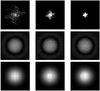 |
Fig. 4 Left: Fizeau mode. Middle: FSD mode. Right: pseudo-FAD mode. Top: autocorrelations. Center: PSF. Bottom: focal plane images. |
A few elements of the simulation of the hypertelescope image in the FAD and FSD cases are also given in the same Fig. 4. The operation of densification in the Fourier space is similar to that shown in Fig. 1. Since we now have 601 regions, it is no longer possible to represent the image with its full resolution as we did before, and the values of Î(u) and Î′(u) are clipped to black and white. In the simulation, the densification parameter γ is approximately equal to 7/3 ~ 2.3 (dm = 7 and to  ), which corresponds to the FSD case. Because of this shift to lower frequency structures, the resulting densified image I′(α) appears as a zoomed version of the Fizeau image, as described by Aime (2008).
2.3. Photodetected images
The procedure we use to simulate the photodetected images is based on the semi-classical theory of photodetection. Goodman (1985) assumes a classical propagation of the light down to the detector, using the Huygens-Fresnel theory of wave propagation, and the quantum part is introduced in the transformation of the energy that arrives at a pixel’s location into photoelectrons. Assuming that an integrated energy m arrives at a pixel, m being a real positive number measured in units of photon energy hν, the possible integer number of photoelectrons n can be simulated using a random draw that obeys the Poisson distribution of mean m, i.e. a law of the form P(n/m) = e − mmn/n ! .
From a practical point of view, we start from discrete representations of the deterministic images I(α) and I′(α). We associate the pixels of these images with the elements of a two-dimensional detector. In what follows, we work with simulated images of 1024 × 1024 pixels. We assume that in average an image is formed of a number N of photons. For each pixel, we then proceed to a random draw using a Poisson process of mean value the number of photons mij that changes from one pixel to an other.
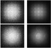 |
Fig. 5 Effect of the application of a pre-filter on photodetected images of Fig. 4 for ~1 million photons per image. Top: direct Fizeau images, bottom: FSD hypertelescope images, left: before and right: after application of the filter. |
In the example of Fig. 5, we have represented the photodetected Fizeau and FSD images of Fig. 4, for N = 106 photons. The mean number of photons per pixel is then ~0.95. The mij are real positive numbers smaller than a maximum of ~3.7, which are the same in the direct and densified images. There are no more photons per pixel in the densified image than in the direct image because of the zooming effect (pixels correspond to different angular units in the two images). If a de-zooming were applied, the number of photons per pixel in the densified image would increase as γ2, i.e. by a factor of about 5.4. The interest in the densification would be more obvious if γ could be larger, but this would also require an increase in the number of pixels in the images, thus an increase in computation time when applying the deconvolution algorithms. In the procedure we used, the final total number of photons in the images is not exactly N, but fluctuates around N with a standard deviation of  . The examples of photodetected images shown in Fig. 6 indeed correspond to photon numbers of 999 960 and 999 355. These numbers differ negligibly from N = 106 when a fair comparison between the two images is done.
These images appear to be very noisy. It is however easy to improve them using a simple linear filtering, which we now describe. We know that because the photodetection is a Poisson process, a white noise is superimposed on the image spectrum. Since we know the domain of frequencies transmitted by the array of telescopes, we can suppress this noise in the region of the spectrum where no signal is expected. Thus, for the Fizeau image, we can multiply the spectrum by the indicator function of the MTF T(u), a function equal to 1 for T(u) ≠ 0 and 0 elsewhere. We denote this function Z(u), and can compute it as sign( | T(u) | ). The filtered direct image is ![Mathematical equation: \hbox{$I_{pZ}(\boldsymbol \alpha)=|\mathcal{F}^{-1}[Z(\boldsymbol u) \hat{I_p}(\boldsymbol u)] |$}](/articles/aa/full_html/2012/07/aa17554-11/aa17554-11-eq98.png) . It is necessary to take the absolute value (or alternatively the positive value) of the final image to get rid of small negative values, which are artifacts that appear when taking the Fourier transform of the filtered image. A similar operation can be applied to the densified image. The results are shown in Fig. 5. This filtering produces an apparently great improvement in the direct noisy image. In term of the application of a deconvolution algorithm, the images after deconvolution are indeed quite insensitive to this pre-filtering.
. It is necessary to take the absolute value (or alternatively the positive value) of the final image to get rid of small negative values, which are artifacts that appear when taking the Fourier transform of the filtered image. A similar operation can be applied to the densified image. The results are shown in Fig. 5. This filtering produces an apparently great improvement in the direct noisy image. In term of the application of a deconvolution algorithm, the images after deconvolution are indeed quite insensitive to this pre-filtering.
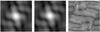 |
Fig. 6 Left and middle: two point-like sources observed at different positions on the sky by the densified array. Right: absolute difference of the two previous images. |
3. Image enhancement using the deconvolution algorithms
3.1. Brief presentation of the image space reconstruction (ISRA) and Richardson-Lucy algorithms
Two classical types of noise can be considered in astronomy: Gaussian and Poisson noise. In the present analysis, we consider two algorithms that similarly minimize the negative log-likelihood of these two noises.
For an additive, zero mean, Gaussian white noise, the deconvolution can be performed by means of the Image Space Reconstruction Algorithm (ISRA) (Daube-Witherspoon & Muehllehner 1986). The aim of this iterative multiplicative algorithm is to minimize the negative log likelihood of data corrupted by a Gaussian noise process, that is the Euclidean distance between the noisy data and the convolutive model, subject to the non-negativity constraint of the successive estimates. The convergence of this algorithm was analyzed by De Pierro (1987) and in its relaxed form by Lantéri et al. (2002).
The classical multiplicative form of ISRA can be written as 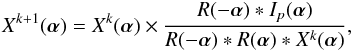 (7)where Xk(α) is the estimate at the iteration k for the object O(α) we seek to recover and R(α) the PSF.
For a Poisson noise process, the deconvolution is generally performed by means of the iterative algorithm proposed by Lucy (1974) and Richardson (1972). This algorithm belongs to the general approach of the Expectation Maximization (EM) algorithm (Dempster et al. 1977; Rubin 1977). It has been shown that this algorithm maximizes the likelihood for data corrupted by a Poisson noise process, subject to a non-negativity constraint of the estimates. In an equivalent way, it can be considered as an algorithm that minimizes the negative log-likelihood that is the Kullback-Leibler divergence between the noisy data and the convolutive model, subject to a non-negativity constraint. The classical multiplicative form of RLA can be written as  (8)For both algorithms, the iterative process generally starts with an initial estimate X0(α), whose value is a constant that equals the mean of Ip(α).
The effect of these algorithms is well-known when the PSF R(α) corresponds to a low-pass filter. Roughly speaking, during the iterative process, the low spatial frequencies are reconstructed first and the higher frequencies appear progressively when the iteration number increases. The main drawback of the iterative algorithm, as well as all other non-regularized deconvolution algorithms, is that the deconvolution problem is an ill-posed problem (Bertero & Boccacci 1998), and as a consequence the reconstructed image becomes very noisy when the iteration number becomes too large. To avoid this problem, the classical ways of solving this problem are either to regularize explicitly (Lantéri et al. 2002) the problem by introducing at some level a smoothness penalty, or to stop the iterative process before noise amplification that corresponds to a smoothing operation.
We see in the simulation that the effects of both RLA and ISRA on the interferometric and hypertelescope images is more complex, and that the filling of spatial frequencies spreads from areas transmitted by the diluted array.
3.2. Deconvolution applied to the densified image
We intend to test the deconvolution procedure by applying it to densified images, independent of the degree of densification. In practice, we give illustrations for rates corresponding to the FSD and pseudo-FAD modes.
The exact object-image relationship for an hypertelescope is described by a Fredholm integral for a non-separable space-variant PSF. According to Andrews & Hunt (1977), this involves the manipulation of a N2 × N2 matrix for a N × N image, e.g. a one million square matrix for an image of 1000 × 1000 pixels. This exceeds the possibilities of current computers.
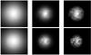 |
Fig. 7 Deconvolution of densified noiseless images. From left to right: result of RLA for k = 10,100,1000. Top: FAD. Bottom: FSD. |
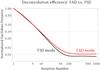 |
Fig. 8 Efficiency of the RLA deconvolution when operating in the FAD and FSD modes (respectively red and black solid lines). |
As claimed by Labeyrie (2007), for an object of small angular extent, the hypertelescope performs a pseudo-convolution, and we can try to apply a direct deconvolution technique assuming a space-invariant PSF. We assimilate this PSF to the response of the densified array for the center of the field. We assume that the PSF R′(α) is simply the Fourier transform squared of the densified MTF T′(u). The images of two point-like sources located at two different positions are indeed very similar. An example of two such responses, is shown in Fig. 6. The differences are indeed very small, leading to a mean normalized Euclidean distance of 0.35% between numerous pairs of sources. These slight differences seems to justify the direct use of a deconvolution technique.
Figure 7 shows the output of the RLA X′k(α) at iterations k = 10,100,and1000, for the FSD and FAD modes. The results are disappointing, especially for the FAD mode, but this is not unexpected. Results obtained with ISRA are very similar but not given here for the sake of conciseness.
Figure 8 details the evolution of the normalized Euclidean distance between the deconvolved images resulting from the two densification modes (FSD and FAD) and the true object. As can be seen in this figure, both distances decrease sharply with the iteration number until they reach a minimum value. In both cases, this value is reached for k ~ 100. They are however different, and images obtained in the FSD mode are slightly closer to the original image than images obtained in the FAD mode. This is explained by the autocorrelation peaks being partially mixed, making it impossible for the deconvolution algorithm to distinguish the information they contain.
None of the results are truly satisfactory.
Since the application of the deconvolution algorithms cannot provide good results in the noiseless case, it is unsurprising that similarly poor results are obtained for the photodetected image  . An example of
  for k = 100 and k = 590 is shown in Fig. 9. We can deduce from this study that the raw deconvolution of densified data never gives satisfactory results, regardless of the degree of densification.
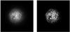 |
Fig. 9 Result of the application of RLA to |
3.3. MTF redilution: recovering the true convolution relationship
One may conclude that the problems encountered during the deconvolution of a raw densified image are due to the lack of a true convolution relationship. There is indeed a way to try to recover that relation.
We assume that a telescope operates in a densified mode and has produced the densified image I′(α). It is possible to recover the Fizeau image I(α) by inverting, using a numerical post-process, the operation of densification. The technique, which consists of a redilution, was previously described in Tallon & Tallon-Bosc (1992) and in a different context by Guyon & Roddier (2002) for coronagraphic applications. We note that this operation is possible only for γ values smaller than that corresponding to FSD mode. For larger values, spectral overlapping occurs.
3.3.1. Noiseless images
We first consider the case of the noiseless image. There is here no specific reason to choose ISRA over RLA, or conversely, RLA over ISRA, since these algorithms have been developed for specific types of noise. To recover the Fizeau image I(α), we start by computing the Fourier transform Î′(u) of I′(α). The frequency domains around are then shifted back to their original positions ukl. We therefore obtain a quantity equal to Î(u), and the Fizeau image I(α) can be simply obtained by an inverse Fourier transform. The relation of convolution is now recovered, the PSF being that of the Fizeau array. We note that this step is performed in a post-process, and without any signal deterioration.
We run the deconvolution algorithm up to the iteration k = 50 000. After a few hundred iterations, the replicas in the original image disappear and only a single central image of the Earth-like object remains. In these first steps, the deconvolution gathers the replicas by means of a computation process. In this view, the deconvolution process achieves numerically an operation analogous to that performed by the hypertelescopes with an optical device.
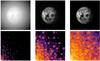 |
Fig. 10 Deconvolution of rediluted noiseless images. Top: from left to right, result of RLA on the re-diluted images for k = 10,1000, and 10 000. Bottom: corresponding modulus in the Fourier plane. Only a limited part of the first quadrant of the Fourier plane is shown. |
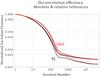 |
Fig. 11 Euclidean distance computed between the result of the deconvolution and the original object (solid lines), or its image as seen by the meta telescope (dashed lines, see Fig. 12). Black: RLA. Red: ISRA. |
The way in which the deconvolution algorithms delete replicas can be well-understood in the Fourier plane (Fig. 10, bottom figures). The algorithms RLA and ISRA are non-linear and extend the frequency spectral range of the image (Lantéri et al. 1999). For the diluted array, the coverage of the angular frequencies preferentially grows from known spectral regions. As the number of iterations increases, these algorithms spread energy into the missing zones of the spectrum, thus populating the gaps between the known frequency regions. This can be considered as an inpainting of the Fourier plane. Once the gaps are filled, there is no more reasons for replicas to appear in the reconstructed image.
The deconvolution can then continue, making it possible to recover yet more intricate details of the astronomical object. This requires a much larger number of iterations (a few thousands), as it can be seen in Fig. 10, which gives the results restricted to the central part of the image (top line), and its counterpart in a limited area of the first quadrant of the Fourier plane. In Fig. 11, we have indicated by solid lines the evolution of the Euclidean distance between the original image and the result of both deconvolution processes from k = 1 to k = 50 000. It can be seen that, as a result for the noiseless data, the quality of the reconstructed image increases monotonically with the number of iterations. After k = 5000 or so, the image improvement is very slow. As expected, the behavior of both algorithms is very similar, and they reach the same values. When comparing these curves with those obtained for the deconvolution of the densified image (Fig. 8), we can see the improvement in the results. It is excellent, especially when compared to what can be obtained with the raw meta telescope image shown in Fig. 12.
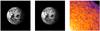 |
Fig. 12 Images of the original object (left) and as seen by the meta telescope (center). The modulus in the Fourier plane of the latter is also displayed (right). |
Although the results of RLA and ISRA must fundamentally be compared to the original image O(α), they can be compared to the image Im(α) that the meta telescope would give. The result is shown in Fig. 11 (dashed lines). For comparison, the distance to the original image is also given (continuous lines). We can observe that regardless of the reference image, the two algorithms converge toward the same value. The distance is however smaller for the reference image Im(α). As a matter of fact, in the absence of photodetection noise, the image obtained for k = 50 000 compares favorably with the direct image obtained with the meta telescope, independently of the algorithm used.
3.3.2. Noisy images
We now consider the case of noisy data. The operation of image redilution for noisy data is more tricky. Whatever the origin of the noise, the image obtained after redilution is corrupted by a noise whose statistical properties are unknown. The redilution indeed changes the properties of the noise. There is then no strong reason to prefer one algorithm over the other. Fortunately, we are able to show that both algorithms lead to almost similar results.
As already discussed for the application of the filter Z(u), the image spectrum is contaminated by a noise that spreads over the whole frequency plane, particularly in areas where there is no expected signal. We cannot handle the redilution of the noise spectrum per se. What we can do is to set to zero the values of that are in the region where no signal is expected, i.e. apply a filter such as Z(u). We note that this does not suppress the noise, but limits its influence to the regions where the signal is expected. The rediluted and pre-filtered image shown in Fig. 13 (left), appears to be very similar to the pre-filtered Fizeau image of Fig. 5. The difference between them, shown in absolute value in the right image of Fig. 13 is compatible with statistical fluctuations.
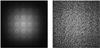 |
Fig. 13 Left: FSD hypertelescope image after MTF redilution. Right: absolute difference between this image and the interferometric image shown in Fig. 5. Differences are due to the statistical origin of the photodetection process. |
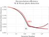 |
Fig. 14 Efficiency of the deconvolution algorithms with and without a photon noise (represented in dashed and solid lines, respectively). The color code is the same as in Fig. 11. |
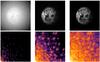 |
Fig. 15 Image restoration in the presence of photodetection noise: Top: from left to right, result of RLA on the re-diluted images for k = 10, 1000, and 10 000. Bottom: corresponding modulus in the Fourier plane. |
The effect of the algorithm on this noisy image is shown by the Euclidean distance drawn in Fig. 14 (dashed lines). In the same figure, we also show the equivalent curves for the noiseless case, which have been previously given in Fig. 11. It can be seen that the curves for the noisy case are very similar for both algorithms. Moreover, the reconstruction error increases with the iteration number, after having passed through a minimum. This is a classical behavior for non-regularized deconvolution problems. To prevent this phenomena, we can either stop the iterations before noise amplification or use an explicitly regularized algorithm. Here, as already indicated, we just stopped the iterations k. In our example, there is a flat minimum around k = 2000, as shown by the Euclidean distance drawn in Fig. 14. There are indeed very few differences for a broad range of k values, between 600 to 10 000 or so. An example of the reconstructed images for several values k is shown in Fig. 15. The reconstructed image spectrum presents the same behavior as for the noiseless data, i.e. a filling of spatial frequencies that develops from known regions of the spectrum, i.e. corresponding to an inpainting of the Fourier plane. Noise amplification arises for k values larger than a few thousands, as illustrated by the result for k = 10 000.
4. Discussion and conclusion
In this paper, we have focused on improving the snapshot image given by an hypertelescope using deconvolution techniques.
We have considered two types of hypertelescopes. The first one consists of a complete densification of the pupils which is denoted here by FAD and originally proposed by Labeyrie (2007). The other one corresponds to a complete densification of only the MTF, referred to herein as FSD. The application of a direct deconvolution of images obtained by a hypertelescope, whether in the case FSD or FAD did not give good results. This was an unsurprising result. Our interpretation is that because the hypertelescope mode is no longer represented by a convolution relationship, there is no reason to assume that a simple deconvolution can invert the Fredholm relation for an angular-dependent PSF. Because the variation in the impulse response across the field is very small, Labeyrie’s suggestion to replace the Fredholm relation with a simple convolution had to be tested, though the result is unfortunately unsatisfactory.
We have presented in this paper a practical way of improving an hypertelescope image. The procedure involves two steps, a first of which numerically re-dilutes the hypertelescope image to artificially retrieve a Fizeau image. We emphasize that this cannot be done for the FAD mode of operation (because the complex amplitudes from the different apertures are entangled), and that the FSD mode is the maximum densification for which it is possible to apply a redilution (or de-densification) without difficulty. In the second step, the application of a deconvolution to these images is then legitimate and gives excellent results. We discuss the problems that occur when photon noise is taken into account. This study thus leads to a practical result of interest to researchers wishing to use a hyperspectral technique. We advise
them not to use a densification stronger than FSD if they wish to further improve the quality of the image by deconvolution. This result is not unexpected, but useful to recall, especially when considering all the experimental efforts underway to develop hypertelescopes in the FAD mode.
References
- Aime, C. 2008, A&A, 483, 361 [NASA ADS] [CrossRef] [EDP Sciences] [Google Scholar]
- Andrews, H. C., & Hunt, B. R. 1977, Digital image restoration (Prentice Hall) [Google Scholar]
- Bertero, M., & Boccacci, P. 1998, Introduction to inverse problems in imaging (IoP Publishing) [Google Scholar]
- Daube-Witherspoon, M. E., & Muehllehner, G. 1986, IEEE Trans. Med. Imgng., 61 [Google Scholar]
- De Pierro, A. R. 1987, IEEE Trans. Med. Imgng., 174 [Google Scholar]
- Dempster, A. D., Laird, N. M., & Rubin, D. B. 1977, J. Roy. Stat. Soc., 1 [Google Scholar]
- Goodman, J. W. 1985, Stat. Opt. (New York: Wiley-Interscience) [Google Scholar]
- Guyon, O., & Roddier, F. 2002, A&A, 391, 379 [NASA ADS] [CrossRef] [EDP Sciences] [Google Scholar]
- Kopilovich, L. E., & Sodin, L. G. 2001, Multielement system design in astronomy and radio science, Astrophysics and Space Science Library (Dordrecht: Kluwer Academic Publishers), 268 [Google Scholar]
- Labeyrie, A. 1975, ApJ, 196, L71 [NASA ADS] [CrossRef] [Google Scholar]
- Labeyrie, A. 1996, A&AS, 118, 517 [NASA ADS] [CrossRef] [EDP Sciences] [Google Scholar]
- Labeyrie, A. 2007, Compt. Rendus Phys., 8, 426 [Google Scholar]
- Lantéri, H., Soummer, R., & Aime, C. 1999, A&AS, 140, 235 [NASA ADS] [CrossRef] [EDP Sciences] [Google Scholar]
- Lantéri, H., Roche, M., & Aime, C. 2002, Inv. Probl., 18, 1397 [CrossRef] [Google Scholar]
- Lardière, O., Martinache, F., & Patru, F. 2007, MNRAS, 375, 977 [NASA ADS] [CrossRef] [Google Scholar]
- Lucy, L. B. 1974, AJ, 79, 745 [NASA ADS] [CrossRef] [Google Scholar]
- Michelson, A. A. 1920, ApJ, 51, 257 [NASA ADS] [CrossRef] [Google Scholar]
- Michelson, A. A., & Pease, F. G. 1921, ApJ, 53, 249 [NASA ADS] [CrossRef] [Google Scholar]
- Mourard, D., Tallon-Bosc, I., Blazit, A., et al. 1994, A&A, 283, 705 [NASA ADS] [Google Scholar]
- Mourard, D., Clausse, J. M., Marcotto, A., et al. 2009, A&A, 508, 1073 [NASA ADS] [CrossRef] [EDP Sciences] [Google Scholar]
- Ohnaka, K., Weigelt, G., Millour, F., et al. 2011, A&A, 529, A163 [NASA ADS] [CrossRef] [EDP Sciences] [Google Scholar]
- Patru, F., Mourard, D., Clausse, J.-M., et al. 2008, A&A, 477, 345 [NASA ADS] [CrossRef] [EDP Sciences] [Google Scholar]
- Patru, F., Tarmoul, N., Mourard, D., & Lardière, O. 2009, MNRAS, 395, 2363 [NASA ADS] [CrossRef] [Google Scholar]
- Richardson, W. H. 1972, J. Opt. Soc. Am. (1917-1983), 62, 55 [Google Scholar]
- Rubin, A. P. D. N. M. L. D. B. 1977, J. Roy. Stat. Soc. Ser. B (Methodological), 39, 1 [Google Scholar]
- Tallon, M., & Tallon-Bosc, I. 1992, A&A, 253, 641 [NASA ADS] [Google Scholar]
- ten Brummelaar, T. A., McAlister, H. A., Ridgway, S. T., et al. 2005, ApJ, 628, 453 [NASA ADS] [CrossRef] [Google Scholar]
- Thiebaut, E., & Giovannelli, J.-F. 2010, IEEE Signal Proc. Mag., 27, 97 [NASA ADS] [CrossRef] [Google Scholar]
All Figures
|
Fig. 1 Top: from left to right: a monolithic giant aperture (the so-called meta-telescope), a diluted array of four telescopes in Fizeau mode and in the two hypertelescope modes FSD and FAD. Bottom: phase of the image transform for the test object, which clearly illustrates it visible the aliasing effect in the FAD mode. This aliasing makes it impossible to recover the Fizeau spectrum in the FAD mode, while the inverse operation remains possible in the FSD mode. |
| In the text | |
|
Fig. 2 Block-diagram of the numerical simulation giving the interferometric and hypertelescope images at high light level (I(α) and I′(α)) and in photodetection mode (Ip(α) and |
| In the text | |
|
Fig. 3 Example of positions for a configuration of 25 point-like non-redundant apertures (left), with its corresponding autocorrelation function (right). |
| In the text | |
|
Fig. 4 Left: Fizeau mode. Middle: FSD mode. Right: pseudo-FAD mode. Top: autocorrelations. Center: PSF. Bottom: focal plane images. |
| In the text | |
|
Fig. 5 Effect of the application of a pre-filter on photodetected images of Fig. 4 for ~1 million photons per image. Top: direct Fizeau images, bottom: FSD hypertelescope images, left: before and right: after application of the filter. |
| In the text | |
|
Fig. 6 Left and middle: two point-like sources observed at different positions on the sky by the densified array. Right: absolute difference of the two previous images. |
| In the text | |
|
Fig. 7 Deconvolution of densified noiseless images. From left to right: result of RLA for k = 10,100,1000. Top: FAD. Bottom: FSD. |
| In the text | |
|
Fig. 8 Efficiency of the RLA deconvolution when operating in the FAD and FSD modes (respectively red and black solid lines). |
| In the text | |
|
Fig. 9 Result of the application of RLA to |
| In the text | |
|
Fig. 10 Deconvolution of rediluted noiseless images. Top: from left to right, result of RLA on the re-diluted images for k = 10,1000, and 10 000. Bottom: corresponding modulus in the Fourier plane. Only a limited part of the first quadrant of the Fourier plane is shown. |
| In the text | |
|
Fig. 11 Euclidean distance computed between the result of the deconvolution and the original object (solid lines), or its image as seen by the meta telescope (dashed lines, see Fig. 12). Black: RLA. Red: ISRA. |
| In the text | |
|
Fig. 12 Images of the original object (left) and as seen by the meta telescope (center). The modulus in the Fourier plane of the latter is also displayed (right). |
| In the text | |
|
Fig. 13 Left: FSD hypertelescope image after MTF redilution. Right: absolute difference between this image and the interferometric image shown in Fig. 5. Differences are due to the statistical origin of the photodetection process. |
| In the text | |
|
Fig. 14 Efficiency of the deconvolution algorithms with and without a photon noise (represented in dashed and solid lines, respectively). The color code is the same as in Fig. 11. |
| In the text | |
|
Fig. 15 Image restoration in the presence of photodetection noise: Top: from left to right, result of RLA on the re-diluted images for k = 10, 1000, and 10 000. Bottom: corresponding modulus in the Fourier plane. |
| In the text | |
Current usage metrics show cumulative count of Article Views (full-text article views including HTML views, PDF and ePub downloads, according to the available data) and Abstracts Views on Vision4Press platform.
Data correspond to usage on the plateform after 2015. The current usage metrics is available 48-96 hours after online publication and is updated daily on week days.
Initial download of the metrics may take a while.