| Issue |
A&A
Volume 535, November 2011
|
|
|---|---|---|
| Article Number | A11 | |
| Number of page(s) | 7 | |
| Section | Interstellar and circumstellar matter | |
| DOI | https://doi.org/10.1051/0004-6361/201117390 | |
| Published online | 25 October 2011 | |
The high resolution X-ray spectrum of SNR 0506-68 using XMM-Newton
1
Astronomical Institute, University of Utrecht, Postbus 80000, 3508 TA Utrecht, The Netherlands
e-mail: s.broersen@astro-uu.nl
2
SRON, Netherlands Institute for Space Research, Sorbonnelaan 2, 3584 CA Utrecht, The Netherlands
3
Harvard-Smithsonian Center for Astrophysics, 60 Garden Street, Cambridge, MA 02138, USA
Received: 31 May 2011
Accepted: 30 August 2011
Aims. We study the supernova remnant 0506-68 in order to obtain detailed information about, among other things, the ionisation state and age of the ionised plasma.
Methods. Using the Reflection Grating Spectrometer (RGS) onboard the XMM-Newton satellite we are able to take detailed spectra of the remnant. In addition, we use the MOS data to obtain spectral information at higher energies.
Results. The spectrum shows signs of recombination and we derive the conditions for which the remnant and SNR in general are able to cool rapidly enough to become over-ionised. The elemental abundances found are mostly in agreement with the mean LMC abundances. Our models and calculations favour the lower age estimate mentioned in the literature of ~4000 year.
Key words: ISM: supernova remnants / supernovae: general
© ESO, 2011
1. Introduction
Supernova remnants (SNRs) hold important information about the nucleosynthesis and energy of the supernova explosion, its circumstellar matter (CSM) evolution and the physics of the ionised plasmas. The Large Magellanic Cloud (LMC) is particularly well suited for the study of SNRs, since the absorption column to the LMC is low and it is relatively close (50 kpc). Moreover, studying SNRs in the LMC has the advantage that the distance is known quite precisely, which is convenient for luminosity and length scale calculations.
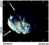 |
Fig. 1 A smoothed Chandra RGB image of the SNR 0506-68. The arrows denote the direction of the RGS dispersion directions. The RGS field of view covers the remnant completely. Red corresponds to O vii (0.53−0.61 keV), green to Fe l (0.79 − 0.89 keV) and blue to Mg xi (1.25 − 1.41 keV). The arrows denote the dispersion axis orientation of the 2000 (upper arrow) and the 2002 (lower arrow) observations. |
SNR 0506-68 (also known as N23) is a small (R ~ 10 pc, see Fig. 1) remnant located fairly centrally in the LMC. The X-ray emission of the remnant is characterised by a filamentary structure with some bright spots. There is a gradient in brightness running from southeast to northwest. The remnant has been studied by Hughes et al. (2006) with the Chandra telescope. Both Hughes et al. (2006) and Hayato et al. (2006) report the presence of a compact object and conclude that the SNR is a result of a core-collapse supernova explosion (SNe). They find that the X-ray emission comes largely from the swept-up interstellar medium and estimate the age of the remnant to be ~4600 yr. Recently, Someya et al. (2010) used the XIS instrument onboard the Suzaku telescope to obtain a more detailed spectrum of SNR 0506-68. They note the presence of a cool (~0.2 keV) temperature component in addition to a hot (~0.6 keV) component in the plasma, and a high ionisation parameter net (~1013 cm-3 s). From a Sedov analysis they conclude that the age of the remnant, based on the cool component, may be as high as ~8000 yr, but that it may have entered the radiative phase of its evolution. If the age is indeed as high as 8000 yr that would mean that the size of the remnant is quite small for its age, suggesting that the explosion took place in a high density region of the LMC.
It has long been recognized that when a gas is suddenly heated in a shock it is under-ionised, and requires a density-weighted time scale net ~ 1012 cm-3 s to approach equilibrium (Smith & Hughes 2010). Recently, however, two groups have reported evidence for over-ionised plasma in the SNRs W49B and IC 443 (Yamaguchi et al. 2009; Ozawa et al. 2009; Miceli et al. 2010). In this paper we aim to obtain detailed understanding about the ionised plasma of SNR 0506-68 using the spectral diagnostic capacity of the RGS (Reflection Grating Spectrometer) instrument (den Herder et al. 2001). High resolution spectra of SNRs, obtained with grating spectrometers such as the RGS, hold detailed information about the ionised plasma. The spectral resolution of the RGS is large enough to resolve, among others, the OVII He-α triplet at ~22 Å and the Fe xvii line complex around 15 − 17 Å, provided the source has a small angular extent. The ratios of different emission lines in these elements provide interesting plasma diagnostics (e.g.: Porquet et al. 2010).
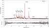 |
Fig. 2 The total 2001 RGS1 and RGS2 spectrum of SNR 0506-68 in the range 5 − 35 Å. The best fit two-component NEI model (see text) is plotted in red. |
2. Data
We used the data obtained by the XXM-Newton satellite on July 6, 2000 (obs ID 0111130101) and July 10, 2002 (obs ID 011130701). The exposure times of the observations are 18.1 and 19.7 ks. For our spectral study, we made use of the RGS and EPIC MOS (Turner et al. 2001) data. Although the EPIC pn camera has a higher sensitivity, the MOS cameras have a higher spectral resolution, which is important for comparison with the RGS data. All MOS observations were performed in full frame mode with the medium filter in place.
The 2000 RGS observation was taken with the dispersion direction oriented 27° counterclockwise from the celestial north, while the 2002 observation was rotated 90° with respect to this observation, at a dispersion direction orientation of 117° (see Fig. 1). This resulted in different line profiles which need separate responses, as the 2002 observation has a higher effective resolution than the 2000 one. The RGS data were corrected for periods of high background flaring by creating good time intervals based on the count rate in CCD number 9 of the instrument. This CCD is closest to the optical axis of the telescope and therefore affected most by background flaring. The second order spectra have a higher resolution, but are of lower statistical quality. Since they provide no additional information they are not presented here.
The RGS is a slitless spectrometer. When using this kind of instruments, the lines in the spectra get smeared out as a result of the extent of the source. Although the angular size of SNRs observed in the LMC is modest, this smearing is still present. We corrected for this using the heasoft program rgsrmfsmooth (A. Rasmussen). This program calculates a brightness profile, based on an image, in the direction of the RGS dispersion axis. It then uses this profile to adjust the response matrix to correct for the line smearing. In our analysis a Chandra image was used to create the profile, to obtain maximum precision in the correction.
The spectra were analysed using the SRON SPEX package (Kaastra et al. 1996). Before the spectra were fit, we performed the SPEX optimal binning. This bins the data into optimal bins, making use of the statistics of the source as well as the instrumental resolution.
All standard RGS and MOS reduction tasks were done using XMM SAS version 10.0.0.
3. Results
3.1. Overall spectra
The total RGS spectrum of SNR 0506-68 is shown in Fig. 2 and the MOS spectrum is shown in Fig. 3. As is clear from Fig. 2, the spectrum is dominated by emission lines of highly ionised O, Fe, Ne, N and C . The oxygen emission is particularly present with the notable O vii line triplet at ~22 Å and the O viii lines at ~19 and ~16 Å. The fact that both Ne and C are present suggests that there exist both a cool and hot component in the local plasma. Thus, like Someya et al. (2010), the spectra were fit using two non-ionisation equilibrium (NEI) models. This model attempts to fit the data with two values of the parameters emission measure ne nH VX, electron temperature Te and ionisation age net. We used the standard SPEX absorption model to produce the hydrogen column NH to the remnant. Before fitting with the RGS, we first obtained the high T continuum slope by fitting the MOS data. When fitting the RGS data, the abundances were first fixed at the LMC/ISM abundances found by Hughes et al. (1998), and the ionisation parameters of the two NEI components were coupled. When the different temperatures of the models had converged, the ionisation parameters as well as some of the abundances were released to obtain a better fit.
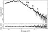 |
Fig. 3 Plot of the MOS 1 and MOS 2 data of 2002. The model seems to fit the data well. |
RGS data C-stat/d.o.f. of the tried models for the different observations.
For the RGS data, models with different ionisation timescales net and temperatures T give more or less comparable fits to the data. The models that were investigated can roughly be divided into four categories which are listed in Table 1. The model listed at the bottom row of the table (model D) consists of two NEI components which are in ionisation equilibrium, i.e.: net ≥ 1012 cm-3 s. This model is comparable to the best fit model found by Someya et al. (2010). A lower C-statistic was found for a two component NEI model, in which one of the components had a somewhat lower ionisation timescale (model C). This indicates that at least part of the remnant’s plasma is out of ionisation equilibrium. The two best-fit models of Table 1 are a two component NEI model, in which both components have a low net (model A) and a cooling model (model B, explained below). Because the difference in C-statistic between these models is very minor, considering the amount of degrees of freedom, we listed the parameters of both the models in Table 2. The ionisation parameters of model A and B are comparable to those found by Hughes et al. (2006).
The best fit model of the 2002 RGS spectrum, the cooling model (model B), deserves special attention. This is a model in which one of the NEI components is inverted, i.e.: the initial temperature of this component is higher than the final temperature. This cooling model, with an initial temperature of 3.0 keV, reproduces especially the O vii resonance to forbidden line ratio better than a non-cooling two temperature NEI model. Furthermore it produces radiative continua in the higher energy parts of the spectrum, which become important in the MOS spectra. Physically, the cooling model corresponds to a plasma for which the cooling rate exceeds the recombination rate, which can cause overionisation. As mentioned in the introduction, rapidly cooling plasmas have been observed before in, among others, the mixed morphology remnants IC 443 and W49B. The fact that the overionisation model works well for SNR 0506-68 could mean that overionisation is not limited to mature SNRs of the mixed morphology class alone.
The MOS spectra were also fit with different combinations of net and T, similar to the RGS data. Again, model A and model B gave the best fit to the data. In contrast to the RGS data, however, the difference in best fit C-statistic between model A and B is significant for the MOS data, namely 100σ. When comparing the fits of model A and B, it is not immediately clear where the difference of 100σ in C-stat comes from. Distinct radiative recombination edges, as have been observed in e.g. W49B, are not clearly visible in our spectrum. Nevertheless, a more detailed inspection reveals statistically significant differences. Figure 4 shows the model fits in the energy range 0.8 − 1.8 keV. The dashed red line shows the best fit model, model B, while the black line shows model A. The bottom part of the figure shows the residuals of the data with model A, with the difference between model B and A plotted as a dashed red line. This shows that model B follows the overall shape of the data better than model A. The presence of the Fe XVII recombination continuum at 1.26 keV, for example, improves the fit in the 1.2−1.3 keV range by lowering the C-stat by ~9σ.
As said, the abundances were coupled between the different model components. However, some parameters were decoupled to check if there were significant differences between the hot and cool component. The only significant difference occurred when the Fe abundances were decoupled. In all cases this lead to a significant improvement of the fit (the C-stat/d.o.f. decreased to 4144/2686 for our best fit model). The Fe abundance of the low temperature component jumped to values of five times solar in case of the RGS data, while the high temperature Fe abundance decreased to ~0.1 solar. In addition, the temperature of the lower T component decreased to a value of ~0.14 keV. It is possible that there is some cool Fe present in the SNR, as this has been found before in mature SNRs (e.g. Uchida et al. 2009). However, at a temperature of 0.14 keV the iron emission increases considerably when the temperature is raised by even a relatively small amount (~0.1 keV). It is possible that the Fe emission requires a higher temperature than other elements or that there are small temperature gradients present, and that the model compensates for this by increasing the Fe abundance. Since we considered a five times solar abundance of Fe non-physical in SNR 0506-68, we kept the abundances between the two model components fixed. The RGS is less sensitive at higher energies, so the MOS data were used to constrain the abundances of Mg, Si and S.
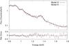 |
Fig. 4 A plot of the mos 2 data with model A and model B in the range 0.8 − 1.8 keV. The bottom part of the figure shows the relative error between model A and the data, while the dashed red line shows model B – model A. It is clear that model B follows the overall shape of the data better than model A. For example, model A shows a residual at ~1.25 keV, whereas model B improves the fit of this region due to the Fe xvii recombination edge at 1.26 keV. |
Best fit parameters for the 2 NEI and the cooling model.
3.2. Detailed line spectroscopy
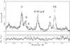 |
Fig. 5 The 2002 RGS1 and RGS2 spectrum of SNR 0506-68 in the range 14−18 Å. The best fit two-component NEI model (see text) is plotted in solid black. The model has trouble fitting the 15 and 17 Å Fe xvii as well as the O viii Ly β/Ly α line ratio. |
As shown above, model B, i.e. a cooling plasma, gives a good fit to our data. If the plasma is indeed rapidly cooling, there could be some other spectral indications. Below we will investigate several known plasma diagnostics to obtain detailed information about the spectrum.
An important diagnostic is the ratio of the different lines of the O vii line triplet. In the 2002 spectrum, the forbidden line at 22.08 Å is underestimated by the non-cooling model, while the resonance line at 21.6 Å is overestimated. As mentioned above, this line triplet was best reproduced by manually tweaking an NEI model to mimic a recombining plasma. Recombination preferentially populates the triplet levels that feed the forbidden line, while the resonance line is populated mainly by collisional excitation. As such, an enhanced forbidden line suggests the presence of enhanced recombination in the plasma. This will be discussed in more detail in paragraph 3.3.
Line fluxes of a number of emission lines calculated with and without hydrogen absorption.
All tested models have trouble fitting the Fe xvii 15 − 17 Å line ratio (see Fig. 5). These lines are formed by the transitions from the 3d and 3s levels of the Ne-like ion to the ground state. We used the same labeling of the lines that was used by Gillaspy et al. (2011). The fact that the 17 Å line blend is stronger than the 15 Å line can be another sign of enhanced recombination (Liedahl et al. 1990). To obtain the Fe xvii line ratios, the best fit overall model was used, while the contribution to the emission by Fe xvii lines was excluded from this model; this ensures that contributions from, e.g., higher lines of the O VIII Ly series are taken into account. The Fe xvii line complex in the range of 14 − 18 Å was then fit with five Gaussians, with a fixed NH of 1.14 × 1021 cm-2. The observed line strengths are listed in Table 3. We can compare our Fe xvii line ratios with recent laboratory measurements to obtain more information about the plasma. Gillaspy et al. (2011) measure the 3s/C and C/D ratios at different electron beam temperatures, where 3s = F+G+H. Our observed 3s/C ratio of 2.45 ± 0.2 and C/D ratio of 1.46 ± 0.13 both correspond to an electron beam temperature of ~0.85 keV, which is near the collisional excitation threshold. The observed line ratios show no indication of a high 3s/3d ratio indicative of recombination.
At 16 Å, the O viii Ly β line is underestimated by the model. By fitting the 15 − 20 Å region with an absorbed continuum and Gaussians, a Ly β/Ly α ratio of 0.13 ± 0.01 is obtained. This value is in agreement with CIE values found for this ratio at T ≃ 4 − 5 × 10⁶ K (Smith et al. 2001).
C vi at 33.7 Å also has a strong presence and is detected at a 9σ level. Because it is such a strong line, and it is affected heavily by absorption, it can be used to constrain the absorption column to the remnant. This was done by making a contour plot (Fig. 6) of the NH and the C abundance after a good fit was obtained. This resulted in an NH of 1.14 × 1021 cm-2, which was used in all our models. Note that in our model the C vi originates from the coolest component only (kT = 0.15−0.20 keV). At these temperatures C is mostly ionized, with the C vi fraction being as low as 25%. In principle additional C vi emission could come from an even lower temperature component. However, since the cooling timescale for such a component is very short a major contribution does not seem very likely.
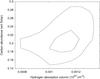 |
Fig. 6 Contour plot of the carbon abundance and the Hydrogen absorption column made using model B. The contours represent the 1 and 2σ confidence regions. |
3.3. G-ratio
 |
Fig. 7 The 2000 and 2002 observation of the OVII He-α triplet. It is clear that the 2002 observation has a higher effective spectral resolution. |
Figure 7 shows the 2000 and 2002 observations of the O vii He-α triplet. This triplet consists of a resonance, forbidden and intercombination line. F (λ = 22.098)1s2s3S1 → 1s2 1S0 is the forbidden transition, I (λ = 21.804, 21.801) is the sum of the two intercombination transitions 1s2p3P1,2 → 1s2 1S0, and R (λ = 21.602) is the resonance transition 1s2p1P1 → 1s2 1S0. Both the 2000 and the 2002 observation are well-fit by three Gaussians with a fixed NH. There are some differences between the two observations, the most notable one being that the F / R ratio is larger in the 2002 observation. In addition, the lines in the 2000 observation are broader, which is an effect of the orientation of the RGS dispersion axis. The total flux in the line triplet is approximately equal between the observations.
An interesting quantity which can be derived from these lines is the so-called G-ratio; G ≡ (F + I) / R (e.g.: Porquet et al. 2010). This quantity equals 0.87 ± 0.09 for 2000 and 1.19 ± 0.09 for 2002, giving a combined ratio of 0.99 ± 0.06. As the 2002 observation has a higher effective resolution, the G-ratio of that observation may be more reliable. Figure 8 shows a plot of G-ratios for different net. The values of the G-ratio for different temperatures reach a constant value as the plasma approaches collisional ionisation equilibrium (CIE). If we take the mean value of the above G-ratios, the calculated G-ratio at high net and kT = 0.2 keV lies just within the error bars and is thus as expected. If the 2002 observation is indeed more reliable, the deduced G-ratio of the plasma lies above this CIE value and the plasma is over-ionised and could be recombining. In principle the excess photons present in the forbidden line should show up as a recombination edge at 16.78 Å. A recombination edge in addition to the already present continuum was not found, however.
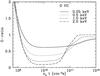 |
Fig. 8 G-ratio of O vii at different temperatures, as a function of ionisation parameter. These curves where calculated using SPEX. |
4. Discussion
We made a detailed spectral analysis of the SNR 0506-68 using mainly the RGS instrument aboard the XMM-Newton telescope. The best fit to the overall mos and RGS spectra is model B: a two component NEI model, of which one component is inverted. We investigated the hypothesis that the plasma is cooling leading to an overionisation, using some known plasma diagnostics. Of those diagnostics, only the 2002 O vii triplet line ratio confirms the hypothesis. There are however, several other physical mechanisms which can cause the observed line ratio.
Resonance scattering can cause photons of resonance lines to be scattered in the direction of least optical depth, reducing the line flux if the optical depth along our line of sight is high. This process was suggested to be responsible for the observed O viiF / R ratio in the SNR DEM L71 (van der Heyden et al. 2003). The scattered photons are not lost, however, so the remnant must have a specific geometry, i.e. it cannot be spherically symmetric, or resonance scattering will have no effect whatsoever. The optical depth in the O vii line equals about 6 in our line of sight, without taking microturbulent velocity into account. The optical depth equals 1, however, at a turbulent velocity of 80 km s-1 and decreases even more at higher values. A high optical depth could result in a significant reduction of the resonance line flux (Kaastra & Mewe 1995), which means that resonance scattering could be significant in this remnant.
Charge exchange occurs when a highly ionised gas enters a neutral gas region, such as a molecular cloud. H-like ions collide with the neutral ions to form excited He-like ions which decay by a radiative cascade. This process enhances the forbidden line due to the higher statistical weight. There have been no reports of neutral gas regions close to the remnant, so the probability of the charge exchange scenario occurring remains uncertain.
4.1. Cooling
As mentioned above, recombination can influence the observed line ratios. For recombination to dominate, the plasma must be over-ionised and thus must have cooled faster than the recombination process happens. We now investigate if SNR 0506-68 can cool fast enough for this to occur.
The expanding plasma cools in two ways: through radiation and due to adiabatic expansion. A timescale for radiative cooling can be obtained by dividing the internal energy of a gas by the luminosity: 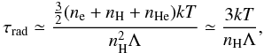 (1)where Λ is the cooling rate in units of erg cm3 s-1, k is Boltzmann’s constant, and nH is the hydrogen/proton number density.
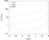 |
Fig. 9 A comparison of the oxygen recombination timescale with the cooling timescale at different densities. Low density favours the appearance of an overionised plasma, because the recombination timescale lowers proportional to the density, as does radiative cooling, but radiative cooling only becomes important at log T ≤ 106 K. These curves where calculated using LMC abundances. It should be noted that a plasma at LMC abundances is less likely to reach an over-ionised state at T < 106 K, because of the lower radiative cooling rate. |
For an adiabatic gas, PVγ = const. By the same token, TVγ − 1 = const. The following formula for the adiabatic cooling timescale can thus be derived for a spherical volume: 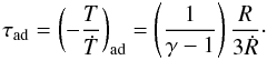 (2)A total cooling timescale as a result of radiative and adiabatic cooling is now given by
  . When a plasma cools, the radiative cooling rate of the remnant is proportional to the density squared. The recombination rate also increases proportional to the density squared. If adiabatic cooling is not important compared to radiative cooling, the remnant will stay in ionisation equilibrium. Radiative cooling is faster than recombination below 106 K or if the elemental abundances are strongly enhanced. For an over-ionised plasma, it is required that τrec > τcool. The recombination timescale for O viii → O vii in the range 106 ≤ T ≤ 107 is approximately equal to (1.3 × 10⁻¹² ne)-1. Using 1, 2 with γ = 5 / 3, this leads to:
 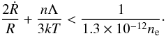 (3)Note that the remnant needs to have reached ionisation equilibrium before adiabatic cooling causes an over-ionised plasma. For R ≃ 10 pc, Ṙ ≃ 400 km s-1, Λ = 3 × 10-23 erg cm3 s-1, corresponding to a 0.2 keV plasma at LMC abundances (Schure et al. 2009) and a density n = 10 cm-3, the recombination timescale (using the above formula) is about five times lower than the cooling timescale, and depends strongly on the density.
To expand the above equation to a larger temperature range, we can rewrite R / Ṙ = β-1t, where β is the expansion parameter and t is the age of the remnant. Values of β vary between about 0.4 for a remnant in the Sedov expansion phase and 0.25 in the snowplough phase. In addition, we can use the temperature dependent O viii → O vii (radiative + dielectronic) recombination rates from Shull & van Steenberg (1982) as well as the complete O radiative cooling curves from Schure et al. (2009).
Figure 9 shows this relation between the cooling and the recombination time using t = 1011 s and β = 0.4. The behaviour at high temperature is dominated by the adiabatic cooling, while radiative cooling becomes important at T < 106 K. An increased density increases the recombination rate, which decreases the likelihood of plasma in SNRs to become over-ionised at temperatures at which radiative cooling is unimportant. It should be noted that the above derivation is a first order estimate. We can however still use it to check if the conditions in SNR 0506-68 are likely to cause an over-ionised plasma. At a T ~ 106 K and n ~ 10 cm-3 the cooling timescale is about two times lower than the recombination timescale. This is a discrepancy with the above calculation, so we can conclude that either our remnant is not in the Sedov stage of evolution (i.e. β < 0.4), or that the shock velocity or density estimations are not right.
We can check if the overionisation observed in other SNRs can be explained using the above relation. In W49B, recombining Fe xxv − xxvi was found. Using their respective recombination and radiative cooling rates at T = 1.5 keV and n = 10 cm-3, the cooling timescale is indeed lower than the recombination timescale.
Note that the above derivation for the cooling rate is somewhat conservative, as we did not take into account dust cooling. This is in particular true for SNR 0506-68, for which Williams et al. (2006) found an infrared luminosity of 8.7 × 1036 erg s-1. This is about 60 times higher than the observed X-ray luminosity. In general dust cooling increases the cooling rate of the plasma, which makes it easier to reach an over-ionised state.
4.2. Explosion parameters
The data obtained from fitting allow us to constrain several interesting parameters. For this we need the volume of the plasma, which we obtained using the Chandra data. The radius of the sphere in which the plasma is contained is about 38′′, which corresponds to a radius of 9.1 pc at a distance of 50 kpc. We therefore estimate the volume of the sphere to be 9 × 1058 cm3. The fact that the radiation is distributed anisotropically over the remnant as well as the fact that the emission does not come from a purely spherical region, can be accounted for by using a filling factor f. A filling factor within 10 − 25% seems reasonable.
Using the normalisation factor nenHVX of the best fit model to the RGS spectra, with ne = nH / 1.2 and VX the volume, we obtain a density nH = 11(f0.1)-0.5 cm-3 and nH = 5(f0.1)-0.5 cm-3 for respectively the cool and the hot component of the non-cooling NEI model, where f0.1 represents a filling factor of 10%. The density of the cool component of the cooling model is slightly higher at 14(f0.1)-0.5. The density of the low T component is somewhat higher than previously found values. Hughes et al. (2006) find densities of 10 − 23 cm-3 using X-ray data, Dickel & Milne (1998) used radio data to find a maximum density of 10 cm-3 and Williams et al. (2006) found a density of 5.8 cm-3 by modelling dust emission in the remnant. These are mean densities over the whole remnant and it is probable that at some locations the densities are higher.
With these densities and the ionisation parameters the shock ages of the cool and hot components are ~ 1200 and ~ 115 yr. Different parts of the remnant were thus shocked at different times, which suggests that there are some density fluctuations in the surrounding ISM, which is also clear from Fig. 1. It has already been hinted by Hughes et al. (2006) that the open cluster HS 114 (Hodge & Sexton 1966), which lies on the brighter, high density side of the remnant, may be the cause of the observed brightness gradient.
The total swept up mass is given by Mswept ~ nHmpfV, where mp is the proton mass.  M⊙ for the cool component and
  M⊙ for the hot component.
Due to the brightness gradient and the fact that a low and high temperature NEI model are necessary to fit the spectrum of the remnant, an age estimation is difficult. Using a Sedov model (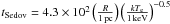 ), the age of the cool component can be estimated at ~ 9000 year, while the age of the hot component equals ~ 4000 year. A Sedov model assumes that the remnant is expanding in a homogeneous medium which, judging from the anisotropic emission, is not quite valid in the case of SNR 0506-68. Since the hot, less dense component of
the plasma is likely to have expanded relatively undisturbed, the age estimation of this component is probably more accurate.
5. Conclusions
-
The SNR 0506-68 is best fit by a two component NEI model, ofwhich one of the components is cooling. This suggests that theSNR may be cooling, but the emission line diagnosticsmarginally agree with this scenario.
-
The most natural explanation for the enhanced G-ratio of the O vii He-α is that part of the plasma is recombining, although resonance scattering cannot be ruled out.
-
When an expanding plasma reaches near-ionisation equilibrium, adiabatic cooling can cause it to become over-ionised.
-
The abundances of SNR 0506-68 are very similar to the mean LMC abundances. This, coupled with the fact that Mswept is fairly high, confirms that the emission is dominated by the emission from the shock heated ISM.
-
Overionisation may be more widespread in mature SNRs than usually thought.
-
The age of the remnant is uncertain and model dependent. However our models and calculations favour the lower age estimate mentioned in the literature, namely ~4000 year.
Acknowledgments
The authors thank the anonymous referee for their positive and useful comments. We would like to acknowledge D. Kosenko and T. van Werkhoven for useful input. S.B. and SRON are supported financially by NWO, The Netherlands Organisation for Scientific Research. The results presented are based on observations obtained with XMM-Newton, an ESA science mission with instruments and contributions directly funded by ESA Member States and the USA (NASA).
References
- Anders, E., & Grevesse, N. 1989, Geochim. Cosmochim. Acta, 53, 197 [Google Scholar]
- den Herder, J. W., Brinkman, A. C., Kahn, S. M., et al. 2001, A&A, 365, L7 [NASA ADS] [CrossRef] [EDP Sciences] [Google Scholar]
- Dickel, J. R., & Milne, D. K. 1998, AJ, 115, 1057 [NASA ADS] [CrossRef] [Google Scholar]
- Gillaspy, J. D., Lin, T., Tedesco, L., et al. 2011, ApJ, 728, 132 [NASA ADS] [CrossRef] [Google Scholar]
- Hayato, A., Bamba, A., Tamagawa, T., & Kawabata, K. 2006, ApJ, 653, 280 [NASA ADS] [CrossRef] [Google Scholar]
- Hodge, P. W., & Sexton, J. A. 1966, AJ, 71, 363 [NASA ADS] [CrossRef] [Google Scholar]
- Hughes, J. P., Hayashi, I., & Koyama, K. 1998, ApJ, 505, 732 [NASA ADS] [CrossRef] [Google Scholar]
- Hughes, J. P., Rafelski, M., Warren, J. S., et al. 2006, ApJ, 645, L117 [NASA ADS] [CrossRef] [Google Scholar]
- Kaastra, J. S., & Mewe, R. 1995, A&A, 302, L13 [Google Scholar]
- Kaastra, J. S., Mewe, R., & Nieuwenhuijzen, H. 1996, in UV and X-ray Spectroscopy of Astrophysical and Laboratory Plasmas, ed. K. Yamashita, & T. Watanabe, 411 [Google Scholar]
- Liedahl, D. A., Kahn, S. M., Osterheld, A. L., & Goldstein, W. H. 1990, ApJ, 350, L37 [NASA ADS] [CrossRef] [Google Scholar]
- Miceli, M., Bocchino, F., Decourchelle, A., Ballet, J., & Reale, F. 2010, A&A, 514, L2 [NASA ADS] [CrossRef] [EDP Sciences] [Google Scholar]
- Ozawa, M., Koyama, K., Yamaguchi, H., Masai, K., & Tamagawa, T. 2009, ApJ, 706, L71 [NASA ADS] [CrossRef] [Google Scholar]
- Porquet, D., Dubau, J., & Grosso, N. 2010, Space Sci. Rev., 157, 103 [NASA ADS] [CrossRef] [Google Scholar]
- Schure, K. M., Kosenko, D., Kaastra, J. S., Keppens, R., & Vink, J. 2009, A&A, 508, 751 [NASA ADS] [CrossRef] [EDP Sciences] [Google Scholar]
- Shull, J. M., & van Steenberg, M. 1982, ApJS, 48, 95 [NASA ADS] [CrossRef] [Google Scholar]
- Smith, R. K., & Hughes, J. P. 2010, ApJ, 718, 583 [NASA ADS] [CrossRef] [Google Scholar]
- Smith, R. K., Brickhouse, N. S., Liedahl, D. A., & Raymond, J. C. 2001, ApJ, 556, L91 [NASA ADS] [CrossRef] [Google Scholar]
- Someya, K., Bamba, A., & Ishida, M. 2010, PASJ, 62, 1301 [NASA ADS] [Google Scholar]
- Turner, M. J. L., Abbey, A., Arnaud, M., et al. 2001, A&A, 365, L27 [NASA ADS] [CrossRef] [EDP Sciences] [Google Scholar]
- Uchida, H., Tsunemi, H., Katsuda, S., Kimura, M., & Kosugi, H. 2009, PASJ, 61, 301 [NASA ADS] [Google Scholar]
- van der Heyden, K. J., Bleeker, J. A. M., Kaastra, J. S., & Vink, J. 2003, A&A, 406, 141 [NASA ADS] [CrossRef] [EDP Sciences] [Google Scholar]
- Williams, B. J., Borkowski, K. J., Reynolds, S. P., et al. 2006, ApJ, 652, L33 [NASA ADS] [CrossRef] [Google Scholar]
- Yamaguchi, H., Ozawa, M., Koyama, K., et al. 2009, ApJ, 705, L6 [NASA ADS] [CrossRef] [Google Scholar]
All Tables
Line fluxes of a number of emission lines calculated with and without hydrogen absorption.
All Figures
|
Fig. 1 A smoothed Chandra RGB image of the SNR 0506-68. The arrows denote the direction of the RGS dispersion directions. The RGS field of view covers the remnant completely. Red corresponds to O vii (0.53−0.61 keV), green to Fe l (0.79 − 0.89 keV) and blue to Mg xi (1.25 − 1.41 keV). The arrows denote the dispersion axis orientation of the 2000 (upper arrow) and the 2002 (lower arrow) observations. |
| In the text | |
|
Fig. 2 The total 2001 RGS1 and RGS2 spectrum of SNR 0506-68 in the range 5 − 35 Å. The best fit two-component NEI model (see text) is plotted in red. |
| In the text | |
|
Fig. 3 Plot of the MOS 1 and MOS 2 data of 2002. The model seems to fit the data well. |
| In the text | |
|
Fig. 4 A plot of the mos 2 data with model A and model B in the range 0.8 − 1.8 keV. The bottom part of the figure shows the relative error between model A and the data, while the dashed red line shows model B – model A. It is clear that model B follows the overall shape of the data better than model A. For example, model A shows a residual at ~1.25 keV, whereas model B improves the fit of this region due to the Fe xvii recombination edge at 1.26 keV. |
| In the text | |
|
Fig. 5 The 2002 RGS1 and RGS2 spectrum of SNR 0506-68 in the range 14−18 Å. The best fit two-component NEI model (see text) is plotted in solid black. The model has trouble fitting the 15 and 17 Å Fe xvii as well as the O viii Ly β/Ly α line ratio. |
| In the text | |
|
Fig. 6 Contour plot of the carbon abundance and the Hydrogen absorption column made using model B. The contours represent the 1 and 2σ confidence regions. |
| In the text | |
|
Fig. 7 The 2000 and 2002 observation of the OVII He-α triplet. It is clear that the 2002 observation has a higher effective spectral resolution. |
| In the text | |
|
Fig. 8 G-ratio of O vii at different temperatures, as a function of ionisation parameter. These curves where calculated using SPEX. |
| In the text | |
|
Fig. 9 A comparison of the oxygen recombination timescale with the cooling timescale at different densities. Low density favours the appearance of an overionised plasma, because the recombination timescale lowers proportional to the density, as does radiative cooling, but radiative cooling only becomes important at log T ≤ 106 K. These curves where calculated using LMC abundances. It should be noted that a plasma at LMC abundances is less likely to reach an over-ionised state at T < 106 K, because of the lower radiative cooling rate. |
| In the text | |
Current usage metrics show cumulative count of Article Views (full-text article views including HTML views, PDF and ePub downloads, according to the available data) and Abstracts Views on Vision4Press platform.
Data correspond to usage on the plateform after 2015. The current usage metrics is available 48-96 hours after online publication and is updated daily on week days.
Initial download of the metrics may take a while.